Microbiology (2003), 149, 2859–2871
DOI 10.1099/mic.0.26211-0
A three-dimensional, stochastic simulation of biofilm growth and transport-related factors that affect structure Ivan Chang,1 Eric S. Gilbert,2 Natalya Eliashberg1 and Jay D. Keasling1 1
Department of Chemical Engineering, University of California, Berkeley, CA 94720-1462, USA
Correspondence Jay D. Keasling
[email protected]
Received 23 December 2002 Revised
25 June 2003
Accepted 26 June 2003
2
Department of Biology, Georgia State University, Atlanta, GA 30303, USA
Biofilm structural heterogeneity affects a broad range of microbially catalysed processes. Solute transport limitation and autoinhibitor production, two factors that contribute to heterogeneous biofilm development, were investigated using BacMIST, a computer simulation model. BacMIST combines a cellular automaton algorithm for biofilm growth with Brownian diffusion for solute transport. The simulation represented the growth of microbial unit cells in a three-dimensional domain modelled after a repeating section of a constant depth film fermenter. The simulation was implemented to analyse the effects of various levels of transport limitation on a growing single-species biofilm. In a system with rapid solute diffusion, cells throughout the biofilm grew at their maximum rate, and no solute gradient was formed over the biofilm thickness. In increasingly transport-limited systems, the rapidly growing fraction of the biofilm population decreased, and was found exclusively at the biofilm–liquid interface. Trans-biofilm growth substrate gradients also deepened with increasing transport limitation. Autoinhibitory biofilm growth was simulated for various rates of microbially produced inhibitor transport. Inhibitor transport rates affected both the biofilm population dynamics and the resulting biofilm structures. The formation of networks of void spaces in slow-growing regions of the biofilm and the development of columns in the fast-growing regions suggested a possible mechanism for the microscopically observed evolution of channels in biofilms.
INTRODUCTION Microbial biofilms are communities of bacteria that attach to surfaces and form heterogeneous three-dimensional structures (Stickler, 1999). The functional significance of biofilm structural heterogeneity extends to diverse areas of applied microbiology. In the clinical setting, mature biofilm structure contributes to antibiotic resistance through a variety of mechanisms (Mah & O’Toole, 2001). In the industrial setting, heterogeneous biofilm and aggregate structure affects denitrification processes (de Beer & Schramm, 1999; Schramm et al., 1999), and modelling results indicate that heterogeneous biofilm formation influences the onset of metal corrosion (Picioreanu & van Loosdrecht, 2002). In general, biofilm architecture affects mass transfer in biofilms (Rasmussen & Lewandowski, 1998; Stoodley et al., 1999), and is relevant when considering microbial biofilms as catalysts as well as for managing the efficacy of biocides and compounds that influence biofilm development, e.g. furanones (Ren et al., 2001, 2002). Abbreviations: CA, cellular automata; CDFF, constant depth film fermenter.
0002-6211 G 2003 SGM
Printed in Great Britain
An approach that has provided new insight into the factors that influence biofilm structure has been the use of cellular automata (CA) simulations. CA simulations of biofilms represent cells as discrete units that replicate stochastically in a two- or three-dimensional domain according to a set of rules, and they are effective at simulating the heterogeneity in biofilms (Pizarro et al., 2001). A general feature of CA models of biofilms is their ability to dynamically generate a range of observed biofilm morphologies using a minimal set of assumptions about cell behaviour; however, computational time constraints have limited most models to two dimensions (Hermanowicz, 1999, 2001; Pizarro et al., 2001). An approach to improving computational efficiency has been to decouple solute transport from stochastic bacterial growth by the use of numerically solved, partial differential equations to describe substrate diffusion (Picioreanu et al., 1998). This method allows the CA model to extend to three dimensions more easily, but does so at the expense of losing heterogeneity in the solute concentration profile. Another new trend in CA biofilm models is an individual-based modelling approach, which allows for variability in each of the cells in the simulation (Kreft et al., 2001). Overall, CA models have been employed 2859
I. Chang and others
to simulate several diverse microbial biofilm systems, including a single-species nitrifying biofilm (Picioreanu et al., 1998), a dual-species nitrifying biofilm (Kreft et al., 2001), and an anaerobic biofilm comprising a sulfate reducer and a methanogen (Noguera et al., 1999). In this work, an individual-based three-dimensional CA model, coupled with discrete Brownian diffusion, was developed. The model, BacMIST (Multi-threaded Independent Solute Transport), uses several techniques to allow for a tractable stochastic solute diffusion simulation in three dimensions in order to retain the effects of local solute concentration heterogeneity. BacMIST simulated two factors that could contribute to the structural heterogeneity in the biofilm. In one scenario, solute transport limitations into the biofilm were considered. Transport limitations affect biofilm structure in various ways, depending on the ecology of the system under consideration. For example, limited oxygen diffusion altered the composition and distribution of microbial populations in nitrifying biofilm-like communities (Vogelsang et al., 2002). Similarly, transport of substrate into membrane-aerated biofilm reactors influenced the size, location and number of active zones within the biofilm (Casey et al., 1999). On the other hand, the population size of sulfate-reducing bacteria near the substratum of a wastewater biofilm remained stable over time as a result of substrate transport limitations (Ito et al., 2002). In a second scenario, the influence of microbially generated autoinhibitor compounds was evaluated. Autoinhibition may result from the microbial synthesis of metabolic end products that produce unfavourable changes in the organism’s environment, such as the lowering of pH upon production of excessive acetate by Escherichia coli growing on glucose (Ingraham & Marr, 1996). Alternatively, the end product itself may also act as an inhibitor, as in the production of methanol by a Pseudomonas sp. growing on methane (Wilkinson et al., 1974). Autoinhibitory compounds are found in several species of surface-colonizing marine bacteria that contribute to biofouling, and have been postulated to function in maintaining bacterial community diversity (Holmstroem et al., 2002). More generally, bacterial programmed cell death, catalysed by autolysins, contributes to developmental processes in a range of diverse bacteria (Lewis, 2000), and may affect biofilm development. The CA model described here accounts for transport of substrate and inhibitors as well as cell death and examines their impact on biofilm structure.
MODEL DESCRIPTION Reactor geometry. A useful experimental system in which to
model biofilm growth and development is the constant depth film fermenter (CDFF). This biofilm reactor was first introduced in 1974, and since then has been improved and developed by Wimpenny and colleagues, who provide a detailed description of the system (Wimpenny et al., 1993). The CDFF approximates a steady state by only allowing biofilm growth in recessed regions of constant depth cut into the surface of a solid plate. A scraper bar constantly passes 2860
over the plate surface, removing any biofilm that grows above the tops of the recesses. Fresh growth medium is continuously fed in and distributed over the CDFF surface, aided by the spreading action of the scraper bar, and spent medium is drained out of the apparatus through an outlet port. Since the biofilm is grown in the protected recessed regions, it is not subjected to hydrodynamic forces that can potentially contribute to biofilm detachment and channel formation. This protected geometry also implies that transport processes in the biofilm growth regions of the CDFF are dominated by diffusion. Simulation domain. Growth simulations performed using BacMIST
take place in a three-dimensional spatial domain representing a section of a CDFF recessed region. The domain is discretized into sites on a cubic lattice, and each site or unit cell in the lattice was assumed to be 1 mm3. The domain organization used in this work shares similarities with the CA simulation presented by Hermanowicz (1999), except the domain in this work is in three dimensions. Each of the sites is occupied by either a unit volume of biomass (which could be one or more bacterial cells, possibly embedded in extracellular polymeric substances) or an equivalent volume of liquid. The domain is bounded on one side by a solid surface, the substratum, on which the biofilm grows. The opposite side of the domain represents the top of the recessed region in the CDFF, the ‘shear boundary’. Any cells reaching this point of the domain will be ‘scraped’ from the biofilm and removed from the simulation as they are swept away by passing liquid. In the other two directions, parallel to the growth surface, periodic boundary conditions are implemented. Any cell pushed out of the domain through a periodic boundary will be replaced by an identical cell entering the domain in the same place at the opposite boundary. In this way, the simulation domain represents a repeating unit of an infinite biofilm of finite thickness. For the simulation tests involving structural observation, special care is needed to choose a domain size that would not create an overlapping, aliasing effect. It was empirically determined from numerous trials that a domain size having width and length dimensions greater than height usually gives a more lucid three-dimensional plot, while a cubic domain results in clearer two-dimensional slice images. Simulated activities. A natural biofilm begins as a small population of cells that have individually adhered to a solid substratum. As these cells grow and divide, their offspring spread over the surface and eventually form an adherent, multicellular contiguous population. Analogously, the biofilm growth simulation begins with a randomly placed population of substratum ‘colonizers’. A file with the descriptions and initial locations of the colonizers must be processed by the simulation before the biofilm growth phase can begin. One colonizing cell is sufficient to initiate a biofilm.
Once the substratum is colonized, the biofilm growth simulation cycles through four classes of behaviours during each time step. (i) Solutes are transported by random-walk diffusion, updating their locations throughout the simulation domain. (ii) Cells consume and produce solutes based on food and inhibitor solute concentrations in their immediate vicinities. As a result, cell growth counters are updated, as are overall solute numbers. (iii) Cells that have consumed enough growth substrate divide. Randomly chosen cells in the population die and lyse. Cells that have moved beyond the shear boundary are also removed from the simulated biofilm. Thus, cell numbers and locations are updated. (iv) The thin interface layer representing the diffusion boundary layer is replenished with solutes to cover the solutes lost in consumption. These behaviours are described in more detail in the following sections. A flow diagram describing the basic simulation is provided in Fig. 1. Solute transport. Diffusion can be modelled stochastically by a large
number of particles undergoing random walks in space. Each random walk consists of a series of equal-length, straight-line movements Microbiology 149
Stochastic simulation of biofilms
Fig. 1. Flow diagram for basic simulation. Shaded boxes indicate stochastic processes. Shadowed boxes indicate complex events described by flow diagrams in Fig. 2.
interspersed with an equal number of completely random direction changes. This walk simulates the motions exhibited by molecules or small particles which translate due to system internal energy, and which change direction due to collisions with other particles in the same system. While any one particle can be moving in any given direction at a specific time, the net motion of the population of particles will be down the particle concentration gradient. Each cell in the biofilm growth simulation is a consumer, and possibly a producer, of various solutes. As the biofilm grows and cells are shifted around due to division, the boundary conditions for the solute diffusion problem continuously change. Essentially, the problem is reduced to solute diffusion in three dimensions among a large number of moving sources and sinks. When there are multiple cell types, with different consumption and production patterns, such a problem is extremely complex if implemented using the Fickian description of diffusion. For this reason, random-walk diffusion was chosen as the paradigm for solute transport in the biofilm simulation. Some simplifications were made in the implementation of randomwalk diffusion as the transport mechanism in the biofilm simulation. Instead of describing individual solute molecules, particles represent ‘quanta’ of solute. Each quantum contains some number of solute molecules, so that a relatively small number of quanta of a solute in a simulation lattice cube can represent a moderately high concentration of that solute. Solute diffusivity of a lattice cube not occupied by a biofilm cell is set higher than the diffusivity of a cube containing a http://mic.sgmjournals.org
biofilm cell. Although data may be lacking in the case of bacterial colonies, diffusion of solutes through tissue and gels has been measured by a number of groups (Berk et al., 1996; Johnson et al., 1996) and is, in general, orders of magnitude lower than diffusion in free solution. An effective diffusivity D can be defined in a threedimensional system (Lee et al., 1989): D~
na2 6Dt
ð1Þ
where n is the number of steps taken in the random walk, a is the length of a single step, and Dt is the time interval over which the n steps take place (the units of the parameters used in the equations are given in Table 1). A flow diagram describing the implementation of solute transport is provided in Fig. 2(a). Microbial consumption and production of solutes. Following
a round of Brownian diffusion, each successful solute particle in the simulation is located somewhere in the active solute domain, and each of these locations is in the interior of a lattice cube of the domain grid. In order for a solute particle to be transferred from the diffusion boundary layer to the biofilm, there must be a concentration gradient for the diffusion. Otherwise, the solute will stay in the boundary layer or diffuse out of the biofilm active domain if the concentration of solute inside the biofilm becomes equal to or greater than the bulk. If a solute quantum is in a grid space occupied by a cell, that cell has an opportunity to act on or be influenced by that solute, depending on the relationship between them. During 2861
I. Chang and others
Table 1. Parameters and their units Parameter n a Dt
YS/C Pc td m
Cbulk kr,i i Ithresh Factor kd Lf XC S* x*
Definition
Units
Number of simulation steps Length of diffusion step Time interval Inverse yield coefficient Single-cell, single-substrate consumption probability Doubling time Specific growth rate Bulk concentration of substrate Specific substrate consumption rate constant Number of inhibitors per grid space Threshold number of cell-specific inhibitors Extent of additional inhibition from each inhibitor quantum over threshold Death rate constant Maximum biofilm depth Maximum biofilm density Non-dimensionalized form of substrate concentration Non-dimensionalized form of biofilm depth
the consumption and production phase of the growth simulation, a cell examines all the solutes in its grid space, and acts or does not act on each. If the cell encounters a quantum of its growth substrate, it may be consumed. Simulated cell consumption of growth substrate is a process first order in cells and first order in substrate. A single cell consuming a single substrate, therefore, does so with probability Pc=kr,iDt in a single time step Dt, where kr,i is the second-order consumption rate constant. A cell consuming a substrate is eligible to synthesize one or more quanta of product, if solute production is one of its activities. Product quanta are produced, upon substrate consumption, with a probability dependent on the stoichiometric or yield ratio of product to solute for that particular cell species. A flow diagram describing the implementation of solute consumption by a single cell is provided in Fig. 2(b). Consumption- and growth-related parameters provided to a given simulation include the simulation time step, Dt, the single cell–single substrate consumption probability, Pc, and the inverse yield constant, YS/C, quantifying how many substrate quanta must be consumed for a cell to divide in two. If C, the mean concentration (number of quanta per grid space) of growth substrate available to a cell, is also known, an expected cell doubling time, td, can be calculated as follows: td ~
(YS=C )(Dt) (Pc )(C)
ð2Þ
From the doubling time, the mean growth rate, m, can be calculated: k~
ln2 td
ð3Þ
If a growth substrate from the liquid bulk is available to a cell, a maximum growth rate, mmax, is calculated, assuming that the greatest substrate concentration available will be, on average, the bulk concentration, Cbulk. kmax ~
(ln 2)(Pc )(Cbulk ) (YS=C )(Dt)
ð4Þ
The growth of a cell can be affected by the proximity of inhibitor 2862
mm min quanta per cell mm3 per cell min min21 quanta mm23 mm3 per cell min21 quanta quanta
min21 mm Cells mm23
solutes. An inhibitor in the simulation acts by decreasing the probability that a cell will consume its growth substrates. In the presence of inhibitor, the specific consumption rate constant, kr,i is multiplied by an inhibition factor, calculated as follows: ( Factor{(i{I thresh ) if i>Ithresh multiplier~ ð5Þ 1 if i