VIVECHAN International Journal of Research, Vol. 7, Issue 1, 2016
ISSN No. 0976-8211
A Three Phase Transformer Modelling For Distribution System *
Debojyoti Sen , Aditi Dixit and Anshul Tiwari Department of Electrical and Electronics IMS Engineering College, Ghaziabad, India. *
[email protected] Abstract The purpose of this paper to present that how a three phase transformer can be modelled in some definite parameters that can be used to represent a transformer in distribution system .These model will follow Kirchhoff's current, voltage law & the ideal relationship between primary & secondary side of transformer. This paper is limited to modelling of Delta-Grounded Wye connection. Keywords-Power system, Three phase transformer, Transformer models
Introduction A transformer is a machine that is used to change the level of voltage of a system without changing frequency. It is necessary to convert high level voltage to low level voltage for proper operation of equipment. Three phase transformers are used in distribution system for changing the transmission level voltage to distribution level voltage (Kersting, 1999) (Philips & Kersting, 1987). It is impossible to designing any system without transformer. Transformer is mostly used in every part of power system. So for designing a power system or for analysis purpose it is necessary that the whole system model should be modelled correctly (Philips & Kersting, 1990; Kumar & Selvan, 2008). These models or parameters can also be used for computer calculation. H1-A
H2-B
IA
H3-C
IB
IC
I AC
I BA
I CB
Ia
Ib
Ic
I
nt
Zt a
X1-a
Zt b
Vag
+ X2-a
IE
Zt c
Vag
V + ag X3-c g -
Figure 1: 1 Delta-Grounded Wye Connection nt =
VLLRated High Side VLNRated Low Side 79
VIVECHAN International Journal of Research, Vol. 7, Issue 1, 2016
ISSN No. 0976-8211
The ideal secondary side voltages is given by: VAB VBC VCA
0 0 -nt
=
-nt
U Vta -nt * Vtb Vtc 0
0 0
(1)
[VLLABC ] = [AV]*[Vtabc ]
Where -nt
0 0 -nt
[AV] =
0 0
0 -nt 0
Here the primary line-to-line voltages at Node n as functions of the ideal secondary voltages has been determined (Kersting, 1993). However, required relationship is between equivalent line-to-neutral voltages at Node n and the ideal secondary voltages (Anderson, 2008; Grainger & Willaim, 1994). Hence line-to-neutral voltages at node n from line-to-line voltages are determined by theory of symmetrical components. The known line-to-line voltages are transformed to their sequence voltages by: [VLL012 ] =[A 3] - 1 * [VLLABC ] [A5] -1 =
1 12 1 a5 1 a5
(2)
1 a3 a3 2
as=1.0/120 VLN0 VLN1 VLN2
=
1 0 0
0 t3* 0
0 VLL0 0 * VLL1 t3 VLL2
(3)
[VLN 012 ] = [T] * [VLL012 ]
Where ts =
1 3
/30
The equivalent line-to-neutral voltages as functions of the sequence line- to-neutral voltages are: (4)
[VLNABC ]=[A3]* [VLN 012 ]
Substitute Equation 3 into Equation 4 [VLNABC ] = [A3]*[T]* [VLL012 ]
(5)
Substitute Equation 2 into Equation 5 [VLNABC ] = [W]* [VLLABC ]
Where
[W] = [A3]*[T]*[A3]- 1
2 1 = * 0 2 3 1 0 1
0 1 2
(6)
Equation 1 can now be substituted into Equation 6: [VLN ABC ] = [W]* [AV]*[ Vt abc ] = [at ]*[Vt abc ]
(7)
Where at =
- nt 3
0 2 1 0 2 1
1 2 0
Copyright 2016 IMSEC
80
D Sen et al.: A Three Phase Transformer Modelling For Distribution System
The ideal secondary voltages as functions of the secondary line-to-ground voltages and the secondary line currents are: [Vt abc ] = [VLG abc ] + [Ztabc ]*[Iabc ]
Here is no such restriction that the impedances of the three transformers be equal. Substitute Equation 8 into Equation 7:
(8)
[VLN ABC ] = [a t ]*[[VLGabc ] + [Ztabc ]*[Iabc ]
[VLN ABC ] = [a t ]*[VLGabc ] + [b t ]*[Iabc ]
Where bt = [at ]*[Ztabc ] =
- nt 3
*
0 Zta 2.Zta
2. Ztb 0 Zt b
(9) Ztc 2.Ztc 0
The line currents can be determined as functions of the delta currents by applying Kirchhoff's current law: IA 1 IB = 0 IC -1
IAC 0 - 1 * IBA ICB 1
-1 1 0
[I ABC ] = [D ]*[IDABC ]
(10)
The matrix equation relating the delta primary currents to the secondary line currents is given by: IAC IBA = ICB
1 * 0 nt 0 1
0 0 Ia 1 0 * Ib 0 1 Ic
[IDABC ] = [AI]*[Iabc ]
(11)
Substitute Equation 11 into Equation 10: [I ABC ] = [D ]*[AI]*[Iabc ] = [ct ]*[VLG abc ] + [dt ]*[Iabc ] [I ABC ]= [dt ]*[I abc ]
Where
1 - 1 0 1 d t = [ D]*[AI] = . 0 1 - 1 nt - 1 0 1 ct = 0
The derivation of the generalized matrices [A] and [B] begins with solving Equation (1) for the ideal secondary voltages: [Vtabc ] = [AV]- 1 * [VLLABC ]
(12)
Bu s Zeq
Zeq
Load
The line-to-line voltages as functions of the equivalent line-to-neutral voltages are [VLLABC ] = [D]* [VLNABC ]
Where
(13)
1 - 1 0 [D] = 0 1 - 1 - 1 0 1
81
VIVECHAN International Journal of Research, Vol. 7, Issue 1, 2016
ISSN No. 0976-8211
Substitute Equation 13 into Equation 12 [Vt abc ] = [AV] - 1*[D]* [VLNABC ] = [A t ]* [VLNABC ]
(14)
Where
1 0 - 1 1 A t = [AV] - 1 *[D] = . - 1 1 0 nt 0 - 1 1
Substitute Equation 8 into Equation 12 [VLG abc ] + [Ztabc ]*[I abc ] = [A t ]* [VLNABC ]
[VLG abc ] = [At ]* [VLN ABC ] -[Bt ]*[Iabc ]
Where Bt = [Zt abc ] =
Zta 0 0
0 Ztb 0
0 0 Zt c
Ct = 0 1 - 1 0 1 D t = [ D ]*[AI] = . 0 1 - 1 nt - 1 0 1
Power Flow Studies Power flow studies of an interconnected means to analysing the power flow in various segments of power system. Power Flow studies emphasizes on the different aspects of AC power like real power, reactive power, voltages & voltage angles (Grainger & William, 1994; Philips & Kersting, 1990). This analysis is done in steady state condition. Power flow is necessary for future planning & to find the optimal operation of existing system (Sedghi, 2012; Gupta, 2013). The basic information we get from the power flow studies is value of voltage magnitude & voltage angle at different buses of power system (Ranjan & Das, 2003). Power flow studies can be utilised to determine following: 1. Voltage magnitudes and angles at all nodes. 2. Line flow in each line section specified in KW and KVAR, amps and degrees, or amps and power factor. 3. Total input KW and KVAR. 4. Power loss in each line section.
Total feeder power losses.
Load KW and KVAR based upon the specified model for the load.
Results Input values:T/F Rating Sa=750KVA 2000KVA .85lag 12.47-2.4KV Z=.01+.06j Copyright 2016 IMSEC
Loading
Sb=1000KVA .9lag Sc =1250KVA .95lag
82
D Sen et al.: A Three Phase Transformer Modelling For Distribution System
Tolerance=.006pu Specified Voltage at bus1=12470 V (30,-90,150) Assumed voltage at last bus= 2400 V (-30,-150, 90) Phase impedance=1+6j% Conclusions
AT BU S
Bus 1
Bus 2
Bus 3
Bus 4
Specifications
Phase A
Phase B
Phase C
Voltage magnitude(KV)
7.199
7.199
7.199
Voltage phase angle
0
-120
120
Current magnitude(amp)
128.302
166.14
156.218
Current phase angle
-25.78
-143.24
83.53
Voltage magnitude(KV)
7.168
7.171
7.165
Voltage phase angle
-0.1429
-120.23
119.820
Current magnitude(amp)
128.302
166.14
156.218
Current phase angle
-25.78
-143.24
83.53
Voltage magnitude(KV)
2.349
2.342
2.334
Voltage phase angle
-31.18
-151.70
87.77
Current magnitude(amp)
329.32
454.0334
563.98
Current phase angle
-63.63
-179.35
65.077
Voltage magnitude(KV)
2.2781
2.2001
2.2128
Voltage phase angle
-31.83
-153.52
83.10
Current magnitude(amp)
329.32
454.03
563.98
Current phase angle
-63.63
-179.35
65.077
83
VIVECHAN International Journal of Research, Vol. 7, Issue 1, 2016
ISSN No. 0976-8211
This paper presents the modelling of delta-grounded wye transformer with the help of determination of a,b,c and d parameters and then these modeled transformers can be used to perform the power flow studies in much bigger and complex power systems .With the help of power flow studies we can determine the power losses in each line and total feeder power losses. So, the modelling of transformer simplifies the calculation in power flow studies and helps in quick determination of losses. References Grainger, J. J., and William D. S. (1994) Power system analysis. McGraw-Hill. Gupta, J. B. (2009) Fundamentals of Electrical Engg. & Electronics, SK Kataria and Sons. Hill, E. F., William, D., Stevenson, Jr. (1968) An improved method of determining incremental loss factors from power system admittances and voltages, Power Apparatus and Systems, IEEE Transactions, 6, 1419-1425. Kersting, W. H. (1993) Distribution feeder analysis, Distribution system modelling and analysis, pp. 323334. Kersting, W. H. and Phillips, W. H. (1987) A radial three-phase power flow program for the personal computer, Proc. Frontiers of Power Conf. Kersting, W. H. and Phillips, W. H. (1990) Distribution system short circuit analysis, Energy Conversion Engineering Conference, 1990.IECEC-90.Proceedings of the 25th Intersociety.Vol.1, IEEE. Kersting, W. H., Phillips, W. H. and Wayne C. (1999) A new approach to modeling three-phase transformer connections, Industry Applications, IEEE Transactions, 35(1), 169-175. Kumar, K. V., and Selvan, M. P. (2008) A simplified approach for load flow analysis of radial distribution network with embedded generation, TENCON 2008-2008 IEEE Region 10 Conference, IEEE. Kundur, P. et al. (2004) Definition and classification of power system stability IEEE/CIGRE joint task force on stability terms and definitions, Power Systems, IEEE Transactions on 19(3), 1387-1401. Ranjan, R., and D.A.S. (2003) Simple and efficient computer algorithm to solve radial distribution networks, Electric power components and systems, 31(1), 95-107. Sedghi, M. and Aliakbar-Golkar, M. (2012) Analysis and Comparison of Load Flow Methods for Distribution Networks Considering Distributed Generation, International Journal of Smart Electrical Engineering 1.1.
Copyright 2016 IMSEC
84