HAN ET AL.: A TIMING-BASED SCHEME FOR ROGUE AP DETECTION
1
A Timing-Based Scheme for Rogue AP Detection Hao Han, Bo Sheng, Student Member, IEEE, Chiu C. Tan, Student Member, IEEE, Qun Li, Member, IEEE, and Sanglu Lu, Member, IEEE Abstract—This paper considers a category of rogue access points (APs) that pretend to be legitimate APs to lure users to connect to them. We propose a practical timing-based technique that allows the user to avoid connecting to rogue APs. Our detection scheme is a client-centric approach that employs the round trip time between the user and the DNS server to independently determine whether an AP is a rogue AP without assistance from the WLAN operator. We implemented our detection technique on commercially available wireless cards to evaluate their performance. Extensive experiments have demonstrated the accuracy, effectiveness and robustness of our approach. The algorithm achieves close to 100% accuracy in distinguishing rogue APs from legitimate APs in lightly-loaded traffic conditions, and larger than 60% accuracy in heavy traffic conditions. At the same time, the detection only requires less than one second for lightly-loaded traffic conditions and tens of seconds for heavy traffic conditions. Index Terms—Wireless LAN, IEEE 802.11, rogue access point, round trip time.
✦
1
I NTRODUCTION
T
HE
proliferation of IEEE 802.11 networks (WLAN) in public spaces such as airports and coffee houses has increased the interest of security and privacy when using such networks. A thread called rogue access points, or rogue APs, has emerged as an important security problem in WLANs [1], [2], [3], [4], [5], [6], [7]. A rogue AP is defined as an illegal access point that is not deployed by the WLAN administrator. Two types of rogue APs can be set with different equipments. The first type uses a typical wireless router connected directly into an Ethernet jack on a wall. The second type of rogue APs are set on a portable laptop with two wireless cards, one connected to a real AP and the other configured as an AP to provide Internet access to WLAN stations. We will further explore the differences between these two types of rogue APs in later sections. In this paper, we focus on the detection of the second type of rogue APs. Fig. 1 illustrates that a laptop with two wireless adaptors can be easily set as the rogue AP considered in this paper. For example, we let the internal wireless adaptor connect to a legitimate AP, and external wireless adaptor pretend to be a real AP to induce users. In Linux, running command iptables -t nat -A POSTROUTING -o interface -j MASQUERADE can bridge packets from one adaptor to the other easily. According to 802.11 standard, when multiple APs exist nearby, a WLAN client will always choose the AP with the strongest signal to associate. To attract clients, therefore, a rogue AP • H. Han, B. Sheng, C. Tan and Q. Li are with the Department of Computer Science, College of William and Mary, VA, 23187. E-mail: {hhan, shengbo, cct, liqun}@cs.wm.edu • H. Han and S. Lu are with the State Key Laboratory for Novel Software Technology, Nanjing University, China. E-mail:
[email protected]
Fig. 1: Demonstration of the hardware for setting up a rogue AP. The requirement is only a laptop with two wireless adaptors: A is an internal wireless adaptor which is connected to a legitimate AP, and B is an external wireless adaptor which behaves as a legitimate AP to induce users.
needs to be close to clients so that its signal can be stronger than other legitimate APs. The rogue AP can then passively wait for users to connect to it, or actively send a fake de-associate frame to force users to change connection. Note that, the setting here only demonstrates the basic steps of setting up a rogue AP to launch attacks. In practice, a rogue AP needs further configuration to avoid easy detections, such as spoofing MAC address, SSID and vendor name, setting up a DHCP server to assign valid IP addresses to connected clients. Once an innocent client is connected to a rogue AP, the adversary can manipulate and monitor the incoming and outgoing traffic of the client, and further launch different kinds of attacks. For instance, the adversary can easily launch phishing attacks by redirecting the user’s web page request to a fake one to steal the user’s sensitive information such as bank account and password. The previous work has explored several approaches for rogue AP detection. One category of solutions is to measure some identities/fingerprints of an AP such as
HAN ET AL.: A TIMING-BASED SCHEME FOR ROGUE AP DETECTION
SSID, MAC address, RSSI, and clock skew. A rogue AP is detected when its identities are compared to those of legitimate APs. The other category of approaches is to analyze network traffic at the gateway to detect the presence of rogue APs (more details are described in section 2). These existing approaches cannot effectively detect rogue APs from the client’s side, especially in the strong adversary model considered in this paper, where “smart” rogue APs are aware of the current detection schemes, and have opportunities to circumvent the detections. Here we list some challenges for designing a detection scheme: • Clients may not have access to the information about legitimate APs, especially those APs deployed in hotspots. Therefore, it is not possible to compare the identity of an AP with that of authorized APs stored in the database. • Clients have less privileges than administrators. They are limited by the settings of the network. For example, clients cannot set dedicated servers for detection. They cannot use the existing protocols that are not supported by the local network. Also, without the assistance from network administrators, it is not easy for clients to collect network traffic at the gateway. Therefore, the second category of the previous approaches is not possible. • Smart rogue APs know the detection schemes and manage to escape from detections. They can forge their identities, block or fake certain unimportant messages, and directly reply to clients without forwarding messages to legitimate APs. Therefore, simple defenses could be easily circumvented. In Section 3.2, we will look at the strategy for a sophisticated adversary in more detail. In this paper, we propose a timing-based rogue AP detection technique that allows the user to independently determine whether an AP is legitimate or not without assistance from the WLAN operator. To the best of our knowledge, we are the first to propose a rogue AP detection scheme that can be implemented purely by end users. Our main contributions are listed as follows: (1) We extend the work in [8] by using an outlier filtering algorithm to reduce false detection, and dynamically adjusting the number of samples in each test to reduce the detection time without sacrificing accuracy. Furthermore, we improve our evaluation to include more complex scenarios. (2) We propose a timing-based rogue AP detection algorithm that is compatible with the existing networking protocols, and can be applied to 802.11 network (including both 802.11b and 802.11g) without further modifications by network administrators. (3) Our solution can detect powerful rogue APs that actively try to avoid detections as opposed to an “accidental” rogue AP deployed, for example, by an innocent employee in an office [9]. (4) We implement our scheme using commercial offthe-shelf wireless cards and evaluate the performance
2
through real experiments at two campus WLANs. Results from extensive experiments show our algorithm achieves almost 100% accuracy in distinguishing rogue APs from legitimate APs in lightly-loaded traffic conditions, and more than 60% accuracy in heavy traffic conditions. The rest of the paper is organized as follows. Sections 2 and 3 discuss the related work, and problem formulation respectively. Our algorithm is detailed in Section 4, and our implementation is presented in Section 5. We depict the evaluation results in Section 6 and conclude in Section 7.
2
R ELATED WORK
The threat of rogue APs has attracted significant attentions from both industrial and academic researchers. We can classify rogue AP detection into two categories. The first category relies on wireless sniffers to monitor wireless network to detect rogue APs. These sniffers usually scan the spectrum at 2.4 and 5GHz for unauthorized traffic. The sniffers will alert the system administrators when such traffic is detected. Some commercial products [1], [2], [3] have been developed using this technique. In these products, a variety of identifying characteristics including MAC addresses, vendor name, and SSID are used to distinguish between a legitimate AP and a rogue AP. Other alternatives include collecting RSS values [10], radio frequency variations [11], and clock skews [12] as fingerprints to identify rogue APs. For example, work by [12] calculates every AP’s clock skew by collecting their beacons and probe response messages. If any AP’s clock skew is different from existing clock skews in the database, the AP is then identified as a rogue AP. Other work like [4], [6], [9], [13] proposes several hybrid detection schemes consolidating both wired and wirelessside efforts. For instance, in [6], special packets are sent to a specified wired station through wired network. If wireless sniffers capture such packets on air, the tested machine is identified as a rogue AP. However, deploying wireless sniffers to adequately cover large scale networks such as public hotspots is very expensive. Our solution on the other hand has a much lower operating cost since we do not use any wireless sniffers at all. In addition, our solution can be executed by the users themselves who have a natural interest in not connecting to a rogue AP, instead of relying on system administrators to disable the rogue APs. In the second category, network traffic is analyzed at the gateway to detect the presence of rogue APs. In [14], the authors were among the earliest to suggest using temporal characteristics, such as inter-packet arrival time to detect rogue APs. Later work by [7] builds on this idea by creating an automated classifier. In [15] and [5], two similar detection schemes are proposed by examining the arrival time of consecutive ACK pairs in TCP traffics. Work by [16] and [17] utilizes round trip time of TCP
HAN ET AL.: A TIMING-BASED SCHEME FOR ROGUE AP DETECTION
traffic to detect rogue APs, based on the CSMA/CA mechanism and physical properties of half duplex channel. Recent research [18] detects rogue APs by extracting characteristics unique to a wireless stream from network traffic. The prior work focuses on detecting rogue APs that are directly connected to a wired network. Our detection scheme targets at a different type of rogue AP attack, where the rogue AP is connected to legitimate APs instead. Furthermore, the prior work all requires a network administrator to detect the rogue APs, which is more feasible in environments such as corporate networks. In public networks like those found in coffee shops, users cannot assume that the network provider will implement any rogue AP detection scheme. Our proposed scheme can be executed by end users without any help from network administrators.
3
P ROBLEM F ORMULATION
We consider a scenario when a wireless station tries to join a WLAN to access the Internet. After scanning the channels, the station will discover multiple APs within its communication range. Some of these APs are legitimate and some might be rogue APs. Our objective is to design an algorithm that helps the station to detect the rogue AP. The detection algorithm should function in all IEEE 802.11 based wireless networks without requiring additional modifications from the network administrator. Our proposed scheme uses a client-centric approach, where a user can avoid connecting to a rogue AP. This can be combined with administrator-centric approaches (described in Section 2) where the system administrators actively detect and disable rogue APs. We assume that the rogue AP will be launched using a mobile device with two wireless interfaces. The first interface connects the rogue AP to the legitimate AP. The second interface pretends to be a legitimate AP to induce users to connect to it. When a user associates to the rogue AP, the rogue AP will forward packets from the second interface to the first interface, and then towards the legitimate AP. This way, the user will still be able to access the Internet as if connected to a real AP. Fig. 2 illustrates the setup. We do not consider a rogue AP setup where the adversary directly plugs the rogue AP into an Ethernet jack in the wall. There are three reasons for this. First, there are a limited number of available Ethernet jacks in public places like airports. Since a rogue AP that needs an Ethernet cannot launch an attack without an available Ethernet jack, this makes this type of rogue AP attacks less likely in such places. Second, rogue APs convince users to associate with them by offering a better connection as indicated by a stronger signal strength. Ethernet based rogue APs must remain connected to the Ethernet while launching the attack. As such, it is difficult for such rogue APs to physically move closer to users to increase their
3
Fig. 2: This figure shows the setup of a rogue AP. A rogue AP is connected to the wired network through a legitimate AP. Some stations inadvertently connect to the rogue AP because the rogue AP is closer and broadcasts stronger signals to them.
signal strength to induce people to connect to them, thus limiting their impact. Finally, network administrators can use other methods [5], [9], [13], [18] to disallow devices from accessing the network via Ethernet jacks, if they are not registered or do not “behave” as wired stations. In this case, the rogue AP will be unable to provide Internet access to users, making them easy to be detected. 3.1 Rogue AP Effectiveness To demonstrate the effectiveness of our rogue AP, we set up a testbed shown in Fig. 3. The station is placed in an office several meters away from a legitimate AP mounted on the ceiling. The SNR of legitimate AP measured by the station is 40dbm. We then setup the rogue AP and place it at three separate locations A, B, and C. Location A is one meter away from the station, location B is three meters away, and location C is 6 meters away behind a wall. The goal is to determine if we could induce the station to connect to the rogue AP instead of the legitimate AP. Table 1 shows the SNR values received
Fig. 3: Illustration of rogue AP attacks. In our experiments, a rogue AP is deployed at location A, B and C.
by the station when the rogue is placed at different locations. By default, the station will select the AP with
HAN ET AL.: A TIMING-BASED SCHEME FOR ROGUE AP DETECTION
the highest SNR to connect. In our experiments, when the rogue AP’s SNR is greater than 40 dbm, it is highly likely that the station will be lured into connecting with the rogue AP. TABLE 1: Average SNR under different distance and tx power TX Power SNR (dbm) (dbm) A (1m) B (3m) C (6m through a wall) 18 (default) 71 55 40 14 67 51 36 10 61 47 33
3.2 Adversary Model Here we consider some defenses that can be circumvented by a sophisticated adversary. Identity verification: Users can run programs like traceroute to determine whether the connected AP is a rogue AP. traceroute will return the number of intermediate hops to a host site. From the output, the station will learn that a suspicious AP exists in the route. However, the rogue AP can evade this detection by monitoring the wireless channel to learn the SSID and MAC address of a legitimate AP, and then setup the rogue AP to have the same parameters. The rogue can then avoid forwarding the real AP’s reply to the user, thus giving the impression that it is connected to the same gateway as a legitimate AP. Traffic monitoring: Traffic monitoring is a technique to distinguish between wireless and wired traffic. For instance, [5] monitors all the traffic at a gateway and computes the interval between two consecutive TCP ACK packets. A longer interval indicates that the TCP packets are traveling over a wireless connection. However, since the user connecting to a legitimate or rogue AP must use a wireless link, the resulting interval between TCP ACKs will experience high variance due to fluctuating channel conditions. This makes the traffic monitoring technique unsuitable for rogue AP detection. Simple timing: The station may use the timing information such as the round trip time (RTT) to detect a rogue AP. Since the rogue AP consists of an additional wireless link to the legitimate AP, this may lead to a delay when transmitting data. The station can determine the RTT by sending a message such as a ping request or TCP data packets [16] and wait for a reply. However, the rogue AP can simply forge a response to the user, thus avoiding the time penalty of the additional wireless link. For instance, the rogue AP can generate a ping response to return to the user without forwarding the request to the real AP. Similarly when the user sends a TCP packet, the rogue AP can return the ACK to the user directly.
4
O UR
PROTOCOL
Our rogue AP detection protocol uses timing information based on the round trip time (RTT). The intuition is to let the user probe a server in the local network
4
and then measure the RTT from the response. The user repeats this process for a number of times and records all the RTTs. If the mean value of RTTs is statistically larger than a certain threshold, we regard the associated AP as a rogue AP. We begin with examining the motivation and challenges of our approach, followed by some background discussion. We then propose our protocol and show how to determine the parameters. 4.1 Motivation and challenges There are two reasons for using RTT-based method to detect rogue APs. First, when a user connects to the network via a rogue AP, all his packets traverse two wireless hops, one between the user and the rogue AP, and the other between the rogue AP and the real AP. When the user is communicating with a real AP, there is only one wireless hop. This additional hop will introduce an unavoidable time delay provided that the rogue is forced to communicate with the real AP. Second, it is easy for a user to measure RTTs. Unlike non-timing methods mentioned in the related work, measuring RTTs does not require any special equipment, such as sniffers [1], [2] or radio frequency analyzers [19]. It also does not require any modification to the AP. However, using RTT to detect rogue APs requires addressing three issues. (1) The first issue is which server to contact. A server in the local network is preferred over a remote server on the Internet because the RTTbased method is sensitive to the delay in the wired network. Probing a remote server may lead to significant variance of RTT due to the dynamic routing path and Internet traffic. (2) The second issue is what type of probe message to use. We want a probe message that cannot be easily manipulated by the rogue AP, and can reach the server regardless of network configuration. As we mentioned earlier, a simple ping message can be easily returned by the rogue AP to evade detection and might be blocked by some network administrators. In addition, our probe message has to adhere to the existing networking protocols so as to avoid requiring assistance from the network provider. (3) Finally, we have to consider the effect of network traffic conditions. A busy channel may adversely affect RTT timing and lead to incorrect rogue AP detection. 4.2 Background Our solution lets the station contact a DNS server, and uses the DNS lookup as the probe message. In addition, we use two 802.11 management frames, probe request and probe response, to determine the effects of network traffic. DNS server and lookup: The basic function of DNS is to provide a distributed database that maps humanreadable host names (such as www.cs.wm.edu) to IP addresses (such as 128.239.26.64). The servers managing this distributed database are known as DNS servers.
HAN ET AL.: A TIMING-BASED SCHEME FOR ROGUE AP DETECTION
Current networks typically cache the queried records to achieve high performance. There are two typical types of DNS lookups, a recursive query, and a nonrecursive query. In a recursive DNS lookup, a station queries a local server for a host name. If this server cannot answer the query, it will contact the root DNS server which will then recursively ask other servers to determine the IP address. In a nonrecursive query, the local DNS server will only search the cached records locally without contacting the root DNS server. If no matches are found, the local server will send a “host not found” message back to the station. In our algorithm, we use nonrecursive query as the probe message to measure the RTT between the user and the DNS server. The user will send a DNS request for a host name with the nonrecursive option. The user then waits for the response from the local DNS server and measures the RTT. The user repeats this process using a different host name each time. Our proposed scheme is efficient since most local networks may have a local DNS server or resolver for performance reasons [20]. Therefore, a station can always send a request to the local DNS server and the time spent on the wired network is small due to the local communication. Furthermore, since DNS lookup support is mandatory, all networks will have this function. Finally, since the DNS response varies for different queries, the adversary cannot predict in advance the user’s query. The adversary also cannot determine whether a particular query can actually be satisfied by the real DNS server. Any rogue AP that returns an incorrect answer will be detected by the user. This forces a rogue AP to forward the request to the real DNS server to ensure that the reply is correct. Details of how to generate and verify user’s queries are presented in Section 4.7. Network traffic conditions: To determine the wireless traffic conditions, we measure another RTT using probe request and probe response messages. These messages are typically used when a station is scanning for APs. There are two advantages of using probe request and response. First, by calculating the durations between these two packets, we can estimate the channel traffic and the AP’s workload. The reason is that in a busy channel, both the probe request and response will take a long time to transmit due to channel contention and retransmission after signal collisions. Similarly, when the AP has a heavy workload, i.e., the AP is sending many packets for other associated stations, the probe response message has to wait in the AP’s transmission queue for a long time before being sent out. Second, it is difficult for a rogue AP to replicate a busy channel by intentionally delaying the probe response because commercial wireless card drivers do not dispatch this kind of low level management frames to OS. Furthermore, it is difficult to delay a probe response since this function is not supported by regular wireless drivers. However, a regular probe request has a drawback in that it is a broadcast message and every AP that
5
overhears this request will respond. This leads to multiple responses, which will create unnecessary channel contention and lead to biased RTT measurements. Furthermore, a broadcast message will not be retransmitted if lost. The associated AP that does not receive the probe request correctly will never reply. This may affect the RTT values. Therefore, we modify the probe request packet to be a unicast message. This is done by putting the MAC address of the target AP into the destination field in the probe request. This will ensure that only the target AP will respond and other APs will not. Also, the station will automatically retransmit the probe request if needed. 4.3 Protocol overview Here we present the overview of our rogue AP detection scheme. We use sta to indicate a station. For a given APx within sta’s communication range, the station runs the Algorithm 1 to determine whether APx is a rogue AP. Algorithm 1 Detecting Rogue AP (APx ) 1: Connect and associate with APx 2: for i = 1 to n do 3: Send unicast probe request to APx , record round trip time RT Tprobe = RT Tprobe − Tdata (probe). 4: Send DNS lookup to local DNS server, record round trip time RT Tdns = RT Tdns − Tdata (dns). 5: end for 6: Filter out outliers 7: RT Tprobe = Mean of remaining RT Tprobe 8: RT Tdns = Mean of remaining RT Tdns 9: σprobe = Standard deviation of remaining RT Tprobe 10: σdns = Standard deviation of remaining RT Tdns 11: ∆t = RT Tdns − RT Tprobe 12: θ = f (σprobe , σdns ) 13: if ∆t > θ then 14: APx is a rogue AP 15: end if Our algorithm consists of two phases. The first phase (lines 2-5) measures the RTTs, and the second phase (lines 6-15) analyzes the collected RTTs and decides if the current tested AP is rogue. In the first phase, the station repeatedly sends a probe request (line 3) and a DNS lookup (line 4) for n rounds. RT Tprobe (RT Tdns) records the round trip time between the probe (DNS) request and response. Note that we subtract the data transmission time Tdata from both RT Tprobe and RT Tdns, because probe packets and DNS packets have different packet sizes and transmission rates which may vary in each round. After eliminating the effects caused by data transmission time, we can compare RT Tprobe and RT Tdns fairly. The details of how to calculate Tdata are discussed in next subsection. The choice of parameter n captures the tradeoff between the overhead and accuracy. Larger n incurs a larger overhead, but increases the detection accuracy. We describe this issue in Section 4.6.
HAN ET AL.: A TIMING-BASED SCHEME FOR ROGUE AP DETECTION
In the second phase, we first filter out some outlier RTTs (line 6). After that, we calculate the mean value (lines 7-8) and standard deviation (lines 9-10) of both RT Tprobe and RT Tdns. Finally, in lines 11-15, we check the difference between these two RTTs ∆t (line 11) against a threshold parameter θ (line 12) to determine whether this is a rogue AP. The threshold θ reflects the delay induced by the extra wireless transmissions in rogue AP case, and is calculated by σprobe and σdns according to experimental measurements. We will present the detail of function f in Section 4.5. 4.4 Outlier filter As mentioned earlier, after measuring n sample values of the RTTs, our algorithm runs a filtering process to eliminate some abnormally large values of RTTs that may exist in the n samples due to dynamic network conditions. We call these abnormal values outliers. These outlier values may affect the final outcome. For example, assuming we have 50 RTT samples, and 49 samples are 1ms and a single sample is 100ms. Without filtering out 100ms sample, we arrive at a mean value of 2.98ms, which is not representative of the majority of the samples. There are many ways to define an outlier. In this paper, we consider a conventional definition based on the value distance. Consider n sample values are illustrated in a one-dimension space and each value is represented by a data point. The distance between any two data points is defined as the absolute difference between their values. Let Dk (p) represent the distance between data point p and its k-th nearest neighbor point, an outlier is defined as follows: Given k and m, we first sort all n samples according to the value of Dk (p). The data points with the top m largest values of Dk (p) are called outliers. Algorithm 2 k-nearest neighbors outlier filter 1: k = m = 0.2 · n 2: for i = 1 to n do 3: di = Dk (RT Ti ) 4: end for 5: Sort all di in increasing order 6: Remove the top m largest values Algorithm 2 illustrates the filtering process. We set k = m = 0.2 · n, where n is the number of samples, i.e., we will filter out 20% abnormal values. 4.5 Parameter values Here we explain how to derive Tdata and θ used in Algorithm 1. We begin with a quick review of the 802.11 protocol. IEEE 802.11 medium access control adopts CSMA/CA model and the distributed coordination function (DCF). Before transmitting a frame, a station first senses whether the channel is idle. If the channel is idle, the
6
station will transmit immediately. Otherwise the frame transmission will be deferred until the channel becomes available. After the channel is free for certain period of time, which is defined as DIFS, the station starts a back-off operation with a slot counter whose value is randomly selected between 0 and the size of a contention window (CWmin ). This back-off counter decreases by one for each idle slot time. When the back-off counter becomes zero, the station transmits the frame. When the destination receives the frame successfully, it sends a MAC layer ACK back to notify the sender. If the sender does not receive an ACK, it will retransmit the packet. Table 2 lists some timing parameters in 802.11 standard that we will use later. TABLE 2: IEEE 802.11 characteristics Parameters Values 802.11b 802.11g 802.11a tslot 20 µs 9 µs 9 µs tDIF S 50 µs 34 µs 28 µs tP CLP 192/96 µs 192/96 or 20 µs 20 µs CWmin 31 15 15
Based on 802.11 mechanism, we can express the delay for transmitting a packet as Tdelay = tdef er + tDIF S + tbf + Tdata + tretransmit , where tdef er is the time deferred due to a busy channel medium, tretransmit is the time for retransmission if no ACK is received, and tbf is the random back-off time. The expected value of tbf is given by tbf =
CWmin · tslot . 2
Data transmission time Tdata depends on the data size (L-byte payload) and the transmission rate (r Mbps), Tdata (L, r) = tP CLP +
(28 + L) · 8bits , r
where tP CLP is the physical layer packet overhead of any IEEE 802.11 packet including two parts: the Physical Layer Convergence Protocol (PCLP) preamble used for synchronization and the PCLP header. According to the standard, TP CLP is 192µs (96µs) for long (short) preamble, using ERP-DSSS modulation scheme (supporting 111 Mbps). The TP CLP is 20µs, using ERP-OFDM modulation scheme (supporting 6-54 Mbps) [21]. The value 28 is the length of MAC header plus CRC checksum. For every measured RTT at each round, the station is aware of the data size (L) and transmitting rate (r) for every incoming and outgoing packet. The station can thus compute the exact values of Tdata (probe) and Tdata (dns), and subtract them from RTTs to eliminate the effect of different transmission time. In order to derive θ, we need to analyze the RTTs. For a legitimate AP, the path taken for an entire probe request and response is ST A → AP → ST A,
HAN ET AL.: A TIMING-BASED SCHEME FOR ROGUE AP DETECTION
For simplicity, we only consider the network overhead, and ignore the time for AP an DNS server to process the packets. There, after subtracting Tdata , these two RTTs for probe and DNS can be expressed as RT Tprobe ≈
sta→ap Toverhead
+
ap→sta Toverhead
and sta→ap ap→sta RT Tdns ≈ Toverhead + Twired + Toverhead ,
where Toverhead is used to indicate the remaining part of Tdelay after deducting Tdata . Since the RTTs of DNS and probe are measured at approximately the same time, we assume the network conditions are stable during that time period1 , so we can regard Toverhead of probe and DNS as the same. Thus, the difference between two RTTs is ∆t = RT Tdns − RT Tprobe = Twired . Based on our extensive experimental measurements (which will be shown later in Section 6), ∆t is no larger than 1.3 ms, even when we consider several hops between sending a DNS lookup and receiving the answer back in the idle network traffic condition. On the other hand, if the tested AP is a rogue AP, the path taken for probe messages is still ST A → RAP → ST A, but the path for DNS messages is ST A → RAP → AP → SERV → AP → RAP → ST A. Similarly, we get ∆t′
=
RT Tdns − RT Tprobe
=
rap→ap ap→rap Tdelay + Twired + Tdelay .
For a station, it is difficult to estimate Tdelay between the rogue AP and its associated legitimate AP, since the station does not know the transmission rate and network condition at the AP side. However, based on our experiments, we observe that ∆t′ is larger than 1.3 ms. In order to effectively detect a rogue AP, θ needs to be set between ∆t and ∆t′ as ∆t < θ < ∆t′ . Therefore, we set the threshold θ to be 1.3 ms. However, the threshold θ may not perform well under heavy traffic condition. This is because that the heavy traffic congests the AP causing long tx-queue, packet loss, and retransmission. The mean value and variance of RTTs for both probe and DNS will become larger. Additionally, heavy workload may delay each packet waiting in the AP’s queue until packets buffered ahead are transmitted. 1. [22] mentions that wireless network traffic remains stable within approximately 150 − 250 ms in practice.
4 Mean of ∆t (ms)
and the path taken for an entire DNS lookup and answer is ST A → AP → SERV → AP → ST A.
7
Legitimate AP Rogue AP
3 2 1 f(x)=αx+β 0 0
1 2 3 Standard deviation of RTT
4
Fig. 4: Mean value of ∆t against the average value of standard deviation of RT Tprobe and RT Tdns under different traffic load condition
To overcome this problem, we dynamically adjust the threshold θ according to the standard deviation of RT Tprobe and RT Tdns . Based on our extensive experiments, we find that the standard deviation is a good indicator of traffic load. Heavy traffic conditions usually result in larger deviation than light traffic conditions. Fig. 4 illustrates the mean value of ∆t against the average value of standard deviation of RT Tprobe and RT Tdns. In the figure, each data point indicates a test case for a legitimate AP or a rogue AP. They are plotted with respect to their mean values of ∆t and their standard deviations of RTT. As shown in the figure, we can divide the data points into two groups, one for legitimate APs and the other for rogue APs, by a single line. From the data, we empirically set σprobe + σdns + β, (1) 2 where the α and β values are 0.49 and 1.3 respectively. We derive these parameters by adjusting the line to let the most number of data points of legitimate APs above the line, and the most number of data points of rogue APs below the line. The particular line with the furthest mean distance to each data point is selected. Finally, recall in Algorithm 1, after measuring enough samples of RTTs, a station computes the ∆t and θ. If ∆t > θ, the station will mark the AP it connects to as a rogue AP. Then the station will choose another AP for test. θ = f (σprobe , σdns ) = α ·
4.6 Value of n In our experiments, we find that when the wireless traffic is lightly-loaded, our detection algorithm can detect rogue AP with high probability even if we use a small number of samples. However, when the traffic is heavy, the algorithm needs more samples to achieve desired accuracy. In order to reduce the detection time without sacrificing accuracy, we present a heuristic algorithm to adjust the number of samples dynamically, rather than using a fixed number. The intuition is based on the experimental observations. In Fig. 5, we illustrates the trend of the mean and
HAN ET AL.: A TIMING-BASED SCHEME FOR ROGUE AP DETECTION
legitimate AP
Values (ms)
0.8
Mean of ∆ t Standard Deviation
0.6 0.4 0.2 0 1 2 3 4 5 6 7 8 9 10 11 Number of calculations (every 10 samples)
Fig. 5: Illustration of the trend of mean value and standard deviation of ∆t against the number of samples.
standard deviation of ∆t against the sample size. In the horizontal axis, each pair of two bars present the mean value of ∆t and the standard deviation of RTT every 10 samples. We observe the values may vary a lot if the sample size is not large enough. But once collecting enough number of samples, the variance will be stable. Therefore, to check whether the number of samples is large enough, we re-calculate the variance of the whole samples every 10 samples, and compare it with previous values. When the difference of the variances is smaller than a predefined threshold, we stop sampling. This is because additional samples will not help detection. 4.7 DNS operations Our scheme has two DNS operations. The first is to determine a set of n different host names for measuring n samples of RTTs. The second operation is verifying DNS answers. Determining DNS queries. We generate DNS queries as follows. In a station, two pools are constructed. The first pool contains valid host names that can be extracted from local caches of web browsers (like firefox and IE). The other pool contains some randomly generated host names. We do not know whether they are valid or not. Once the two pools have been constructed, we will randomly select a pool to pick a host name to test. Then, we delete that host name from the pool to avoid using it again. This prevents a rogue AP from remembering the corresponding answers. Note that if we need a lot of samples, we assign a smaller weight to the first pool to prevent it from exhausting too fast. Verifying DNS answers. Suppose that a station hears m + 1 (m ≥ 1) APs composed of m legitimate APs and one rogue AP. The station will first randomly select one AP and send a recursive DNS query to it. Assuming this selected AP is not a rogue AP, it will execute this recursive query. This forces the local DNS server to provide an answer to the query by querying other name servers on the Internet and cache the response. The station then uses the same host name and queries all other APs in non-recursive queries. Now the answer to the query should be cached on the DNS
8
server. We then execute Algorithm 1 on the remaining APs. The legitimate APs will respond accordingly with a reasonably short RTT. For the rogue AP, if it chooses to forward the query, the rogue AP will be detected by our algorithm. If the rogue AP does not forward the query, the rogue AP does not know the correct answer and can only return a “host not found” message. The station can thus determine that AP is a rogue AP. If the selected AP is a rogue AP, it must forward the recursive DNS query to the real AP. This is because if the rogue AP does not forward the query, the DNS server would not contain the correct answer. When the station runs our algorithm, all the other APs will reply with a “host not found” message. When this happens. the rogue AP will be detected, since a legitimate AP will always execute the recursive DNS query. We then repeat the process for the remaining APs to detect the rogue AP. In this paper, we do not consider the case of multiple rogue APs colluding with each other. This will be examined in our future work.
5
I MPLEMENTATION
AND
S ETUP
5.1 Hardware description Fig. 6 illustrates the infrastructure of our testbed which consists of two APs and three laptops: one laptop is used as a traffic generator, and the remaining laptops serve as a station and a rogue AP. Server A is the DNS server in the campus network. To investigate the effect of wired link on our algorithm, another DNS server B in the same subnet of APs is utilized.
Fig. 6: Illustration of the architecture of the testbed
The hardware specification of each component is described as follows. (a) Access Points: We use a Linksys WPA54G and DLink DI-624+A for our APs. Both APs operate in the 802.11g mode. (b) Wireless Stations: All laptops in Fig. 6 are 2GHz x86 machines running Linux 2.6x kernel. The traffic generator and the station are equipped with a TP-Link TL-WN610G wireless card while the rogue AP possesses 2 wireless cards, one TP-Link TL-WN610G, and the other Intel 3495ABG. (c) DNS Server: Both DNS servers are campus servers connected in local wired networks at different locations.
HAN ET AL.: A TIMING-BASED SCHEME FOR ROGUE AP DETECTION
5.2 Software Description (a) Drivers: We use Madwifi (v0.9.4) driver [23] for the wireless cards with Atheros chipset, ipw3945 (v1.2.2) driver [24] for those with Intel chipset, and BCM4311 linux driver for those with Broadcom chipset. Table 3 lists all commercial wireless cards, chipsets and corresponding drivers used in our experiments. TABLE 3: Description of commercial wireless corresponding drivers used in our experiments Commercial Wireless Cards Chipset Intel PRO/Wireless 3945ABG Intel TP-Link TL-WN610G Atheros D-Link WNA-2330 Atheros Dell wireless 1390 WLAN Broadcom
cards, chipsets and Driver ipw3945 (v1.2.2) madwifi (v0.9.4) madwifi (v0.9.4) BCM4311
(b) Click toolkit on station: On the station side, we implement the proposed algorithm using Click [25] toolkit with the wireless card turned into monitor mode. Click toolkit is a powerful tool over the driver layer. It is well connected with the wireless card’s monitor mode and provides a flexible programming environment to implement our protocol. The most important feature is that we can inject raw data by using Click, such that our unicast probe request can be sent easily. The comparison between two probe requests are shown in Fig 7.
9
DIFS and SIFS. This overhead is a part of channel utilization, since the channel remains unavailable at that time. In our experiments, the traffic generator will send packets with constant bit rate (CBR) to generate a required channel utilization. (e) Recording RTTs: Click toolkit leverages libpcap [27] to push (pull) packets to (from) the WLAN driver (shown in Fig. 8). Once a probe request (or DNS lookup) is created in a click module, the packet will be sent to the WLAN driver for link-level processing before being pushed to the tx-queue of the wireless card. We record the transmission time just before the packet is pushed to the tx-queue. It is known this time is not the instance when the packet is actually transmitted, since the packet must wait until previous packets in the queue have been transmitted. To account for this delay, we regulate the rate in which packets are added to the tx-queue such that there is at most one packet in the queue at all times. When the wireless card receives a probe or DNS response, we record the arrival time when an interrupt is delivered to the driver. This may incur a slight delay since the kernel has to process the interrupt. Since we determine ∆t by subtracting RT Tprobe from RT Tdns, this delay is eliminated.
Unmodified probe request Fram e D uration Control 2
Application
FF:FF:FF:FF:FF:FF
2
6
bytes
SA
6 MA C header
BS S I D
Seq ctl
6
2
Probe requester
DNS sender
Click module
Click module
User Kernel
buffer
Protocol stack
filter Our probe request Frame Duration Control 2 bytes
2
MAC address of AP
00:17:9A:68:9A :9 1
6
SA
6 MA C header
BSS I D
S eq ctl
6
2
Packet filter Packet is time− stamped here!
Fig. 7: MAC header comparison between unmodified probe request and our probe request
(c) Configuration on the rogue AP: For the rogue AP, one of its wireless cards is configured to work in the AP mode, and the other wireless card is configured to the station mode and connects to a legitimate AP. Tunneling these two interfaces is achieved by adding rules in iptables. We use a tool called macchanger to spoof the MAC address of a legitimate AP. A station connected to the rogue AP will be assigned a valid IP address by dnsmasq, as if it obtains it from a legitimate AP. The adversary’s strategies mentioned before are implemented by netfilter/iptables. (d) Traffic load: We use channel utilization as in [26] to quantify the traffic load. The channel utilization per second is computed by adding (1) the time spent by the on-air transmission of all data (including retransmitting), management, and control frames transmitted during a second, and (2) the overhead for each frame, such as
Link−level driver
Kernel Network
Fig. 8: Basic journey of a packet and the place where we record RTTs.
Unlike previous method mentioned in [8] where RTTs are recorded in user space, our method can record more accurate RTTs. That is because each packet is timestamped close to the time when the packet is actually being sent or received. This may prevent including the delay for packets walking through the kernel. Thus, our measured RTTs are not affected by the workload of the station.
6
E VALUATION
Here, we present the experimental results of our rogue AP detection algorithm. We use real settings to evaluate the robustness of our algorithm in practice. Our experiments are performed in two places: one is in the China State Key Laboratory of Novel Software Technology at Nanjing University (location 1), and the other is in the
HAN ET AL.: A TIMING-BASED SCHEME FOR ROGUE AP DETECTION
campus at College of William and Mary (location 2). The configurations in both places follow the architecture shown in Fig 6. However, the network environment including AP’s capacity, the workload of local DNS server, the number of users, and interference may be different. Fig. 9 shows the observable experience of our detection algorithm in those two places. In the location 1, we first use the algorithm to test a real AP 50 times. Our approach only fails 3 times. The false positive rate is only 6%. Then, We repeat tests for determining a rogue AP. At this time, detection fails 8 times. The false negative rate is nearly 16%. Similar experiments are conducted in the location 2. The corresponding false positive rate and false negative rate are 12.5% and 5% respectively. As we see, our detection accuracy is about 90% in total. That is really robust in practice. 140
Number of tests
120 100
AP, identified as AP AP, falsely identified as rogue AP Rogue AP, identified as rogue AP Rogue AP, falsely identified as AP
80 60 40 20 0
56/64
64/67
47/50 42/50
8/50 3/50 Location 1
8/64
3/67 Location 2
Fig. 9: Testing the accuracy of our detection algorithm at different locations in real world. Location 1 is in the China State Key laboratory of Novel Software Technology at Nanjing University, and location 2 is in the campus at College of William and Mary.
In the following, we investigate the performance of our detection scheme, while considering some factors that may affect our algorithm. Recall that, the key of our approach is using the round trip time to detect a rogue AP. We consider the following factors that have influence on timing RTT. (1) Data transmission rate: RTT is inversely proportional to data transmission rate. High transmission rate usually leads to small RTT. In Section 6.1, we investigate whether a rogue AP can manipulate its transmission rate to avoid detection. (2) Location of DNS server: In some small hotspots (eg. coffee shops, restaurants), APs are usually connected to a close DNS server or resolver provided by ISP. This server may be located some hops away from APs. In this case, we have possibility to falsely identify a legitimate AP as a rogue AP due to large RTT. Section 6.2 describes the impact of this factor. We show that our scheme can tolerate a DNS server with several hops away. (3) Wireless traffic: As mentioned early, wireless traffic may incur large variance of RTT. That is because some
10
packets may be sent immediately with no contention, but some packets may be deferred for a long time due to collision or interference with others. The variance may hide rogue AP’s additional wireless link, and make the detection hard. In Section 6.3, we evaluate our algorithm under different wireless traffic conditions. (4) AP’s workload: AP’s workload is related to the utilization of AP’s queue. It is caused by network traffic, but not equivalent to the traffic. We examine this factor in Section 6.4. Finally, Section 6.5 discusses the accuracy of our algorithm by using different number of samples, and Section 6.6 shows how much time we will spend to test an AP. 6.1 Data transmission rate Most wireless devices adopt rate adaptation algorithms to adjust their transmission rate with respect to varied wireless conditions. However, since there are no specifications with regards to rate adaptation in 802.11 networks, the rogue AP is free to use any 802.11 transmission rate to try to avoid detection. The idea is that a rogue may attempt to always use the highest rate when connected to a legitimate AP so as to reduce the RTT. TABLE 4: Comparison between rate adaptation and fixed 54Mbps under idle traffic condition RAP Average RTT after removing outliers (ms) Rate RT Tprobe 0.72 0.73 0.73 0.73 0.72 adaptation RT Tdns 2.66 2.71 2.65 2.67 2.66 ∆t 1.94 1.98 1.92 1.94 1.94 θ 1.33 1.32 1.32 1.33 1.33 Fixed RT Tprobe 0.73 0.72 0.73 0.74 0.73 54Mbps RT Tdns 2.92 3.13 2.98 3.92 2.84 ∆t 2.19 2.41 2.25 3.18 2.11 θ 1.32 1.43 1.33 1.44 1.32
To test, we first set up a rogue AP to use the default rate adaptation in idle traffic condition, and run our detection algorithm. We then repeat the experiment using the same traffic condition, except we set the rogue AP to always use the highest possible transmission rate of 54Mbps. In both tests, we use the same settings, where sample size n = 100 and contacting the DNS server B. Table 4 shows the results for the two tests, where RT Tprobe (RT Tdns) is average RTT between probe (DNS) request and the response minus the data transmission time (see lines 7-8 in Algorithm 1), ∆t = RT Tdns − RT Tprobe , and θ is computed according to Eq.(1). In our algorithm, if ∆t > θ, the tested AP is identified as rogue; otherwise as legitimate. We observe that (1) even if the rogue AP were set to always send at the highest possible rate, we can still detect the rogue AP, and (2) the performance gain by the rogue AP in using a fixed rate appears to be minor, since rate adaptation can quickly converge to use the best possible rate even if the initial rate is much lower. In fact, in a practical environment, using a fixed rate may result in a worse performance since more packets will be dropped when traffic conditions fluctuate. This is shown in the larger ∆t values in fixed rate experiments.
HAN ET AL.: A TIMING-BASED SCHEME FOR ROGUE AP DETECTION
To illustrate the delay introduced by multiple wired hops, we send 64 byte packets to a local host located at two, four, and five hops away from the station, and measure the time taken for the host to respond. Fig. 10 shows the results. We find that the increased time resulting from additional hops is every small. One additional hop only incurs less than 0.1 millisecond time. 1 2 Hops
Delay time t (ms)
0.8
4 Hops
5 Hops
t=0.43; ∆=0.1 t=0.36; ∆=0.12
0.6
0.4
0.2 t=0.23; ∆=0.05 0 0
20
40 60 Samples
80
100
Fig. 10: Delay for transmitting 64 byte packets via different number of hops on wired link. t is the mean of delay, and ∆ is the variance.
Next, we examine our detection algorithm when tested APs are connected to different DNS servers under idle traffic condition. In the first test, we let the legitimate AP and the rogue AP both use a far DNS server A (see Fig. 6). Packets sent by the station need 3 wired hops to reach the DNS server, and 2 wired hops for the response coming back. In the second test, we have both legitimate and rogue APs connect to a close DNS server B which is located in the same subnet with APs. Table 5 shows the results. We see that our algorithm is able to detect the rogue AP even when the DNS server is located at the place several hops away. TABLE 5: Average RTT for DNS server under idle traffic situation Average RTT after removing outliers (ms) Legitimate RT Tprobe 0.633 0.633 0.632 0.634 0.634 AP RT Tdns 1.152 1.151 1.148 1.156 1.130 ∆t 0.519 0.518 0.516 0.522 0.025 (Server B) θ 1.314 1.315 1.316 1.316 1.503 Rogue RT Tprobe 0.671 0.663 0.664 0.664 0.661 AP RT Tdns 2.151 2.219 2.452 2.371 2.455 ∆t 1.48 1.556 1.788 1.707 1.794 (Server B) θ 1.357 1.345 1.357 1.362 1.362 Legitimate RT Tprobe 0.73 0.0.72 0.73 0.73 0.73 AP RT Tdns 1.59 1.60 1.58 1.62 1.67 ∆t 0.86 0.89 0.85 0.89 0.94 (Server A) θ 1.33 1.36 1.33 1.33 1.35 Rogue RT Tprobe 0.74 0.74 0.74 0.74 0.75 AP RT Tdns 2.76 2.92 2.71 2.67 2.84 ∆t 2.02 2.18 1.97 1.93 2.09 (Server A) θ 1.41 1.43 1.39 1.41 1.41
Here, we examine the effects of wireless traffic on our detection algorithm. Since we adopt a timing-based approach, variations in network traffic may adversely affect our results. To only evaluate the negative impact, we ignore the traffic occurs on the channel used between rogue AP and real AP, since this will help us to detect the rogue AP. We only consider the wireless traffic between the station and the tested AP, and set the rogue AP to use the most favorable conditions to avoid detection. Because the rogue AP can best avoid detection when it can forward packets from the station to the real AP as fast as possible, we let the connection between the rogue AP and the AP A be free of any traffic, thus ensuring the fastest possible transmission between the rogue AP and real AP. In our experiments, this connection is set to the channel 11 with idle traffic and good quality of signals. We then test the rogue AP against AP B, both of which are set to the channel 1. We use separate laptops as a traffic generators to control the amount of traffic on that channel. We experiment over three traffic conditions, idle traffic, half-saturated traffic, and saturated traffic. In all experiments, we set n = 100 and use DNS server B. Idle traffic: We create idle traffic condition by restricting data packets on the channel. But note that, idle traffic does not mean the channel utilization (as mentioned in section 5.2 (d)) is zero (nearly 10% in our testbeds), since there are management frames including beacons and so on. Fig. 11 describes the empirical CDF of RTT for a legitimate AP and a rogue AP measured in one experiment. The complete results are listed in Table 5. As we can see, the value of ∆t is small, and the θ varies Legitimate AP
Rogue AP
1 0.8
1 0.8
RT Tprobe =0.6321
0.6
Empirical CDF
6.2 Location of DNS server
6.3 Wireless Traffic
Empirical CDF
These results are omitted due to page limit. Lastly, since utilizing a fix rate yields no benefits, we let the rogue AP use rate adaptation for the rest of our experiments.
11
RT Tdns =1.148
0.4 0.2 0 0
2 RTT (ms)
RT Tdns =2.454
0.4 0.2
Probe AP DNS 1
RT Tprobe =0.6608
0.6
3
0 0
Probe RTT DNS RTT 2
4
6
RTT (ms)
Fig. 11: Empirical CDF of RTT for legitimate AP A and rogue AP in idle traffic situation, while the DNS server is B, transmission rate is automatic, and n = 100.
a little in idle traffic situation. For the legitimate AP, all ∆t are smaller than corresponding θ, whereas all ∆t for the rogue AP are larger than θ. Our scheme achieves nearly 100% accuracy, and the total testing time is no longer than 1s. Half-saturated traffic: We define a half-saturated traffic condition when the ratio of on-air time of all transmitted packets to the total time is nearly 45%. The traffic generators periodically send packets to create this condition. The experiment is then repeated to test our algorithm. We find that as the traffic load increases, the average RTT for both probe and DNS messages also increase. At the same time, our algorithm is still
HAN ET AL.: A TIMING-BASED SCHEME FOR ROGUE AP DETECTION
able to identify the rogue AP with high probability. Fig. 12 illustrates CDF for one experiment. The details are shown in Table 6. Legitimate AP
Rogue AP
1
1 Max=36.06 RT Tprobe =1.895
0.6
RT Tdns =2.788
0.4 0.2 5
10 RTT (ms)
15
0.6
RT Tprobe =2.067 RT Tdns =4.77
0.4 0.2
Probe AP DNS
Min=0.882 0
Max=27.43
0.8 Empirical CDF
Empirical CDF
0.8
Probe AP DNS
Min=1.91 0
20
5
10 RTT (ms)
15
20
12
In summary, Fig. 14 shows the trends of the mean value of ∆t and the threshold θ for both legitimate AP (a) and rogue AP (b) varying against the channel utilization. In the experiments, we set n = 100 and contact the DNS server B. In the figure, the circles represent the false detections. As we see, the threshold θ according to the standard deviation of RTT can reflect the traffic condition. Large channel utilization incurs a large value of θ. By dynamically adjusting the threshold, our detection algorithm can achieve relatively high accuracy under different channel utilization. Legitimate AP
Fig. 12: Empirical CDF of RTT for legitimate AP B and rogue AP in half saturated traffic situation, while DNS server is B, transmission rate is automatic, and n = 100.
7
TABLE 6: Average RTT in half saturated traffic situation Average RTT after removing outliers (ms) Legitimate RT Tprobe 1.895 1.67 2.009 1.664 1.787 AP RT Tdns 2.788 3.486 3.291 3.415 3.133 ∆t 0.893 1.816 1.282 1.751 1.346 (Server B) θ 2.556 2.572 2.825 2.586 2.585 Rogue RT Tprobe 1.744 2.067 2.69 2.749 1.982 AP RT Tdns 4.692 4.77 6.215 6.222 4.838 ∆t 2.948 2.703 3.525 3.473 2.856 (Server B) θ 2.821 2.634 2.896 3.156 2.672
Mean of ∆t (ms)
6 5
Test cases θ = f(δ) False detections
4 3 2 1 0 0
0.2 0.4 0.6 Channel Utilization (%)
0.8
(a) Legitimate AP case
Legitimate AP
10
5
1 Max=281.3
0.6
RT Tprobe =37.78
0.4
RT Tdns =38.46
0.2 Min=1.949 100 200 RTT (ms)
Probe AP DNS 300
RT Tprobe =67.34
0.6
RT Tdns =79.46
0.4
(b) Rogue AP case
0.2 Min=2.323 0
False detection 0.2 0.4 0.6 0.8 Channel Utilization (%)
0 0
Max=471.2
0.8 Empirical CDF
0.8 Empirical CDF
Test cases θ = f(δ)
Rogue AP
1
0 0
Rogue AP 15 Mean of ∆t (ms)
Saturated traffic: Here, we let the traffic generators send enough packets to create a 90% channel utilization before starting the experiments. Fig. 13 and Table 7 describe the results. We find that under heavy traffic condition, the variance of RTT for a probe request (DNS lookup) becomes large. The values range from several milliseconds to hundreds of milliseconds. As a result, some of the legitimate APs may be incorrectly classified as a rogue AP.
100
200 RTT (ms)
Probe AP DNS 300
400
Fig. 13: Empirical CDF of RTT for legitimate AP B and rogue AP in saturated traffic situation, while DNS server is B, transmission rate is automatic, and n = 100.
TABLE 7: Average RTT in saturated traffic situation Average RTT after removing outliers (ms) Legitimate RT Tprobe 37.78 41.07 52.55 54.63 29.36 AP RT Tdns 38.46 45.22 61.28 64.43 41.72 ∆t 0.68 4.15 8.73 9.80 12.36 (Serv B) θ 7.70 11.57 14.12 13.49 9.56 Rogue RT Tprobe 53.04 63.18 67.34 59.18 54.95 AP RT Tdns 69.13 82.34 79.46 77.59 69.36 ∆t 16.09 19.16 12.12 18.41 14.41 (Serv B) θ 12.42 13.29 11.73 12.86 15.33
Fig. 14: Illustration of the trend of the mean value of ∆t and the threshold θ varying against the channel utilization.
6.4 AP’s workload Besides the channel contention of wireless traffic, AP’s workload also affects packet’s RTT. When an AP suffers heavy workload, each packet needs more time to process, and has to wait in the queue of the AP until packets ahead are sent out. It will adversely affect the detection. Hence, we focus on AP’s workload to evaluate the performance of our approach in this subsection. We conduct four sets of experiments. For all experiments, we use the same settings except changing the throughput of the AP. For each set, we test our detection
HAN ET AL.: A TIMING-BASED SCHEME FOR ROGUE AP DETECTION
13
algorithm 10 times. In the first set, we restrict the AP with idle workload, that is either the uplink or downlink throughput is smaller than 10kps. For the second set, to create 1Mbps throughput for both uplink and downlink of the AP, a wireless station is used to transmit UDP packets at constant bit rate to another wireless station through the AP. Similarly, 2Mbps and 5Mbps throughput are generated for the third and fourth set separately.
Detection Accuracy
0.6 0.4 Probability of guessing (50%)
Correct Wrong
12 10 10/10 Samples
0.8
0.2
14 10/10
8
7/10
4
3/10
2 0/10 0/10 0/10