return them to the parent Prob call. Note that ProbBool builds a full binary tree for a variable even if there is not a node for every binary variable (for example,.
A Top Down Interpreter for LPAD and CP-logic Fabrizio Riguzzi Dip. di Ingegneria – Universit` a di Ferrara – Via Saragat, 1 – 44100 Ferrara, Italy. fabrizio.riguzzi,@unife.it
Abstract. Logic Programs with Annotated Disjunctions and CP-logic are two different but related languages for expressing probabilistic information in logic programming. The paper presents a top down interpreter for computing the probability of a query from a program in one of these two languages when the program is acyclic. The algorithm is based on the one available for ProbLog. The performances of the algorithm are compared with those of a Bayesian reasoner and with those of the ProbLog interpreter. On programs that have a small grounding, the Bayesian reasoner is more scalable, but programs with a large grounding require the top down interpreter. The comparison with ProbLog shows that, even if the added expressiveness effectively requires more computation resources, the top down interpreter can still solve problem of significant size.
1
Introduction
Logic Programs with Annotated Disjunctions (LPADs) [9] and CP-logic [8] are two recent formalism combining logic and probability. They are interesting for the simplicity and clarity of their semantics that makes the reading of their programs very intuitive. Even if the semantics of these two formalisms were defined in a different way, there exists a syntactic transformation that makes CP-logic programs equivalent to a large subset of LPADs. The LPADs and CP-logic semantics assigns a probability value to logic queries. In this paper, we consider the problem of computing this probability given a program and a query. In particular, we propose a top down interpreter that computes derivations for a query and then computes the probability of the query by using binary decision diagrams. The algorithm is based on the top down interpreter for ProbLog presented in [4]. This interpreter is highly optimized and answers queries from programs containing thousands of clauses. Due to the difference between ProbLog and LPADs, it was not possible to use all the optimizations. We also present an algorithm for answering conditional queries, i.e., computing the probability of a query given another query. The algorithm uses the top down interpreter in a way that prevents it from repeating computations. Besides the interpreter, we consider an approach that exploits the possibility of translating an LPAD into a Bayesian network shown in [9]. The approach allows the use of Bayesian network reasoners on the problem.
In order to compare the algorithm with the Bayesian approach and with the ProbLog interpreter, we performed a number of experiments on a simple game of dice and on graphs of biological concepts. For the first problem the grounding of the program is small and the Bayesian reasoner is more scalable. For the second problem, the grounding is so large that the Bayesian approach could not be applied. As expected, the size of problems that were successfully solved is smaller than the one of ProbLog but still large enough for the problems to be considered non trivial. The paper is organized as follows. In Section 2 we present the syntax and semantics of ProbLog, LPADs and CP-logic. Section 3 describes the top down interpreter for ProbLog presented in [4]. Section 4 presents the top down interpreter for LPADs and CP-logic. Section 6 illustrates the translation into Bayesian networks. In Section 7 we discuss the experiments performed and in Section 8 we conclude and present directions for future work.
2
Preliminaries
A ProbLog program [4] T is a set of clauses of the form α : h ← b1 , . . . , bn
(1)
where α is a real number between 0 and 1 and h and b1 , . . . , bn are atoms. The semantics of such programs is defined in terms of instances: an instance is a definite logic program obtained by selecting a subset of the clauses and removing the α. Its probability is given by the product of the α factor for all the clauses that are included in the instance and of 1 − α for all the clauses not included. The probability PPTB (Q) of a query Q according to program T is given by the sum of the probabilities of the instances that have the query as a consequence according to the least Herbrand model semantics. A Logic Program with Annotated Disjunctions T [9] consists of a set of formulas of the form h1 : α1 ∨ . . . ∨ hn : αn ← b1 , . . . bm
(2)
In such a clause the hi are logical atoms, the bP i are logical literals and the αi n are real numbers in the interval [0, 1] such that i=1 αi = 1. An LPAD is range restricted if all the variables appearing in the head appear also in the body. The semantics of LPADs is given as well in terms of instances: an instance is a ground normal program obtained by selecting for each clause of the grounding of T one of the heads and by removing the αi . The probability of the instance is given by the product of the α factors associated with the heads selected. The T probability PLP (Q) of a formula Q according to program T is given by the sum of the probabilities of the instances that have the formula as a consequence according to the well founded [7] semantics. A CP-logic program Pn T [8] consists of a set of formulas of the form (2) where it is imposed that i=1 αi ≤ 1. The semantics of CP-logic was given in terms of 2
probabilistic processes. However, it was shown in [8] that this semantics, when it is defined, is equivalent to the instance based semantics of the LPAD T ′ obtained from the CP-logic program T by replacing each clause of the form (2) with the clause n X αi ← b1 , . . . bm (3) h1 : α1 ∨ . . . ∨ hn : αn ∨ none : 1 − i=1
where none is a special atom that does not appear in the body of any clause. It was shown in [9] that an LPAD can be translated into a Bayesian Logic Program (BLP) preserving the semantics. Since BLP encode Bayesian networks, this provides a way of translating an LPAD into a Bayesian network. This means that we can answer a query by using a Bayesian inference algorithm.
3
The Top Down Interpreter for ProbLog
In [4] a proof procedure was given for computing the probability of a query Q from a ProbLog program T . The procedure involves the computation of all the possible SLD derivations for Q. Consider a single derivation d for Q that uses the set of clauses Cd = {α1 : c1 , . . . , αk : ck }. Let us assign a Boolean random variable Xi to every clause ci of T . Xi assumes value 1 if the clause ci is selected and value 0 if the clause is not selected. The probability P (X1 = 1 ∧ . . . ∧ Xk = 1) is the sum of the probabilities of the instances containing these clauses, thus it is the probability of Q if it has only derivation d. Since eachQclause is independent k from the other clauses, the probability above is given by i=1 αi . If Q has multiple derivations pr(Q) = {d1 , . . . , dl }, then its probability can be given by _ ^ Xi = 1) P( d∈pr(Q) αi :ci ∈Cd
Thus the problem of computing the probability of a query is reduced to the problem of computing the probability of a DNF formula. This problem is known to be NP-hard. In order to solve it, the authors of [4] use Binary Decision Diagrams (BDD) [2]. BDD represent a Boolean formula as a binary decision graph: one can compute the value of the function given an assignment of the variables by navigating the graph from the root to a leaf. The nodes of the graph are divided into levels and each level is associated with a Boolean variable. The next node is chosen on the basis of the value of the variable associated to that level: if the variable is 1 the high child is chosen, if the value is 0 the low child is chosen. The leaves are associated either with the value 1 or with the value 0: when we reach a leaf we return the value stored there. For example, a BDD for the Boolean function X1,1 = 0 ∨ X2,1 = 0 ∧ X2,2 = 1 ∧ X3,1 = 0 ∨ X2,1 = 1 ∧ X2,2 = 0 ∧ X3,1 = 0 (4) 3
is represented in Figure 1, where all the Xi,j are Boolean variables, high children are reached by solid edges, low children by dashed edges and the leaves are represented by rectangular nodes.
Fig. 1. BDD
A BDD is built by first building a full binary decision tree having 2n nodes for level n and then simplifying it by merging isomorphic subgraphs until no further reduction is possible. Since the number of reductions depends on the order chosen for the variables, practical BDD tools use sophisticated heuristics for choosing a good order. Given a BDD of a Boolean formula F , we can easily compute its probability because F can be represented as F = (X = 1) ∧ F1 ∨ (X = 0) ∧ F0 where X is the variable associated to the root of the BDD, F1 is the formula associated to the high child and F0 is the formula associated to the low child. Since the two disjuncts are now mutually disjoint, the probability of F can be computed as P (F ) = P (X = 1) · P (F1 ) + P (X = 0) · P (F0 ). The probabilities P (F1 ) and P (F0 ) can then be computed recursively.
4
A Top Down Interpreter for LPAD and CP-logic
The notion of derivation presented above must be extended in three ways in order to compute the probability of an LPAD query. First, we must take into account the fact that clauses have more than one atom in the head, therefore each clause is not represented by a Boolean variable but by a multivalued variable with as many values as there are atoms in the head. Second, a variable is not associated with a clause but with a grounding of a clause, thus we have different variables for different groundings. Third, the body of LPAD clauses can contain negative literals. The interpreter we present is based on SLDNF and therefore is valid only for programs for which the Clark’s completion semantics [3] and the well founded semantics coincide, as for acyclic programs [1]. 4
The interpreter is based on the notion of derivation: it is an extension of SLDNF derivation in order to take into account the fact that the clauses can have multiple atoms in the head and in order to store the clauses used in it together with the head chosen for resolution at each step. Negative goals are treated by computing all the possible derivations for the goal, by selecting, for each derivation, a grounded clause and by including in the store of used clauses the clause with a head different from the one used for deriving the negative goal. In the following, we give an algorithmic definition of derivation. We adopt a mixed pseudo code: we use procedural features, such as assignments and functions, and declarative features, such as non-determinism, unification and coroutining (the predicate dif in particular). A derivation from (G1 , C1 ) to (Gn , Cn ) in T of depth n is a sequence (G1 , C1 ), . . . , (Gn , Cn ) such that each Gi is a goal of the form ← l1 , . . . , lk , Ci is a set of couples that stores the instantiated clauses and the heads used and (Gi+1 , Ci+1 ) is obtained according to one of the following rules – if l1 is built over a built-in predicate, then li is executed, Gi+i =← l2 , . . . , lk and Ci+1 = Ci – if l1 is a positive literal, then let c = h1 : α1 ∨ . . . ∨ hn : αn ← B be a fresh copy of a clause of T that resolves with Gi on l1 , let hj be a head atom of c that resolves with l1 and let θ be the mgu substitution of l1 and hj . For every couple (cδ, m) ∈ Ci such that m 6= j and cδ unifies with cθ, we impose the constraint dif (cδ, cθ) so that further instantiations of cδ or cθ do not make the two clauses equal. Then Gi+1 = r where r is the resolvent of hj ← B with Gi on the literal l1 and Ci+1 = Ci ∪ {(cθ, j)}. – if l1 is a negative literal ¬a1 , then let C be the set of all the sets C such that there exists a derivation from (← a1 , ∅) to (←, C). Then Gi+1 =← l2 , . . . , lk and Ci+1 =Select(C, Ci ), where Select is the function shown in Figure 2. A derivation is successful if Gn =←. From the set C of the all the C such that there exists a derivation from (← Q, ∅) to (←, C) we can build the formula _ ^ F = (Xcθ = j) C∈C (cθ,j)∈C
where Xcθ is the multivalued variable associated to the clause cθ. In order to deal with multivalued variables using BDD, an approach [6] consists in using a binary encoding: if multivalued variable Xi can assume p different values, we use q = ⌈log2 p⌉ binary variables Xi,1 , . . . , Xi,q where Xi,1 is the most significant bit. The equation Xi = j can be represented with binary variables in the following way Xi,1 = j1 ∧ . . . ∧ Xi,q = jq where j1 . . . jq is the binary representation of j. Once we have transformed all multivalued equations into Boolean equations we can build the BDD. 5
Fig. 2. Function Select function Select( inputs : C : C sets for successful derivations of the negative goal, Ci : current set of used clauses returns : Ci+1 : new set of used clauses) Ci+1 := Ci for each C ∈ C select a (cθ, j) ∈ C// If the program is range restricted, // cθ is ground, see the discussion below for all δ such that (cδ, j) ∈ Ci+1 and cδ unifies with cθ impose the constraint dif (cδ, cθ) perform one of the following operations 1. select (cδ, m) ∈ Ci+1 such that m 6= j and cδ unifies with cθ, then Ci+1 := Ci+1 \ {(cδ, m)} ∪ {(cθ, m)} 2. select (cδ, m) ∈ Ci+1 such that m 6= j and cδ unifies with cθ, then impose the constraint dif (cδ, cθ) and Ci+1 := Ci+1 ∪ {(cθ, m)} 3. select m 6= j such that 6 ∃cδ (cδ, m) ∈ Ci+1 with cδ that unifies with cθ, then Ci+1 := Ci+1 ∪ {(cθ, m)}. return Ci+1
In order to compute the probability of a multivalued formula represented by a BDD, we exploit the possibility offered by many BDD packages of specifying that the variables belonging to a certain set must be kept together and in the order given when building the diagram. Therefore, for every multivalued variable, we enclose in one such set all the binary variables associated to it. Consider for example the program c1 = a : 0.1. c2 = b : 0.3 ∨ c : 0.6. c3 = a : 0.2 ← ¬b. This program has three successful derivations from (← a, ∅) to (←, C). Their C sets are C 1 = {(c1 ∅, 0)} C 2 = {(c2 ∅, 1), (c3 ∅, 0)} C 2 = {(c2 ∅, 2), (c3 ∅, 0)} These C sets produce the following formula with multivalued variables X1 = 0 ∨ X2 = 1 ∧ X3 = 0 ∨ X2 = 2 ∧ X3 = 0 where Xi corresponds to ci ∅. The formula is then converted into formula (4) that produces the BDD of Figure 1. The algorithm shown in Figure 3 computes the probability of a multivalued formula encoded by a BDD. It consists of two mutually recursive functions, Prob and ProbBool. The idea is that we call Prob in order to take into account a new multivalued variable and we call ProbBool to consider the individual binary variables. In particular, Prob(n) returns the probability of node n while the calls of ProbBool build a binary tree with a level for each bit of the multivalued variable, so that the last calls of ProbBool (the leaves) identify a single value and are called with a node whose binary variable belongs to the next multivalued 6
variable. Then ProbBool calls Prob on the node to compute the probability of the subgraph and returns the product of the result and the probability associated to the value. The intermediate ProbBool calls sum up these partial results and return them to the parent Prob call. Note that ProbBool builds a full binary tree for a variable even if there is not a node for every binary variable (for example, because the result is not influenced by the value of one bit). As in [4], Prob is optimized by storing, for each computed node, the value of its probability, so that if the node is visited again the probability can be retrieved. Note that for the algorithm to behave correctly the program must be range restricted. Consider for example the following CP-logic program T c1 = a(1) : 0.3 ← p(X). c1 = a(2) : 0.4 ← p(X). c3 = p(X) : 0.5. where the third clause (c3 ) is not range restricted. The only derivation from (← a(1), ∅) to (←, C) has the following C set C = {((c1 ∅, 0), (c3 ∅, 0)} and thus gives a probability of 0.15. The grounding T ′ of T is c1 = a(1) : 0.3 ← p(1). c2 = a(1) : 0.3 ← p(2). c3 = a(2) : 0.4 ← p(1). c4 = a(2) : 0.4 ← p(2). c5 = p(1) : 0.5. c6 = p(2) : 0.5. thus there are two successful derivations of a(1) whose C sets are C 1 = {(c1 ∅, 0), (c5 ∅, 0)} C 2 = {(c2 ∅, 0), (c6 ∅, 0)} for a probability of 0.2775. If the program is range restricted, every derivation from (← G, ∅) to (←, C) will contain in C couples (j, cθ) such that cθ is ground and thus the above problem does not appear. However, the query can contain variables: from the program T ′ , the algorithm for the query a(X) would return probability 0.2775 for X = 1 and probability 0.36 for X = 2. If the conditional probability of a query Q given another query E must T T be computed, rather then computing PLP (Q ∧ E) and PLP (E) separately, an optimization can be done: we first identify all successful derivations for E and then we look for all successful derivations of Q starting from a derivation of E, as shown in Figure 4. In [4] an algorithm was given for computing the probability of the query in an approximate way, returning an upper and a lower bound of the probability. This involves the use of iterative deepening: the SLD-tree is built only up to a given depth d and at each iteration we increment the value of d. At the end of each iteration we have a set of C sets of successful derivations Successful and a set of C sets for still open derivations Open. The true probability PPTB (Q) of a query is such that P (F1 ) ≤ PPTB (Q) ≤ P (F1 ∨ F2 ) where F1 (F2 ) is the formula corresponding to Successful (Open) Thus we have an upper and a lower bound on PPTB (Q). 7
Fig. 3. Function Prob function Prob( inputs : n : BDD node, returns : P : probability of the formula) if n is the 1-terminal then return 1 if n is the 0-terminal then return 0 let mV ar be the multivalued variable corresponding to the Boolean variable associated to n P :=ProbBool(n, 0, 1, mV ar) return P function ProbBool( inputs : n : BDD node, value : index of the value of the multivalued variable posBV ar : position of the Boolean variable, 1 most significant mV ar : multivalued variable returns : P : probability of the formula) if posBV ar = mV ar.nBit + 1 then // the last bit has been reached let pvalue be the probability associated with value of index value of variable mV ar return pvalue ×Prob(n) else let bn be the Boolean variable associated to n let bp be the Boolean variable in position posBV ar of mV ar if bn = bp // variable bp is present in the BDD let h and l be the high and low children of n shift left 1 position the bits of value P :=ProbBool(h, value + 1, posBV ar + 1, mV ar)+ ProbBool(l, value, posBV ar + 1, mV ar) return P else // variable bp is absent from the BDD shift left 1 position the bits of value P :=ProbBool(n, value + 1, posBV ar + 1, mV ar)+ ProbBool(n, value, posBV ar + 1, mV ar) return P
8
Fig. 4. Function SolveCond function SolveCond( inputs : Q : query E : evidence T returns : PLP (Q|E) : probability of Q given E) find all the derivations from (← E, ∅) to (←, CE ) let CE be the set of all such CE sets find all the sets CQE obtained in the following way select a set CE from CE find a derivation from (← Q, CE ) to (←, CQE ) let CQE be the set of such CQE sets FE :=BuildFormula(CE ) FQE :=BuildFormula(CQE ) build the BDDs of formulas FE and FQE let nE and nQE be the root nodes of the BDDs PE :=Prob(nE ) PQE :=Prob(nQE ) if PE 6= 0 then P return PQE E else return undefined
The cycle terminates when P (F1 ∨ F2 ) − P (F1 ) ≤ ǫ, where ǫ is a used defined precision. However, this approach cannot be used for LPADs. In fact, consider the following program c1 = a : 0.1 ← p(X).
c2 = p(1) : 0.9.
c3 = p(2) : 0.9.
If we have the query a and a depth bound d = 1, then at the end of the first iteration Successful is empty and Open contains the only set {(c1 ∅, 0)}. Thus T P (F1 ) = 0 and P (F1 ∨ F2 ) = 0.1. However PLP (Q) is 0.1719 so P (F1 ∨ F2 ) is not an upper bound on P (Q). In fact, there are two successful derivations of a, one has the C set {(c1 {X/1}, 0), (c2 ∅, 0)} and the other has the C set {(c1 {X/2}, 0), (c3 ∅, 0)}. Thus the formula F is Xc1 {X/1} = 0 ∧ Xc2 = 0 ∨ Xc1 {X/2} = 0 ∧ Xc3 = 0 Since the two disjunct are not mutually exclusive, we can use the law for the probability of an or and obtain 0.1 · 0.9 + 0.1 · 0.9 − 0.1 · 0.9 · 0.1 · 0.9 = 0.18 − 0.0081 = 0.1719 This problem depends on the fact that, while in ProbLog we consider non ground clauses, in LPAD we consider instantiated ones and a clause in a partial derivation may not be fully instantiated. When the derivation is continued, it may generated more than one derivation with different instantiation of the clause. 9
5
Proof of Correctness
In this section we present a proof that the algorithm is correct for acyclic programs. We report here the definition of an acyclic normal logic program that was given in [1]. Definition 1 (Acyclic programs). – A level mapping for a program T is a function | | : HB (T ) → N of ground atoms to natural numbers. For A ∈ HB (T ) |A| is the level of A. – Given a level mapping | |, we extend it to ground negative literals by putting |¬A| = |A|. – A clause of T is called acyclic with respect to a level mapping | |, if for every ground instance A ← B of it, the level of A is greater then the level of each literal in the body. – A program T is called acyclic with respect to a level mapping | |, if all its clauses are. T is called acyclic if it is acyclic with respect to some level mapping. We extend this definition to LPADs by requiring that the level of each atom in the head is greater than the level of each literal in the body. This ensures that each instance of the LPAD is an acyclic logic program. In order to prove the correctness we first need the following lemma. Lemma 1. Let D = (Q, C1 ), . . . , (←, Cn ) be a successful derivation for Q in the program T and let TD be {h ← B| where h is the j-th head of a ground clause cθ of T and B is the body of cθ where (cθ, j) ∈ Cn }. Then, for every instance Ti of T such that Ti ⊇ TD we have that Q is a consequence of Ti according to the well founded semantics. Proof. Given the definition of derivation, it is clear that we can derive Q from TD using SLDNF derivation. This means that Q is a consequence of TD according to Clark’s completion. Moreover, because of the way in which the Select function is defined, for each SLDNF derivation E for a negated goal in D we have in TD a clause used in E with a head different from the one used in E. This means that we can extend TD to an instance Ti of T in a way that makes Q non derivable by SLDNF from Ti . So Q is a consequence of Ti according to Clark’s completion. In [1] it was proved that for acyclic programs Clark’s completion and the well founded semantics coincide, so Q is a consequence of Ti also according to the well founded semantics. We are now ready to prove the correctness theorem. Theorem 1. If T is an acyclic LPAD and Q is a query, the top down interpreter T returns PLP (Q). Proof. Let C be the set of all the Cn set for the successful derivations of Q. Consider the BDD E built from C before any merging of isomorphic subgraphs is performed. If C contains n different clauses, E will have n levels. Each leaf of 10
E associated with a 1 corresponds to a different successful derivation D of Q and a path from the root to the leaf identifies the program TD . We can build the instances of T by extending E into a new BDD F : we add m levels where m is the number of ground clauses of T not appearing in C. Each leaf of F represents a different instance. If the leaf of F is a descendant of the leaf of E corresponding to TD , then the leaf of F is associated to an instance Ti such that Ti ⊇ TD . The probability of a leaf L of E is obtained by multiplying the probabilities of each individual choice from the root to L. It is clear that this probability is also the sum of the probabilities of the leaves of F that are descendants of L in F. The probability returned by the interpreter is the sum of the probabilities of all the leaves of E associated to a 1. These are the leaves associated with a successful derivation of Q. This is also the sum of the probabilities of all the leaves of F that are descendants of the leaves of E associated to a 1. So this is also the sum of the probabilities of all the instances that have Q as a consequence T so it is PLP (Q).
6
Conversion to Bayesian Networks
It was shown in [9] that an LPAD can be translated into a Bayesian Logic Program (BLP) preserving the semantics. Since BLP encode Bayesian networks, this provide a way of translating an LPAD into a Bayesian network. This means that we can answer a query by using a Bayesian inference algorithm. We report here the technique. Given an LPAD T , we build a Bayesian network by associating each atom a in HB (T ) with a binary variable a with values true (t) and false (f ). Moreover, for each rule r of the form h1 : α1 ∨ . . . ∨ hn : αn ← b1 , . . . bm , ¬c1 , . . . , ¬cl in the grounding of T we add to the Bayesian network a new variable choicer that has b1 , . . . , bm , c1 , . . . , cl as parents and has the values h1 , . . ., hn and none. The conditional probability table (CPT) of choicer is ... b1 = t, . . . , bm = t, c1 = f , . . . , cl = f ...
choicer = h1 . . . choicer = hn choicer = none 0.0 0.0 1.0 α1 αn 0 0.0
0.0
1.0
Moreover, each variable a with a ∈ HB (P ) has as parents all the variables choicer of rules r that have a in the head. The CPT for a is the following: a=ta=f at least one parent equal to a 1.0 0.0 remaining rows 0.0 1.0 CP-logic programs can be translated into Bayesian networks by first translating them into LPADs and then into Bayesian networks. However, this introduces 11
an extra unnecessary none atom in the head of rules. A direct translation can be performed in a way similar to the one above. In order to convert an LPAD into a Bayesian network, its grounding must be generated. Grounding each clause with every possible constants may generate a very large and cyclic network. Therefore, the user must guide the grounding so that the resulting program is acyclic and contains as few clauses as possible with the body certainly false. Moreover, the built-in predicates in the body of clauses must be dealt with: once a grounding of a clause is generated, all the built-in predicates in the body must be executed. If any of them fails, the grounding is not considered for translation, if all succeed they are removed from the grounding.
7
Experiments
We report here on two experiments performed in order to evaluate the performances of the top down interpreter: the first involves a game of dice and the second graphs of biological concepts. All the experiments were performed on a Linux machine with a 3.40 GHz Pentium D processor and 1 GB of RAM. In the first experiment we consider two versions of a dice game proposed in [9]: the player throws a die a number of times and stops only when a certain number comes out. We want to predict the probability of a given outcome at a given time point. The two versions differ only for the number of faces of the (idealized) die: the first version considers a two face die and the second version a three face die. The LPAD describing the first version is shown below: on(0, 1) : 1/2 ∨ on(0, 2) : 1/2. on(T, 1) : 1/2 ∨ on(T, 2) : 1/2 ← T 1 is T − 1, T 1 >= 0, on(T 1, 1). Atom on(T, N ) means that at time T we rolled a die and face N came out. The first rule states that at time 0 (the beginning of the game) we rolled a die and we got a 1 or a 2 with equal probability. The second rule states that at time T we roll a die if a die was rolled at the previous time point and we got a 1. If we roll a die, we get a 1 or a 2 with equal probability. Thus, we stop when we get a 2. The LPAD describing the second version is similar to the one above and states that we stop throwing dice only when we get a 3. These programs have an infinite grounding because the set of integers is infinite. Therefore, the current version of the semantics of LPADs is not able to assign a meaning to the program. However, if we consider the corresponding Bayesian network, we see that the probability of a query can be computed considering only the part of the network that includes all the nodes up to and including the nodes containing the maximum time that appears in the query. The top-down interpreter in these cases returns exactly the same probability as computed by a Bayesian reasonrer on the corresponding network. This happens because the interpreter considers only groundings of the clauses with T and T 1 instantiated to all the integers smaller or equal than the maximum time that 12
appears in the query. This provides support for the fact that the semantics can be extended also to programs with an infinite grounding. Such an extension is subject of future work. For the top down interpreter we used an implementation of it in Yap Prolog1 that uses CUDD2 as the BDD manipulation package. For the Bayesian reasoner, we used the implementation of the junction tree inference algorithm [5] available in BNJ3 version 2 release 7 2004. The query on(T, 1) was tried against both programs with T ranging from 0 to 15. The execution times of the top down interpreter (cplint) and of the Bayesian reasoner (bnj) are shown in Figures 5(a) and 5(b) for the two sided die and for the three sided die respectively. When generating the ground program to be translated into a Bayesian network, only the constants relevant to the query were considered. So, for example, if the query was on(3, 1), only constants 0, 1, 2 and 3 were considered for T and T 1. For N , the constants 1 and 2 were considered for the first program and 1, 2 and 3 for the second program. For the point not shown for cplint in Figure 5(b), the system started thrashing and the computation was interrupted after four hours.
(a) Two sided die.
(b) Three sided die.
Fig. 5. Execution times for the die programs.
We consider now two programs with the same meaning as those above but that use negation. The one for the three sided die is on(0, 1) : 1/3 ∨ on(0, 2) : 1/3 ∨ on(0, 3) : 1/3. on(T, 1) : 1/3 ∨ on(T, 2) : 1/3 ∨ on(T, 3) : 1/3 ← T 1 is T − 1, T 1 >= 0, on(T 1, N ), ¬on(T 1, 3). The computation times are shown in Figures 6(a) and 6(b) respectively under the same experimental settings discussed before. The points not shown for cplint in Figure 6(b) are those for which Yap stopped returning an “out of database space” error. 1 2 3
http://www.ncc.up.pt/∼vsc/Yap/ http://vlsi.colorado.edu/∼fabio/ http://sourceforge.net/projects/bndev
13
(a) Two sided die.
(b) Three sided die.
Fig. 6. Execution times for the die programs with negation.
The second experiment involves computing the probability of a path between two nodes in a graph. This experiment was chosen in order to compare the results with those [4] where the authors use the ProbLog interpreter for evaluating the probability of paths between nodes in a network of biological concepts. The dataset was kindly provided by the authors of [4] and is the same as the one used in the paper. The dataset consists of a number of subgraphs G1 , G2 , . . . Gn extracted from a complete graph built around four Alzheimer genes. The complete graph contains 11530 edges and 5220 nodes. The subgraphs are obtained by subsampling, they have respectively 200, 400, . . ., 5000 edges and are such that G1 ⊂ G2 ⊂ . . . ⊂ Gn . Subsampling was repeated 10 times. The query can reach(620, 983) was issued on every subgraph, where 620 and 683 are the identifiers of a couple of genes and can reach is defined recursively with definite clauses in the usual way The computation time for the probability of the query is shown in Figure 7(a) in seconds as a function of the number of edges. The time shown is the average computation time on the subgraphs on which the interpreter was successful. Figure 7(b) shows the number of graphs for which the computation succeeded: for the other graphs, the computer did not return an answer after 10 hours.
(a) Execution times.
(b) Number of successes.
Fig. 7. Biological graph experiments.
14
A comparison with bnj was not possible because the conversion program exhausted the available memory: the grounding of the definition for can reach was too large. These experiments show that, for small problems, Bayesian inference is more scalable. However, when problems with many constants are considered, using Bayesian inference is not possible. Comparing cplint with the ProbLog interpreter of [4], we see that the added expressiveness of LPAD and CP-Logic has an impact on performances, since the ProbLog interpreter was able to answer the query for up to 4600 edges. However, we can still solve problems of a significant size.
8
Conclusions
We have presented a top down interpreter for computing the probability of LPADs and CP-logic queries that is inspired to the one presented in [4]. We have experimentally compared the algorithm with a Bayesian inference algorithm and with the ProbLog interpreter. In the future, we plan to extend the interpreter by considering also aggregates and the possibility of having the probabilities in the head depend on literals in the body. Moreover, we plan to extend the LPAD and CP-logic semantics to programs with an infinite grounding.
References 1. K. R. Apt and M. Bezem. Acyclic programs. New Generation Comput., 9(3/4):335– 364, 1991. 2. R. E. Bryant. Graph-based algorithms for boolean function manipulation. IEEE Trans. on Computers, 35(8):677–691, 1986. 3. K. L. Clark. Negation as failure. In Logic and Databases. Plenum Press, 1978. 4. L. De Raedt, A. Kimmig, and H. Toivonen. Problog: A probabilistic prolog and its application in link discovery. In Proceedings of the 20th International Joint Conference on Artificial Intelligence, pages 2462–2467, 2007. 5. S. Lauritzen and D. J. Spiegelhalter. Local computations with probabilities on graphical structures and their application to expert systems. Journal of the Royal Statistical Society, B, 50(2):157–224, 1988. 6. D. M. Miller and R. Drechsler. On the construction of multiple-valued decision diagrams. In Proceedings 32nd IEEE International Symposium on Multiple-Valued Logic, pages 245–253, 2002. 7. A. Van Gelder, K. A. Ross, and J. S. Schlipf. The well-founded semantics for general logic programs. Journal of the ACM, 38(3):620–650, 1991. 8. J. Vennekens, M. Denecker, and M. Bruynooghe. Representing causal information about a probabilistic process. In 10th European Conference on Logics in Artificial Intelligence, JELIA 2006, LNAI. Springer, September 2006. 9. J. Vennekens, S. Verbaeten, and M. Bruynooghe. Logic programs with annotated disjunctions. In The 20th International Conference on Logic Programming (ICLP 2004), 2004.
15