A Topology Modifying Progressive Decimation Algorithm. William J. Schroeder. GE Corporate R&D Center. Abstract. Triangle decimation techniques reduce the ...
A Topology Modifying Progressive Decimation Algorithm William J. Schroeder GE Corporate R&D Center Abstract Triangle decimation techniques reduce the number of triangles in a mesh, typically to improve interactive rendering performance or reduce data storage and transmission requirements. Most of these algorithms are designed to preserve the original topology of the mesh. Unfortunately, this characteristic is a strong limiting factor in overall reduction capability, since objects with a large number of holes or other topological constraints cannot be effectively reduced. In this paper we present an algorithm that yields a guaranteed reduction level, modifying topology as necessary to achieve the desired result. In addition, the algorithm is based on a fast local decimation technique, and its operations can be encoded for progressive storage, transmission, and reconstruction. In this paper we describe the new progressive decimation algorithm, introduce mesh splitting operations and show how they can be encoded as a progressive mesh. We also demonstrate the utility of the algorithm on models ranging in size from 1,132 to 1.68 million triangles and reduction ratios of up to 200:1.
1 Introduction Even with the increasing speeds of computer hardware, interactive computer graphics and animation remains an elusive goal. Model size keeps growing, partly because of advances in data acquisition, and partly due to ever more sophisticated computer simulation and modeling techniques. Laser digitizers can generate nearly one million polygons in a 30 second span, while iso-surface generation can create 1-10 million polygons. Terrain models from high-altitude sources such as satellites are even larger: more than 10 million triangles is not uncommon. To address this situation a variety of polygon reduction techniques have been developed to reduce model size. Siggraph ‘92 was a seminal year for polygon reduction with the presentation of two papers. Schroeder et al. [1] presented an algorithm called triangle decimation based on local vertex deletion followed by re-triangulation. Turk [2] described an algorithm based on dispersion of new points on top of the original mesh, followed by global re-triangulation. At Siggraph ‘93 Hoppe et al [3] presented a mathematically rigorous algorithm based on optimization techniques. Later that year Hincker and Hanson [4] described an algorithm based on merging regions of nearly co-planar polygons into a single large polygon, and then re-triangulating. Since that time other notable algorithms have been presented including methods that are guaranteed accurate within a global error bounds [11] or within a simplification envelope [8].
All of the algorithms described above are designed to preserve the original topology of the mesh. While this may be important for many applications (e.g., analysis or computational geometry), preserving topology introduces constraints into the reduction process. For example, Color Plate 1(a) shows a shell mesh with seven holes, and Plate 1(b) shows the result of reduction where topology is preserved. As shown in the figure, the topological constraint introduced by the holes clearly limits the ability of an algorithm to reduce the mesh. In many applications, such as interactive navigation of geometric databases, preserving topology is not a critical constraint. Reduction algorithms are typically used to improve rendering speed or to minimize data size or compression requirements. In such applications topology-preserving reduction schemes are often incapable of achieving desired reduction levels. This results in unresponsive systems or the use of crude bounding boxes or bounding hulls to represent objects. Removing topological constraint can create large gains in reduction factors and therefore, system responsiveness and interactivity. Another important development in the field of polygon reduction is the progressive mesh [7] introduced by Hoppe. A progressive mesh is one in which the original mesh can be decomposed into a simpler base mesh, where the base mesh is related to the original via a compact series of operations. In Hoppe’s scheme, the single topology preserving operation EdgeCollapse (and its inverse EdgeSplit) is sufficient to transform the full resolution mesh into a simpler base mesh (and the base mesh back to the full resolution mesh). Progressive meshes offer many attractive properties, including the ability to compactly store and incrementally transmit and reconstruct geometry. Such capability is important for network based rendering and data transmission. In this paper we present a new algorithm that can modify the topology of a mesh in order to guarantee a requested reduction level. Moreover, the algorithm creates progressive representations by extending the pair of operations Edge Collapse/Split with another pair of operators: Vertex Split/Merge. The algorithm is fast by virtue of a local decimation scheme similar to [1]. We begin by describing related background work, and then describe the algorithm from a high level, followed by a detailed look at each of its parts. We conclude by applying the algorithm to five data sets and report times to reduce the meshes at various levels of reduction.
2 Objectives The motivation for this work is to support interactive visu-
alization of large geometric databases. These databases typically represent the design of industrial equipment such as aircraft engines or power generation equipment. Our approach is based on building level-of-detail (LOD) models for each part, ranging in complexity from full resolution to a bounding hull consisting of dozens of triangles. The size of our databases for a complete system may reach 100 million triangles and 25,000 separate parts, while an average database size is approximately 10 million triangles and 10,000 parts. Also, in an active design environment it is common to have a dozen or more variations of the same design, or multiple designs ongoing simultaneously. With this application in mind, we formulated the following objectives for our reduction algorithm: • Guaranteed reduction level: Building a LOD database requires generating meshes of the correct complexity relative to every other level. In an automatic process with thousands of parts, only using an algorithm with a guaranteed reduction level will reliably construct a consistent database. • Modify topology: Arbitrary reduction levels implies the need to modify topology. For example, to reduce a flat, square plate with a single hole that is represented by 1000 polygons to two triangles forming a square with no hole requires the elimination of the hole. • Progressive representation: The decimation process must be encodable into a series of compact, incremental operations. This facilitates the transmission of the mesh across a network, and minimizes disk storage. • Fast: We wish to construct an entire LOD database in a single day, or rapidly process parts as they are designed and submitted to the database. From our statistics cited previously, this requires a triangle processing rate of approximately 100 million triangles per day. At this rate we feel confident that we can manage a business-wide design process. • Robust: Since the LOD database is built completely automatically, the algorithm must run without human intervention or error correction.
Classify Simple
Complex
Boundary
Interior Edge
Corner
Evaluate Distance to plane
Distance to line d
d
Triangulate Recursive 3D triangulation
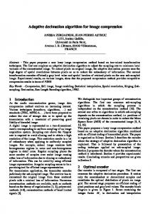
Figure 1.
Subdivide with split planes
Overview of the decimation algorithm.
3 Background
nal mesh). Then an iso-surfacing technique such as marching cubes can be used to extract a surface approximating the original mesh. Rossignac’s method is capable of generating representations at any reduction level. Unfortunately, it is not amenable to a compact progressive operator. For example, if merging neighboring vertices eliminates 1000 triangles, we need to keep track of each triangle modified and its relationship to the merged vertices, and do this for each merging step of the algorithm. Another problem with this method is that points can be merged regardless of surface coherence. For example. points that lie close to one another (measured via Euclidean distance) but are far apart (via surface distance) or even on separate surfaces may be merged. The volume sampling technique can generate representations at almost any level by judicious selection of the sampling (or volume) dimensions. Unfortunately, it is not possible to recover the original mesh using this technique, since the extracted iso-surface has no direct relation to triangles in the original mesh. Also, there is no method to control the number of triangles produced by the method, and the number of triangles may vary unpredictably as the volume dimensions are changed.
In this section we briefly describe some related work that forms the basis of our progressive decimation algorithm.
3.2
3.1
Topology Modifying Algorithms
We began our work by investigating two important polygon reduction algorithms that modify topology. Rossignac [9] uses a vertex merge technique, where local vertices can be identified using an octree or 3D bin array. Vertices lying close to each other are merged into a single vertex, and the topology of the affected triangles are then updated. This may consist of either triangle deletion (if two or three of the vertices are merged), or updating the connectivity list of the triangle. He et al. [10] use a volume sampling approach, where the triangles are convolved into a volume to generate scalar values (e.g., scalar value may be distance from origi-
Decimation
The decimation algorithm has been widely used because of its combination of desirable features: O(n) time complexity, speed, simplicity, and the ability to treat large meshes. In addition, it preserves high-frequency information such as sharp edges and corners, and creates reduced meshes whose vertices are a subset of the original vertex set, thereby eliminating the need to map vertex information. However, as originally presented the decimation algorithm is topology preserving and provides no progressive mesh representation. The decimation algorithm proceeds by iteratively visiting each vertex in the triangle mesh. For each vertex, three basic steps are carried out. The first step classifies the local geometry and topology in the neighborhood of the vertex. The clas-
sification yields one of the five categories shown in Figure 1: simple, boundary, complex, edge, and corner vertex. Based on this classification, in the second step a local planarity measure is used to determine whether the vertex can be deleted. Although many different criterion are possible, distance to plane (for simple vertices) and distance to line (for edge and boundary vertices) has proven to be useful. If this decimation criterion is satisfied, in the third step the vertex is deleted (along with associated triangles), and the resulting hole is triangulated. The triangulation process is designed to capture sharp edges (for vertices classified edge and corner) and generally preserve the original surface geometry. (See [1] for additional details.) An attractive feature of the decimation algorithm is its relative speed. We used the decimation algorithm as the basis on which to build our progressive algorithm.
3.3
Progressive Meshes
A progressive mesh is a series of triangle meshes i i M = M ( V , K ) related by the operations n
ˆ = M )→M (M
n–1
1
→…→M →M
0
(1)
n
ˆ and M represent the mesh at full resolution, where M 0 and M is a simplified base mesh. Here the mesh is 3 defined in terms of its geometry V , or vertex set in R , and K is the mesh topology specifying the connectivity of the mesh triangles. It is possible to choose the progressive mesh operations in such a way to make them invertible. Then the opera0 tions can be played back (starting with the base mesh M ) 0
1
M →M →…→M
n–1
→M
n
(2)
to obtain a mesh of desired reduction level (assuming that 0 the reduction level is less than the base mesh M ). Hoppe’s invertible operator is an edge collapse and its inverse is the edge split (Edge Collapse/Split) shown in Figure 5(a). Each collapse of an interior mesh edge results in the elimination of two triangles (or one triangle if the collapsed vertex is on a boundary). The operation is represented by five values Edge Collapse/Split (v s, v t, v l, v r, A )
where v s is the vertex to collapse/split, v t is the vertex being collapsed to / split from, and v l and v r are two additional vertices to the left and right of the split edge. These two vertices in conjunction with v s and v t define the two triangles deleted or added. In Hoppe’s presentation, A represents vertex attribute information, which at a minimum contains the coordinates x of the collapsed / split vertex v s . A nice feature of this scheme is that a sequence of these operators is compact (smaller than the original mesh representation), and it is relatively fast to move from one reduction level to another. One significant problem is that the reduction level is limited by the reduction value of the 0 base mesh M . Since in our application we wish to realize any given reduction level, the base mesh contains no triangles
n
ˆ = M )→M (M
n–1
1
0
→ … → M → (M = M (V, ∅))
(3)
(some vertices are necessary to initiate the edge split operations). Thus our progressive mesh representation consists of a series of invertible operations, without requiring any base mesh triangles.
4 Algorithm Our proposed algorithm is based on two observations. First, we recognized that reduction operations (such as edge collapse) reduce the high-frequency content of the mesh, and second, topological constraint can only be removed by modifying the topology of the mesh. The implication of the first observation is that “holes” in the mesh (see Plates 1(a)-(c)) tend to close up during reduction. The only reason they do not close completely is because topological modification is prevented. The second observation led us to realize that we could modify the topology by “splitting” the mesh, i.e., replacing one vertex with another for a subset of the triangles using the original vertex. We also realized that any collection of triangles, whether manifold or non-manifold, could be simplified by splitting the mesh appropriately. Thus we developed our algorithm to use topology-preserving operators whenever possible, to allow hole closing (or non-manifold attachments to form), and to split the mesh when further reduction was not possible.
4.1
Overview
The algorithm is similar to the decimation algorithm. We begin by traversing all vertices, and classify each vertex according to its local topology and geometry. Based on this classification, an error value is computed for the vertex. The vertex is then inserted into a priority queue, where highest priority is given to vertices with smallest error values. Next, vertices are extracted from the priority queue in order. The vertex is again classified, and if of appropriate classification, an attempt is then made to retriangulate the loop formed by the triangles surrounding the vertex. Unlike the decimation algorithm, where the hole is formed by deleting the vertex and triangles, in our algorithm the retriangulation is formed by an edge collapse. Note that in this process holes in the mesh may close, and non-manifold attachments may form. If all allowable triangulations are performed and the desired reduction level is still not achieved, a mesh splitting operation is initiated. In this process, the mesh is separated along sharp edges, at corners, at non-manifold vertices, or wherever triangulation fails (due to no legal edge collapses). This process continues until the desired reduction rate is achieved.
4.2
Vertex Classification
Vertices are classified based on topological and geometric characteristics. Key topological characteristics are whether the vertex is manifold or non-manifold, or whether the vertex is on the boundary of the mesh. A man-
Simple
Boundary
Non-manifold ei ej
Error = ei + ej Σek
Error = ei + ek
type of Crack Tip
Figure 2.
Interior Edge
Corner
Degenerate
Vertex classification. Crack tip vertices shown displaced to emphasize topological disconnect.
ifold vertex is one in which the triangles that use the vertex form a complete cycle around the vertex, and each edge attached to the vertex is used by exactly two triangles. A boundary vertex is used by a manifold semi-cycle (i.e., two of the edges on the mesh boundary are used by only one triangle). Note that a vertex with a single triangle attached to it is a boundary vertex. A vertex not falling into one of these two categories is classified non-manifold. Geometric characteristics further refine the classification. A feature angle (angle between the normals of two edge-connected triangles) is specified by the user. This parameter is used to identify sharp edges or corners in the mesh, and guide the triangulation process. Whether a triangle is degenerate is another important geometric characteristic. A degenerate triangle is one that has zero area, either because two or more vertices are coincident, or because the vertices are co-linear. (Although not common in most meshes, many CAD systems do produce them.) Proper treatment of degenerate triangles is necessary to implement a robust algorithm. Vertices are classified into seven separate categories as shown in Figure 2. There are three base types: simple, boundary, non-manifold; and four types derived from the three base types: corner, interior edge, crack-tip, and degenerate. Interior edge vertices have two feature edges, and corner vertices have three or more feature edges (if simple), or one or more feature edges (if a boundary vertex). Crack-tip vertices are types of boundary vertices, except that the two vertices forming the boundary edges are coincident. These form as a side effect of some splitting operations. These types must be carefully treated during triangulation to prevent the propagation of the crack through the mesh.
4.3
Error Measures
The computation of vertex error is complicated by the fact that the topology of the mesh is changing. Researchers such as [8] and [11] have devised elaborate techniques to limit the global error of a reduced mesh, but these methods depend on the topology of the mesh remaining constant. When the topology changes, it is hard to build useful simplification envelopes or to measure a distance to the mesh surface. Because of these considerations, and
Error distributed to surrounding vertices
ei
Figure 3.
Computing and distributing error.
because of our desire for rapid decimation rates, we choose to retain the distance to plane and distance to line error measure employed in the decimation algorithm (Figure 1). Our only modification to the process is to estimate the error of a vertex connected to a single triangle differently. Instead of using distance to line that a boundary vertex would use, we compute an vertex error e i based on the triangle area a i ei =
ai
(4)
which is an effective edge length. This error measure has the effect of eliminating small, isolated triangles first. One improvement we made to the process of error computation is to distribute and accumulate the error of each deleted vertex. The idea is as follows: we maintain an accumulated error value e i for each vertex v i . When a vertex v j connected to v i is deleted via an edge collapse, the error e j is distributed to v i using ei = ei + e j
(5)
Thus the total error e i is a combination of the local error (i.e., distance to plane or distance to edge measure) plus the accumulated error value at that vertex. The error at each vertex is initially zero, but as the mesh is reduced, regions that are non-planar will generate errors, and therefore propagate the error to neighboring vertices. Figure 3 illustrates this process or a 1D polyline and 2D surface mesh. A nice feature of this is approach is that it is relatively simple to compute a global error measure. As a vertex is deleted and the hole re-triangulated, the actual error eˆ j to the re-triangulated surface (versus the estimated error e j ) is computed. (The error eˆ j is computed by determining the minimum distance from the deleted vertex to the re-triangulated surface.) Then, the accumulated error is actually a global error bounds. This global error measure is conservative, but it can be used to terminate the algorithm for applications requiring a limit on surface error. (Note: setting a limit on maximum error may prevent the algorithm from achieving a specified reduction value.)
4.4
Priority Queue
A central feature of the algorithm is the use of a priority queue. We use an implementation similar to that described by [5], but modified to support the Delete(id) method,
Root Level 1 Children
Array tree implementation
Index into tree based on id
( e i, v i ) 0
j ( v0 ) = 2
( e i, v i ) 1
j ( v1 )
( e 0, v 0 ) 2
j ( v2 )
…
…
( e i, v i ) m – 1
j ( vn – 1 )
( e i, v i ) m
j ( vn )
vs vl v4 v3 v2
3 lr
vr
Collapse
vt
Split
vr vt
vl
a) An edge collapse and split
= ( v 1, v 5, v 4, v 3 ) v5 4 ll
4
Invalid
lr
vt = v1
3
Figure 4.
Modified priority queue implementation.
where id specifies a vertex not necessarily at the top of the queue. The implementation is based on a well-balanced, semi-sorted binary tree structure, represented in a contiguous array. In addition, we have another array indexed by vertex id, that keeps track of the location of a particular id in the priority queue array. Figure 4 illustrates the data structure. (Note that the introduction of the priority queue means the time complexity of the algorithm is O(n log n) as compared to the O(n) of the decimation algorithm.) The addition of the Delete(id) method is necessary because of the incremental nature of the progressive decimation algorithm. When a vertex is deleted (via an edge collapse), both the local topology and geometry surrounding the vertex are modified. The effect is that the vertices directly surrounding the deleted vertex (i.e., those connected by an edge) have their topology and geometry modified as well. Thus the error values of these vertices must be recomputed. This means that the surrounding vertices are first deleted from the queue, the error is recomputed, and the vertices are reinserted back into the priority queue.
4.5
Triangulation
A vertex marked for deletion is eliminated by an edge collapse operation as shown in Figure 5(a). We identify the edge to collapse (and the vertex v t ) by identifying the shortest edge ( v s, v t ) that forms a valid split. If feature edges are present, we choose the shortest feature edge. This is not an optimal scheme, but when used with small feature angle values gives satisfactory results. We chose this simple approach because of our requirements on triangle processing rate. A valid split is one that creates a valid local triangulation (i.e., triangles do not overlap or intersect). The edge collapse may modify the global topology of the mesh, either by closing a hole or introducing a non-manifold attachment. Non-manifold attachments may occur, for example, when a vertex at the entrance of a tunnel is deleted, and the tunnel entrance collapses to a line. (See Figure 5(c) and (d).) We use a half-space comparison method to determine whether an edge collapse is valid. To determine if a vertex v 1 = v t forms (in conjunction with v s ) a valid split, we define the loop of vertices connected to v s as L i = ( v 1, v 2, …, v n ) . An edge collapse is valid when all
l l = ( v 1, v 3, v 2 )
b) Valid and invalid splits
c) Closing a hole
d) Forming non-manifold attachment
Figure 5.
Triangulation via edge collapse
planes p i passing through the vertices ( v t, v j ) for 3 ≤ j ≤ n – 1 and normal to the average plane normal N i separate the vertex loop l i into two non-overlapping subloops. This comparison can be computed by creating the n – 3 split planes and evaluating the plane equation p i = N i ⋅ ( v j – v t ) . The sub-loops are non-overlapping when all vertices in one sub-loop evaluate either positive or negative, and all vertices in the other loop evaluate to the opposite sign. As we mentioned earlier, crack-tip vertices must be carefully triangulated to avoid propagating a crack through the mesh. Crack-tip vertices are treated like simple vertices by temporarily assuming that the two coincident vertices are one vertex. Then, if a valid split can be found, the two coincident vertices are merged with a VertexMerge, followed by an EdgeCollapse. Although this may reverse a previous VertexSplit operation, it does eliminate a vertex and two triangles and prevent the crack from growing. Eventually changes in the local topology and geometry will either force the crack to grow or to close up. The process will eventually terminate since the mesh will eventually be reduced to a desired level, or will be eliminated entirely.
4.6
Vertex Splits
A mesh split occurs when we replace vertex v s with vertex v t in the connectivity list of one or more triangles that originally used vertex v s (Figure 6(a)). The new vertex v t is given exactly the same coordinate value as v s . Splits introduce a “crack” or “hole” into the mesh. We prefer not to split the mesh, but at high decimation rates this relieves topological constraint and enables further decimation.
vr vs vl
Split
vs Merge
vr vt
vl a) A vertex split and merge
Interior Edge
Non-manifold
Corner
Other types
b) Splitting different vertex types
Figure 6.
Mesh splitting operations. Splits are exaggerated.
Splitting is only invoked when a valid edge collapse is not available, or when a vertex cannot be triangulated (e.g., a non-manifold vertex). Once the split operation occurs, the vertices v s and v t are re-inserted into the priority queue. Different splitting strategies are used depending on the classification of the vertex (Figure 6(b)). Interior edge vertices are split along the feature edges, as are corner vertices. Non-manifold vertices are split into separate manifold pieces. In any other type of vertex splitting occurs by arbitrarily separating the loop into two pieces. For example, if a simple vertex cannot be deleted because a valid edge collapse is not available, the loop of triangles will be arbitrarily divided in half (possibly in a recursive process). Like the edge collapse/split, the vertex split/merge can also be represented as a compact operation. A vertex split/ merge operation can be represented with four values Vertex Split/Merge (v s, v t, v l, v r )
as shown in Figure 6(a). The vertices v l and v r define a sweep of triangles (from v r to v l ) that are to be separated from the original vertex v s (we adopt a counter-clockwise ordering convention to uniquely define the sweep of triangles).
4.7
Progressive Mesh Storage
The storage requirements for a progressive mesh are smaller than the standard triangle mesh representation schemes. We estimate the storage requirements as follows. A mesh generally consists of about n vertices and 2n triangles, for a total of 9n words of storage using a standard scheme of three vertex indices per triangle, and three coordinate values per vertex, each stored as one word of information. Using a progressive mesh representation, each edge split requires at a minimum the coordinates and vertex indices v s , v t , v l , and v r , and creates two triangles and one vertex, at a cost of 7n words of storage. A vertex split requires the four vertex indices v s , v t , v l , and v r , and typically no more than n ⁄ 4 splits are required to 0 reduce the mesh to M . We can then estimate the storage
requirements to total 8n words, for a savings of 11% over the standard scheme. Note that even though the vertex split requires additional storage over edge collapse, it does allow us to virtually eliminate the cost of representing the base mesh. Further savings are possible by carefully organizing the order of the playback operations. For example, by renumbering the vertices after the forward progression is complete, it is possible to eliminate the vertex index v t . As [7] describes, additional storage savings are possible based on the coherence of local topological operations, and by 16-bit quantization and compression of the coordinate values. We can also take into account the number of bits required for a vertex index and use smaller word sizes, if appropriate.
4.8
Error Inflection Points
An error inflection point E i occurs when the ratio of the error is greater than a user-defined value E r ei + 1 ----------- > E r ei
(6)
The importance of inflection points is that they mark abrupt transitions in the error of the mesh, and often correspond to significant changes in the appearance of the mesh. Thus, by tracking these inflection points, we can find natural points at which to generate LOD’s for a particular part. For example, the first error inflection point always occurs at the point in which non-zero error is introduced. Geometrically, this corresponds to the point where all co-planar triangles have been removed from the interior of the mesh, and all co-linear vertices are removed from the boundary of the mesh. This is an important point in the reduction process, since at this point the reduced model is indistinguishable from the original mesh using typical surface-shading techniques. We use error inflection points to build other levels in our sequence of LOD models. For a requested reduction level L k , we use the mesh M j with the closest inflection point M j : E j – L k ≤ E i – L k for all k ≤ i, j ≤ n
(7)
Typical values of E r range from 10 to 100, and are empirically determined.
4.9
A Variation In Strategy
We found a variation of our splitting strategy to work well for a certain class of problems. In this variation, we presplit the mesh along feature edges, at corners, and at nonmanifold vertices. This strategy works well for objects with large, relatively flat regions, separated by thin, small surfaces. This is because splitting isolates regions from one another, thereby preventing the distortion of the mesh due to errors from edge collapse across the thin surfaces. An example of this behavior can be seen in Color Plate 2, where the triangles forming the thin edges of the plate disappear before the much larger triangles forming the faces of the plate.
Model
Number Triangles Shell 1132 Plate 2624 Heat Ex. 11,006 Turbine 314,393 Blade 1,683,472 Figure 7.
Reduction 0.5 time
collapses
splits
0.46 319 0 1.07 656 0 3.27 2759 0 158 98,401 43,011 747 421,042 0
Reduction 0.75 time
collapses
Reduction 0.90
splits
0.68 494 0 1.41 984 0 4.42 4139 0 202 157,877 69,019 825 631,606 0
time
collapses
splits
Reduction 1.00 time
collapses
Rate
splits
0.70 557 0 0.76 648 0 89,368 1.68 1228 169 1.73 1457 221 91,006 5.36 5447 914 5.86 6355 1160 112,689 229 202,702 83,214 241 232,281 88,184 78,272 914 758,056 0 1042 852,743 24,501 96,937
Results for five different meshes. Times shown are elapsed seconds. Number of edge collapses and vertex splits are also shown. The rate is the maximum number of triangles eliminated per elapsed minute.
5 Results We implemented the algorithm as a C++ class in the Visualization Toolkit (vtk) system [6]. The algorithm is relatively compact requiring less than 2 KLines of code (including the priority queue implementation). No formal optimization of the code was attempted other than the usual compiler optimization. All test results are run on a 190 MHz R10000 processor (compiled and run in 32-bit mode) with 512 MBytes of memory. We choose to test the algorithm on five different models. The first two are shown in Color Plates 1 and 2, and are a shell mesh and plate with seven holes. The next two models are extracted from CAD systems. The first is a heat exchanger with 11,006 original polygons. The next is a turbine shell consisting of 314,393 polygons. Finally, the last model is very detailed turbine blade consisting of 1.68 million triangles originally. The data was obtained by generating an isosurface from a 512 x 512 x 300 industrial CT scan of the part. Figure 7 shows elapsed wall clock time in seconds for these five examples at reduction levels of 0.50, 0.75, 0.90, and 1.00 (elimination of all triangles). We also show the number of edge collapses and vertex splits required at each level of reduction. Color Plates 3(a)-(f) show results for the heat exchanger. Plates 4(a)-(f) show results for the turbine shell. Plates 5(a)-(f) show the results for the turbine blade. Note that in each case the onset of vertex splitting is shown. In some of these color plates the red edges are used to indicate mesh boundaries, while light green indicates manifold, or interior edges. The ability to modify topology provides us with reduction levels greater than could be achieved using any topology preserving algorithm. Color Plate 4 clearly demonstrates this since the maximum topology preserving reduction we could obtain was r=0.404. We were able to more than double the reduction level and still achieve a reasonable representation. At extreme reduction levels the quality of the mesh varied greatly depending on the model. In some cases a few large triangles will “grow” and form nice approximations (e.g., the plate and shell). In other cases, the mesh is fragmented by the splitting process and does not generate larger triangles or good approximations. But in each case we were able to recognize the part being represented,
which is sufficient for initial camera positioning and navigation. We were generally pleased with the results of the algorithm, since the creation of non-optimal meshes is well balanced by the algorithm’s speed, ability to process large meshes, and robustness.
6 Conclusion We have described a topology modifying decimation algorithm capable of generating reductions at any level. The algorithm uses the invertible progressive operators Edge Collapse/Split and Vertex Split/Merge to construct compact progressive meshes. The algorithm has a high enough polygonal processing rate to support a large scale design and visualization process. We have found it to be an invaluable tool for creating LOD databases.
References [1] [2] [3]
[4] [5] [6]
[7] [8]
[9]
[10]
[11] [12]
W. J. Schroeder, J. A. Zarge, and W. E. Lorensen. Decimation of triangle meshes. Computer Graphics 26(2):65-70, July 1992. Turk, G. Re-Tiling of polygonal surfaces. Computer Graphics, 26(2):55-64, July 1992. H. Hoppe, T. DeRose, T. Duchamp, J. McDonald, W. Stuetzle. Mesh optimization. Computer Graphics Proceedings (SIGGRAPH ‘93), pp 19-26, August 1993. P. Hinker and C. Hansen. Geometric optimization. In Proc. of Visualization ‘93. pages 189-195, October 1993. A. V. Aho, J. E. Hopcroft, J. D. Ullman. Data Structures and Algorithms. Addison-Wesley, 1983. W. J. Schroeder, K. M. Martin, W. E. Lorensen. The Visualization Toolkit An Object-Oriented Approach To 3D Graphics. PrenticeHall, 1996. H. Hoppe. Progressive Meshes. Proc. SIGGRAPH ‘96, pp 99-108, August 1996. J. Cohen, A. Varshney, D. Manocha, G. Turk, H. Weber, P. Agarwal, F. Brooks, W. Wright. Simplification envelopes. Proc. SIGGRAPH ‘96, pp 119-128, August 1996. J. Rossignac and P. Borel. Multi-resolution 3D approximations for rendering. In Modeling in Computer Graphics, pp. 455-465, Springer-Verlag, June-July 1993. T. He, L. Hong A. Kaufma, A. Varshney, S. Wang. Voxel based object simplification. In Proc. of Visualization ‘95, pp. 296-303, October 1995. R. Klein, G. Liebich, W. Strasser. Mesh reduction with error control. In Proc. of Visualization ‘96, pp. 311-318, October 1996. P. Heckbert and M. Garland. Fast polygonal approximation of terrains and height fields. Technical Report CMU-CS-95-181, Carnegie Mellon University, August 1995.
a) Original model 1,132 triangles
b) Topology unchanged 43 triangles
c) Topology modified
Plate 1 - Topological constraints prevent further reduction (shell with holes). Red edges are on the boundary of the mesh, light green edges are in the interior of the mesh.
a) Original model 2,624 triangles
b) Shortly after splitting 157 triangles
c) Final model 4 triangles
Plate 2 - Sharp edge splits and hole elimination (thin plate with holes). (b) is a close-up of the mesh showing the how the hole triangles are disconnected from the top plate.
a) Original model 11,006 triangles
b) Reduction 50%, 5,518 triangles
c) Just after mesh splitting 2,707 triangles, 75.4% reduction
d) Reduction 90%, 1,100 triangles
e) Reduction 95%, 550 triangles
f) Reduction 98%, 220 triangles
Plate 3 - Heat exchanger at different levels of reduction. (c) shows the edges that are split at the onset of edge splitting.
a) Original model 314,39 triangles
b) Shortly before splitting 187,449 triangles, reduction 40.4%
c) 50% reduction, 157,196 triangles
d) 75% reduction, 78,598 triangles
e) 90% reduction, 31,439 triangles
c) 95% reduction, 15,719 triangles
Plate 4 - Turbine shell shown at various reduction levels. Shell has thickness, and many features requiring vertex splitting.
a) Original model 1,683,472 triangles
b) Close-up of edges showing holes leading to interior
c) 75% reduction, 420,867triangles
d) Shortly before splitting 134,120 triangles, 92% reduction
e) 95% reduction, 84,173 triangles
f) 99.5% reduction, 8,417 triangles
Plate 5 - Turbine blade shown at various levels of reduction. Data derived from 5122 by 300 CT scan.