Interactive Digital Media R&D Program, under research grant NRF2008IDM- ... convert daily objects into a touch pad. ..... This signature is obtained during.
A TOUCH INTERFACE EXPLOITING THE USE OF VIBRATION THEORIES AND INFINITE IMPULSE RESPONSE FILTER MODELING BASED LOCALIZATION ALGORITHM Kirill Poletkin, XueXin Yap and Andy W. H. Khong Nanyang Technological University, Singapore Email: {kpoletkin, xxyap, andykhong}@ntu.edu.sg ABSTRACT Research into human-machine computer interface (HMI) has been very active in recent years due to the proliferation and advances in software applications. Such devices are aimed at providing a more natural interface for which humans and machines interact. In this multi-disciplinary research, we propose a new approach to the development of a touch interface through the use of surface mounted sensors which allow one to convert hard surfaces into touch pads. We first develop, using mechanical vibration theories, a mathematical model that simulates the output signals derived from sensors mounted on a physical surface such. Utilizing this model, we show that the profile of the output signals is unique not only in time but also in the frequency domain. We then exploit this important property to localize finger taps by developing a source localization algorithm based on infinite impulse response filter model for location template matching. The performance of the proposed algorithm is compared with existing approaches and verified both in a synthetic as well as a real environment for the localization of a finger tap on a touch interface. Keywords— touch interface, location template matching, impact on plate, accelerometer. 1. INTRODUCTION The personal computer (PC) have become an integral part of modern life. It is difficult to imagine the field of human activities that can do without these remarkable machines. Current approaches for human-machine interface (HMI) technology rely on the need for input devices such as the alphanumeric keyboard and the optical pointing device. As new interactive digital media software applications continue to evolve over the years, one of the main drawbacks of such input devices is that they impede ease of operating software or manipulating data which require complex user input operations. As a result, the use of keyboards or mouse limit, to a significant extent, the scope, functionality as well as ease of use of the PC. Such limitation can be addressed by touch screens which have been employed in, for example, portable devices such as smartphones and GPS devices. Such This work is supported by the Singapore National Research Foundation Interactive Digital Media R&D Program, under research grant NRF2008IDMIDM004-010.
c 978-1-4244-7493-6/10/$26.00 2010 IEEE
touch sensitive screens often employ capacitive sensing technologies where the distortion of an electrostatic field is detected by a change in capacitance on the touch surface for the purpose of finger tap localization. Although this proven technology has gained much popularity in recent years, its high implementation cost limits the size of the screens. As a result they are often limited to small portable devices. In order to address this problem, one solution which has recently attracted attention in the research community is the development of a touch interface (TI) platform that allows one to convert daily objects into a touch pad. This technology is based on the deployment of surface mounted sensors as well as acoustic localization of a tapping source on the surface of a physical object. In particular, the TI considered in [1] describes impact localization methods based on well-known techniques such as time-differences-of-arrival and location template matching. The effectiveness of both methods has been verified experimentally for isotropic [2] as well as anisotropic [3] materials. Although some progress has been made pertaining to the localization of finger taps on hard surfaces such as wood and glass for TIs, localization using signals received by the sensors mounted on such surfaces present huge challenges. These challenges, which affect the accuracy of source localization to a large extent, include temperature variation, various types of wave propagation, multipath propagation of these waves through the anisotropic solid surface as well as variation of propagation speed due to dispersive effects of the channel between the finger tap and the sensor. Due to the complexity of the problem, results presented thus far have been focused on improving the accuracy of the source localization algorithms albeit in a relatively ad-hoc manner. In this work, we propose a novel approach to the development of source localization algorithms for a TI that employs surface mounted sensors which in turn allow one to convert any hard surfaces into a touch pad. In this inter-disciplinary research, we first develop, using mechanical vibration theories, a mathematical model that simulates the output signals derived from sensors mounted on a physical surface. Utilizing this model, we show that the profile of the output signals is unique in the frequency domain. This important property is then employed to localize finger taps by developing a source localization algorithm based on an infinite impulse response filter (IIRF) modeling for location template matching (LTM). The
ICME 2010
Sensor
V1 V2
(xs,ys)
…
V5
Nm(t)
Human Touch
…
4 cm
V6
Hardware part of touch interface
Acrylic Panel
V25
V21
x
Normalized Amplitude
N0(t) x0 , y0
Lx
hm(n)
Source localization algorithm
Sensors
L Ly
4 cm
Presonus Firestudio 2626
Physical object
Mathematical model of physical object
Computer
Fig. 1. Diagram of TI with a matrix of predefined points. performance of the proposed algorithm is compared with existing approaches and verified both in a synthetic as well as a real Time (s)of a finger tap on a TI. environment for the localization
In this work, we consider a rectangular plate; one of the most common structure that covers a wide range of objects such as tables, walls, and glass windows. As shown in [4] the response
Sensor Output
of the plate due to an impact can be represented by classical plate theory. Defining P (x, y, t) as the pressure at a (x, y) location on the plate at time instance t, the vertical displacement w(x, y, t) of the plate at any (x, y) location must satisfy the following motion equality P (x, y, t)
=
dw(x, y, t) + dt d2 w(x, y, t) ρLz , dt2
D∇4 w(x, y, t) + µ
(1)
where µ is absorption coefficient, ρ is the density, Lz is the thickness of the plate, D = EL3z /(1 − ν 2 ), E is the Young’s ∂4 ∂4 ∂4 modulus, ν is Poisson’s ratio while ∇4 = ∂x 4 + 2 ∂x2 ∂y 2 + ∂y 4 . In order to solve for (1), we first note that a point impact at finger location (x0 , y0 ) can be expressed as P (x, y, t) = N0 (t)δ(x − x0 )δ(y − y0 ),
(2)
where δ(x), and δ(y) are the Dirac delta functions. By substituting (2) into (1), the solution of (1) in the complex domain for zero initial condition become w(x, y, s) = Wp (x, y, x0 , y0 , s)N0 (s),
(3)
where s is Laplace variable, N0 (s) is Laplace transform of function N0 (t). The variable Wp (x, y, x0 , y0 , s) is the transfer function of the physical object which is in the form of Wp (x, y, x0 , y0 , s) =
∞ X ∞ X l=1 b=1
Wlb 4 2 , (4) ρLz Lx Ly s2 + µ es + ωlb
where Wlb ωlb
2.1. Mathematical model of surface vibration on solids
Mathematical model of sensor
Fig. 2. Block diagram of touch interface.
2. MATHEMATICAL MODEL OF HUMAN-COMPUTER TOUCH INTERFACE In view of the above, the TI system can be represented as shown in Fig. 1 which consist of an interactive physical surface, a surface-mounted sensor, and a PC which processes signals received from these sensors. The interaction of human with this interface is realized by means of an impact due to the finger on the physical surface. The aim of this work is therefore to estimate the location of this finger tap from the received signals. To achieve this, we first define a coordinate frame as shown in Fig. 1 where the origin is located at the left top corner of the plate. The coordinates of a finger impact N0 (t) are denoted by x0 and y0 . The impact excites mechanical waves which are detected by the surface-mounted sensor at coordinates (xs , ys ). The mechanical waves are then converted by these sensors into electrical signals which are subsequently processed by the source localization algorithm on the PC for the control of software applications. We now present a model that exploits the mechanics of vibrating waves which provides an insight into the properties of wave propagation through solids. This in turn can be employed for the development of source localization algorithms presented in subsequent sections. As can be seen in Fig. 2, this model comprises of models for the physical object and the sensor. The aim of these blocks is to transform a human touch into electrical signals. Since different types of sensors such as accelerometers, optical sensors and strain gauges can be used to detect mechanical wave propagation in solids, a transforming block is included to serve as a link between the physical object and sensor models.
Transforming block
αl
=
sin(αl x) sin(βb y) sin(αl x0 ) sin(βb y0 ), � 2 �s l b2 D 2 = π + 2 , 2 Lx Ly ρLz
(5)
= πl/Lx , βb = πb/Ly ,
(7)
(6)
such that µ e = µ/(ρLz ) is the reduced coefficient of absorption and that l, b ∈ Z+ are the modes of wave propagation.
-2
2.3. Model between impact and sensor output Having described the physical object and sensor model, we now integrate these models to formulate the transfer function between the impact and the output of the accelerometer. It is important to note that since we are using an accelerometer, the vertical displacement at the sensor location must be transformed into acceleration by means of s2 . Thus, the transfer function between the impact and the sensor output is given by (10)
where xs , ys are the coordinates of the accelerometer. It is therefore important to see that (10) is not just a function of the location of the finger tap but also a function of frequency via the Laplace variable s. As will be shown in Section 3, we utilize this property for the localization of our finger tap. 2.4. Illustrative example using the mathematical model We now provide an illustrative example of how the model can be utilized to understand properties of the received signals. We begin by first defining, for the Murata shock sensor, a time constant T = 7.1×10⁻⁷ s, a relative damping coefficient of ζ = 0.1 and a gain coefficient of Ks = 3.5 × 10⁻³ V/(ms−2 ). These values have been selected to match the frequency response of the sensor found in its datasheet [6]. We further proceed by defining properties of a surface with dimensions given by 80 × 80 × 0.52 cm. For this illustrative example, we chose plastic with the following properties: E = 69 × 109 Pa, ν = 0.35,
0.06
Impact 2
2 0 -2 -4 0
0.02 0.04 Time (sec)
0.06
Fig. 3. Output signals of sensor to first and second impacts. Figure 3 shows the output of the signals received by the sensor from the first two impacts. For clarity of presentation, we choose to only show the outputs of these two impacts. As can be seen, the signals exhibit some form of damping particularly after 5 ms. This is due to the frequency dependency nature of the signal given by (10). The magnitude spectrum of these signals is given in Fig. 4. As can be seen, these output signals include a high frequency component that is due to resonant frequency of the accelerometer at approximately 2 kHz. In addition, the spectrum profile of each received signal is unique. This occurs particularly for frequencies lower than 500 Hz which are caused by the resonant frequencies of the material used in this simulation example. This important property is exploited in an IIRF-based algorithm for source localization. 1
1
Impact 1 Impact 2
0.8
Power
Ks Y (s) = 2 2 , (9) G(s) T s + 2ζT s + 1 q where Ks is the gain coefficient, T = M k is the time constant µ and ζ = 2√M k is the relative damping coefficient. Ws (s) =
0.02 0.04 Time (sec)
4
Sensor Output, V
0
(8)
where u(t) is the output of accelerometer, g(t) is the input acceleration, M is the proof mass, ς is the damping coefficient, and k is the stiffness of the spring element. The corresponding transfer function is then given by
Impact 1
2
-4 0
du(t) d2 u(t) +ς + ku(t) = g(t), M dt2 dt
Uout (xs , ys , s) = Ws (s)s2 Wp (xs , ys , x0 , y0 , s), N0 (s)
4
0.6 0.4 0.2 0 0
Impact 3 Impact 4
0.8
Power
There are various types of sensors including optical sensors and strain gauges that can detect vibrational waves on hard surfaces. One of the most cost effective solution is the use of surface mounted accelerometers which can be deployed to, for example, localize impacts. The shock accelerometer is a simple wave propagation detection sensor. This shock accelerometer is characterized by the frequency response, with its output voltage dependant on the input acceleration. The behavior of an such a sensor can be described by a second-order linear differential equation of the form [5]
and ρ = 2710 kg/m3 . In this synthetic simulation, a Murata shock sensor is placed at (0.3, 0.2) m. The coordinates of four impacts are (0.12, 0.12) m, (0.12, 0.68) m, (0.68, 0.68) m, and (0.68, 0.12) m. We have also used l = b = 3.
Sensor Output, V
2.2. Mathematical model of accelerometer
0.6 0.4 0.2
1000
2000 3000 Frequency (Hz)
4000
0 0
1000
2000 3000 Frequency (Hz)
4000
Fig. 4. Spectrum of sensor output for difference impacts.
3. SOURCE LOCALIZATION USING LTM ALGORITHM In order to develop the proposed IIRF-based location template matching (LTM) algorithm, we first examine the working principle behind LTM. We consider a single-input-single-output (SISO) system as shown in Fig. 1 where N0 (t) is the source signal while u(n) = [u(n), . . . , u(n + Lu − 1)]T is defined as the received signal given that Lu is the length of u(n). The aim of LTM is then to estimate the source location using u(n). To achieve this, LTM requires prior knowledge of the source signature at a particular location. This signature is obtained during the training phase where we define
Normalized Amplitude
Normalized Amplitude
1 0.5 0 -0.5 -1
0
0.005
0.01
0.015
0.02
3.1. Proposed IIRF Model based algorithm for LTM
1 0.5 0 -0.5 -1
0
Time (s)
0.005
0.01
0.015
0.02
Time (s)
Fig. 5. Signal received at sensor from tap made at positions V1 and V2 . hm (n) = [hm (n), . . . , hm (n + Lh − 1)]T
(11)
as the pre-recorded sequence of length Lh for a source location at position index m. In order to estimate the location of the source, one of the recently developed algorithms [7] involves cross-correlating the received signal u(n) with hm (n) such that the estimated location is given by m b corresponding to the highest correlation. In the frequency domain, this correlation can be de� �T scribed by first defining u(ωk ) = F uT (n) 0TLh −1 as the Fourier transform of the zero-padded received signal where F is the (Lu + Lh − 1) × (Lu + Lh − 1) Fourier transform matrix and ωk is the frequency-bin index while 0Lh −1 is the e m (n) = [hm (n + (Lh − 1) × 1 null vector. We next define h T Lh − 1), . . . , hm (n)] as the time-reversed pre-recorded signal such that its zero-padded Fourier transform is given by iT h e (ωk ) = F h e T (n) 0T h . The correlation between rem m
Lu −1
ceived signal u(n) and the pre-recorded signature hm (n) for location m is then given by
cm (p)
= =
[. . . , cm (−1), cm (0), cm (1), . . .]T o n e (ωk ) , F−1 u(ωk ) h m
p,m
= u(n) − u b(n)
e(n)
= u(n) −
I X
a(i)u(n − i),
(14)
i=1
where I is the prediction order and a(i) is the ith filter coefficient. To illustrate the motivation behind this approach, we evaluate a(i) for two instances of received signals u(n) with the taps made at V1 :(41, 20) cm and V2 :(42, 20) cm and the sensor mounted at (5, 25) cm. We then modeled the signal using an IIRF order of I = 3. Figure 6 shows the spectrum plot of the coefficients a(i) for each of these positions when they are evaluated around the unit circle. The vertical lines are plotted by evaluating the pole positions on the unit circle. The top and bottom panels each illustrates the spectrum plotted using fastFourier transform (FFT) for both taps made at positions V1 and V2 respectively. As can be seen, the spectrum plot of a(i) peaks at the dominant frequencies of the received signal. To illustrate this important property mathematically, we first define ω = 2πf /fs with fs being the sampling frequency and f being the frequency of the signal. The spectrum of the time domain signal u(n) is given by
(12)
where p = . . . , −1, 0, 1, . . . is defined as the sample-lag between the two signals u(n) and hm (n) and that is defined as the Sch¨ur product. Utilizing this correlation, the LTM algorithm [7] [8] estimates the location of the acoustic source given by m b corresponding to the maximum cm (p) over all lags p and positions m, i.e., m b = max cm (p).
We now propose a pattern recognition approach to source localization which employs an IIR filter. This approach is chosen over other popular sound recognition techniques such as [9], since those techniques usually model the way the human ear respond to sounds, which might not be applicable for our touch interface. In addition, such methods are often computationally expensive. In view of this, we exploit the all-pole model to extract the dominant frequencies of the received signal by minimizing the error difference of the received signal u(n) and predicted signal u b(n). This prediction error is given by
(13)
The performance of the cross-correlation based LTM algorithm [7] [8] relies on the disparity between impulse responses from each tap location to each sensor. Due to this disparity, neighboring finger tap locations will generate similar yet different responses at the sensors. It has been shown in [7] [8] that location estimation using this correlation based LTM approach allows one to achieve a localization accuracy of ±1.5 cm. However it is important to note that signals u(n) and hm (n) are generated on the same surface, under the environmental conditions that are not vastly different.
|U (ejω )|2 =
|1 +
a(1)e−jω
σe2 , + . . . + a(I)e−jIω |2
(15)
with σe2 being the variance of e(n) where a(i), i = 1, . . . , I can be estimated from its past samples u(n − i). By factorizing the denominator of the function, we can obtain
|U (ejω )|2 =
σe2 . |(ejω − ejω1 ) . . . (ejω − e−jωI )|2
(16)
Hence, we see that U (ejω ) peaks at frequencies ω1 , . . . ωI . Since ω = 2πfi /fs , we can obtain the dominant frequencies. As can be seen from Fig. 6, the dominant frequencies are identified by the all-pole filter coefficients a(i) for both locations V1 and V2 . More importantly, we note that these dominant frequencies differ from each other and we employ this diversity to estimate the source position. To exploit this diversity, the sum of the errors between the filter coefficients of the received signals and those from our
X: 1918 Y:-5
dB
0
using IIRF method using FFT Spectral Peaks
X: 6405 Y: -15
-20 -40 -60
0
2000
4000
6000
8000
10000
12000
Frequency (Hz) 20
X: 1825 Y:-5
dB
0
using IIRF method using FFT Spectral Peaks
X: 5757 Y: -20
-20 -40 -60
0
2000
4000
6000
8000
10000
12000
Frequency (Hz)
Fig. 6. Spectrum overlayed with IIRF model of taps made at V1 and V2 , for I = 3.
pre-recorded signals hm (n) are computed. Defining au (i) and ahm (i) as the filter coefficients computed from the received signal u(n) and the pre-recorded signal hm (n) respectively, this difference is obtained using Sm =
I X
(au (i) − ahm (i))2 .
In a similar manner to LTM employing correlation as described in Section 3, the IIRF-based approach then estimates the location of the source given by m
100
(17)
i=1
m b = min Sm .
a piece of acrylic of dimension 60 × 30 × 0.7 cm. We have positioned the sensor away from the axis of symmetry so as to avoid similarities of the spectrum brought about by this symmetry. Twenty-five tap points, each spaced 1 cm apart, were selected for the training of the database. The first tap point, V1 , is positioned at (41, 20) cm on the acrylic sheet. As seen in Fig. 1, the sensor is marked with a ‘◦’ and each tap point is marked with a ‘•’. The ‘×’ is used to denote the input N (t) that was made on each of the tap points. The tap points are sequentially tapped and digitized using a Presonus Firestudio; the signals were sampled at 24 kHz with 16 bits resolution. These signals are first saved into a database denoted by hm defined in (11). In an earlier experimentation phase, the cross-correlation approach to LTM was found to yield an accuracy of about 68 %. This is because the pre-recorded signals are in the first place very similar. Hence the cross-correlation approach to LTM is unable to distinguish minor amplitude changes in the frequency domain especially when the changes are not of the fundamental frequency. An example of the signals that cross-correlation approach is not able to distinguish are the taps made at V1 and V2 , which gave us the motivation to explore a frequency domain approach to the problem.
(18)
It is worthwhile to note that the computational complexity of the proposed IIRF-based LTM algorithm is substantially lower than that of the cross-correlation based LTM approach. It is noted that of the cross-correlation based LTM algorithm comprises of cross-correlation and a decision step. As has been shown in Section 3, the computation of the cross-correlation requires the Fourier transform, multiplication as well as the inverse Fourier transform. The total complexity for the crosscorrelation based LTM algorithm is thus 12LN log2 2LN + 8LN . The IIRF based LTM algorithm consists of the computation of a(i) using the Levinson-Durbin algorithm and a decision step. The total complexity for the IIRF based LTM algorithm is thus 8LN log2 2LN + 4LN + 15. By calculating the complexity of the two algorithms, it was found that the complexity of the correlation-based method is higher than the IIRF model-based method. As an illustrative example, for the case when u(n) is 1000 samples long, the IIRF model-based method requires approximately 50000 less operations than the correlation-based approach. 4. EXPERIMENTAL RESULTS To verify the algorithm’s performance, we set up an experiment deploying a Murata PKS1-4A1 shock sensor at (5, 25) cm on
Accuracy (%)
20
90 80 70 60 50
5
10
15 IIR Filter Order
20
25
100
Fig. 7. Variation of accuracy for different IIRF orders. We propose to evaluate the performance of the algorithms by means of a weighted function defined as 1 m b = m, 0.5 m b = m ± 1 cm, (19) b(q) = 0.1 m b = m ± 1.5 cm, 0 otherwise, where b(q) is the score of the q th test tap for q = 1, . . . , Q, with Q being the total number of tap points used for testing the algorithms. By averaging the score Q
bT =
1 X b(q), Q q=1
(20)
the accuracy of the algorithm is obtained. Using this weighting function, twenty taps were made by a human subject using a stylus at each of the twenty-five points in the pre-defined tap region, giving Q = 500, as seen in Fig. 1. The two LTM methods were tested and the results tabulated in Table 1. The empirical result of the accuracy when different IIRF orders were used are plotted in Fig. 7. Figure 7 shows
20 using IIRF method using FFT Spectral Peaks
dB
0 -20 -40 -60
0
2000
4000
6000
8000
10000
12000
Frequency (Hz) 20 using IIRF method using FFT Spectral Peaks
dB
0 -20 -40 -60
0
2000
4000
6000
8000
10000
12000
Frequency (Hz)
Fig. 8. Spectrum overlayed with IIRF model of Taps made at V1 and V2 , for I = 12.
that the ideal IIRF order is I = 3, and it was also found that higher IIRF orders tend to pick up dominant peaks found in the unspecified regions along the frequency range of interest. As can be seen in Fig. 8, where an IIRF order of I = 12 is used, a lower accuracy is achieved by the proposed algorithm. Using I = 3, the results of using cross-correlation and IIRF to perform the localization, as seen in Table 1, are 68.00 % and 96.48 % respectively. From this, we note that even with reduced complexity, the IIRF approach to LTM is able to localize approximately 25 % more accurately than the cross-correlation approach. This improvement can be achieved since both time and frequency components are utilized in the spatial localization of taps.
Table 1. Accuracies obtained using correlation and IIRF-based LTM algo-
5. CONCLUSION We show, in this work, that by exploiting the spectral uniqueness of a tap, we can achieve source localization. This is done by modeling the surface and a vibration sensor mathematically. A multi-disciplinary approach was utilized to study the material and the sensor, as well as to design a localization algorithm. Preliminary results of the TI simulation showed that the spectrum profiles of taps made at different locations were unique. This motivated the use of a spectral-template matching based algorithm. Although the cross-correlation approach was able to localize the taps, it does not exploit the spectral uniqueness of the taps. Thus the IIRF modeling-based algorithm was proposed by modeling the spectral peaks of the received signal and comparing it with a set of pre-recorded signals of known locations. Not only is the uniqueness of the spectrum exploited, the complexity cost of the localization is also reduced. The final result of the proposed IIRF-based algorithm was verified with real experimental data. 6. REFERENCES [1] W. Rolshofen, D. T. Pham, M. Yang, Z. B. Wang, Z. Ji, and M. Al-Kutubi, “New approaches in computer-human interaction with tangible acoustic interfaces,” in Proc. Virtual Int. Conf., IPROMs, Ed., May 2005. [2] C. Bornand, A. Camurri, G. Castellano, S. Catheline, A. Crevoisier, E. B. Roesch, K. R. Scherer, and G. Volpe, “Usability evaluation and comparison of prototypes of tangible acoustic interfaces,” in Proc. 2nd Int. Conf. on Enactive Interfaces, Genoa, Italy, Nov 2005. [3] T. Kundu, S. Das, S. A. Martin, and K. V. Jata, “Locating point of impact in anisotropic fiber reinforced composite plates,” Ultrasonic, vol. 48, pp. 193–201, 2008.
rithms.
LTM Algorithm Accuracy
Cross-correlation 68.00 %
IIRF 96.48 %
More importantly, the improvement in accuracy for the proposed IIRF approach is brought about by the different dominant frequencies that exist for different positions on the acrylic surface. This can be noted from the frequency plots as shown in Fig. 6. As a result of this inconsistency across different positions, we model the signal using an all-pole model and estimate the location of the source by comparing the similarities of the filter coefficients. This has the same effect, to a large extent, of comparing the pole locations around the unit circle. As noted in Section 3, apart from the improved performance, the main advantage of using IIRF to perform the localization is that the number terms used for comparison is significantly reduced. In the case where the sampling frequency is 24 kHz, each of the taps is made of Lu = 1000 samples long. The crosscorrelated signals are therefore 1999 samples long. However in the case of IIRF using the same sampling frequency, the tap signal is now represented by 3 coefficients.
[4] J. Doyle, “Determining the contact force during the transverse impact of plates,” Experimental Mechanics, pp. 68– 72, 1987. [5] R. Pallas-Areny and J. G. Webster, Sensors and signal conditioning. John Wiley & Sons, Inc., 1991. [6] PKS1-4A1 Shock Sensor, Murata Manuf. Co., Ltd. [Online]. Available: http://www.alldatasheet.com/datasheetpdf/pdf/167199/MURATA/PKS1-4A1.html [7] D. T. Pham, M. Al-Kutubi, Z. Ji, M. Yang, Z. Wang, and S. Catheline, “Tangible acoustic interface approaches,” in Proc. Virtual Conf., IPROMs, Ed., May 2005. [8] P. di Milano, “Deliverable 2.6 - Part I technical solutions for the TDOA method,” PoliMi, Deliverable 2.6, Aug 2005. [9] S. Chu, S. Narayanan, and C. C. J. Kuo, “Environmental sound recognition with time-frequency audio features,” in Proc. Audio, Speech, & Language Processing, vol. 17, no. 6, Aug 2009, pp. 1142–1158.