A Tour-Based Model of Travel Mode Choice
Eric J. Miller, University of Toronto Matthew J. Roorda, University of Toronto Juan Antonio Carrasco, University of Toronto Conference paper Session XXX Moving through nets: The physical and social dimensions of travel 10th International Conference on Travel Behaviour Research Lucerne, 10-15. August 2003
th
10 International Conference on Travel Behaviour Research August 10-15, 2003
A Tour-Based Model of Travel Mode Choice Eric J. Miller, Matthew J. Roorda and Juan Antonio Carrasco Department of Civil Engineering University of Toronto Toronto, Canada Phone: 01-416-978-4076 Fax: 01-416-978-5054 eMail:
[email protected],
[email protected],
[email protected]
Abstract This paper presents a new tour-based mode choice model. The model is agent-based: both households and individuals are modelled within an object-oriented, microsimulation framework. The model is household-based in that inter-personal household constraints on vehicle usage are modelled, and the auto passenger mode is modelled as a joint decision between the driver and the passenger(s) to ride-share. Decisions are modelled using a random utility framework. Utility signals are used to communicate preferences among the agents and to make trade-offs among competing demands. Each person is assumed to choose the “best” combination of modes available to execute each tour, subject to auto availability constraints that are determined at the household level. The household’s allocations of resources (i.e., cars to drivers and drivers to ride-sharing passengers) are based on maximizing overall household utility, subject to current household resource levels. The model is activity-based: it is designed to be integrated within a household-based activity scheduling microsimulator. The model is both chainbased and trip-based. It is trip-based in that the ultimate output of the model is a chosen, feasible travel mode for each trip in the simulation. These trip modes are, however, determined through a chain-based analysis. A key organizing principle in the model is that if a car is to be used on a tour, then it must be used for the entire chain, since the car must be returned home at the end of the tour. No such constraint, however, exists with respect to other modes such as walk and transit. The paper presents the full conceptual model and an initial empirical prototype.
Keywords Mode choice, tour-based, microsimulation, household-based, International Conference on Travel Behaviour Research, IATBR
Preferred citation Miller, Eric J., Matthew J. Roorda and Juan Antonio Carrasco (2003) A Tour-Based Model of Travel Mode Choice, paper presented at the 10th International Conference on Travel Behaviour Research, Lucerne, August 2003.
I
th
10 International Conference on Travel Behaviour Research August 10-15, 2003
1. Introduction This paper introduces a new tour-based mode choice model that takes into account withinhousehold, inter-personal interactions. Both a conceptual model and an operational prototype are presented within the paper. Section 2 discusses key design concepts underlying the model. Section 3 briefly reviews the current state of the mode choice modelling art. Section 4 describes the conceptual model. Sections 5-8 then deal with an empirical test of the conceptual model in terms of: prototype assumptions, data, estimation procedure, and model estimation results. Finally, Section 9 summarises the paper and briefly discusses next steps in the model’s development.
2. Design Concepts The mode choice model presented in this paper simultaneously determines the travel mode for each trip on a person’s home-based tour or trip chain, which consists of a connected set of trips, the first of which departs from the trip-maker’s home and the last of which has the person’s home as its destination. Non-home-based sub-chains that begin and end at the same anchor point (work, school, etc.) are also handled. The model is specifically designed to be integrated within the Travel/Activity Scheduler for Household Agents (TASHA) activity scheduling model (Miller and Roorda, 2003). TASHA generates all out-of-home activities engaged in by all household members over an entire twenty-four hour weekday. Thus, the mode choice model must deal “simultaneously” with mode choices for trips of all purposes (in any combination within a given trip chain) over all time periods within the day, for trip chains of arbitrary complexity. Despite this need to interface with TASHA, the model could be used equally well with any activity- or trip-based travel demand model that generates home-based tours. The model is a disaggregate one, which predicts the mode choices of individual trip-makers. A key feature of the model, however, is that it explicitly recognizes that these decisions occur within the context of the individual’s household. Household interactions include: 1. When conflicts exist between household members’ desire to use the household’s automobile(s), these conflicts are resolved at the household level, with “the household deciding” which person gets the car and which person must use another means of travel for this trip chain. Thus, “auto availability”, which is inevitably handled in an approximate and ad hoc manner in individual, trip-based models, is endogenously determined within this model. 2. Joint activities, in which two or more household members participate (e.g., go to a movie together), usually involve the activity participants travelling together. In such cases, the joint choice of mode should be explicitly dealt with, within the context of the overall trip-chains for the participants that contain the joint activity(ies).
2
th
10 International Conference on Travel Behaviour Research August 10-15, 2003
3. The decision of one household member to drive another household member to his/her activity location (e.g., drop a child at school or daycare) is explicitly determined within the context of the trip chains and travel mode opportunities of the persons involved. The model is designed to run within a Monte Carlo microsimulation framework, in which explicit mode choices are generated (e.g., auto-drive is used for this trip) rather than a probability distribution of possible outcomes (e.g., there is a 55% chance that auto-drive will be used for this trip). This is essential, since the model is intended to return the mode choices to an activity scheduling model, which must have an explicit travel time and mode for each trip. This need for a specific, discrete response from the model, rather than a real-valued probability is a key feature of the model. This influences the way in which the model is formulated, estimated and applied. This means that many model replications need to be computed in order to achieve a statistically valid representation of the process. At the same time, however, such a model can exploit the microsmulation framework in a number of attractive ways, including being able to handle complex error structures and permitting multiple, complex decision processes to be modelled in a detailed, internally consistent fashion, in both cases without excessive additional mathematical or computational complexity.
3. Literature Review – Tour-Based Mode Choice Models The literature on disaggregate mode choice models is vast, with a history of more than thirty years. The majority of these models are trip-based, focus on a specific purpose (e.g., Ortúzar, 1983; Asensio, 2002), rely heavily on traditional random utility maximization (RUM) theory, and incorporate trip-based assumptions of conventional “four-stage” models. The lack of behavioural realism of trip-based models, however, has been criticized by several authors (e.g., Ben-Akiva, et al., 1998), who emphasize the importance of a more comprehensive tour-based approach. Most of the tour-based models have been developed either within the context of European national models in countries such as The Netherlands (HCG, 1992), Italy (Cascetta, et al., 1993), Sweden (Algers, et al., 1997; Beser and Algers, 2002) and Denmark (Fosgerau, 2002), or US cities such as San Francisco (Bradley, et al., 2001; Jonnalagadda, et al., 2001), Boston (Bowman and Ben-Akiva, 2000), and Portland (Bowman, et al., 1998). Although differences exist among them, these models share several important features: •
reliance on some “tree logit” form;
•
simplification in the definition and construction of tours;
•
assumption of a “main” mode;
•
separate calibration by purpose; and
•
use of explicit assumptions about car availability rather than car allocation per se.
3
th
10 International Conference on Travel Behaviour Research August 10-15, 2003
With respect to the specification of the models, a nested logit (NL) specification, incorporating different levels of choices, is common practice. An example of this is the Stockholm model, where three NL substructures are used: one for “long-term” decisions (car ownership and destination), a second for primary destinations, and a third for the secondary destinations. These three substructures are connected by inclusive values or “logsums” of utilities that carry information about the decisions made on the lower levels to upper levels, in a sequential procedure. Similarly, in the San Francisco model, mode choice is modelled as a multinomial logit (MNL) that “informs” the upper destination decision level through logsums. A final example is provided by Bowman, et al. (1998), who assume five types of models in a hierarchy of activity patterns, and primary and secondary destination-mode choices. In general, the use of logsums is a common practice to avoid the difficulties that are associated with the simultaneous estimation of complex RUM tree structures. Computational performance, however, can still be a problem. In addition, some measures of expected utility may be excluded, producing specification problems (e.g., Bowman, et al., 1998). Sequential structures also imply that the different levels of decision do not “share” all the information, and that the order in which decisions are made must be defined in an ad hoc way. The formation of the tours in these models varies from using a nested structure for frequency (e.g., Algers, et al., 1997), “constructing” the tours from trip data (e.g., HCG, 1992; Fosgerau, 2002), and explicitly modelling the activity schedule (e.g., Bowman, et al., 1998). The direct “construction” of the tour from trip data implies some simplifications. The Danish model, for example, includes at most two tours per chain, defines three purposes as a maximum, and incorporates some restrictions on frequencies, depending on the purpose. In the Portland model, the primary activity of the day, and whether it occurs at home or on a tour, is first defined. If the primary activity is on-tour, the activity pattern model also determines the type of trip chain, defined by the number and sequence of stops in the tour. The use of a single mode choice for primary and secondary destinations implies the assumption of a “main” mode in the chain; i.e., it is assumed that travellers do not switch modes within the tour, and the detailed consideration of mode preferences is made only with respect to the main mode.1 In other cases this assumption is partially relaxed. In the Portland model, for example, a set of rules is used to aggregate all the possible combinations of modes into a manageable number; while in the San Francisco model the trip mode choice is applied for each stop of the tour, conditional on the predicted “main” mode and the origin, destination, and time of day. Another feature of these tour-based models is that each tour purpose is separately calibrated. Further, the Stockholm model, for example, uses different tree structures (simplifying for some purposes), and different units of decisions (individuals for work-based tours, and a combination of household agents for shopping). In addition, a common practice is for purposes to dictate the tour formation.
1
Another recent example of this approach can be found in Cirillo and Axhausen (2002)
4
th
10 International Conference on Travel Behaviour Research August 10-15, 2003
With respect to car allocation, treatment varies among models. For example, the Danish model directly incorporates household car availability in the tree structure; the Stockholm model considers a level for the car allocation process that defines the possible mode choice options; and the San Francisco model considers vehicle availability at higher levels, above tour and trip generation. However, it is not clear whether these models allow for more complex car allocation behavior, such as the use of a same car by different members of the household within the day. Finally, another relevant group of complex mode-choice models are the so-called rule-based models, which try to incorporate modal choices within the scheduling process itself. Some examples are the ALBATROSS model by Arentze and Timmermans (2000), and the work by Kitamura, et al., (2000). In the case of ALBATROSS, mode choice is incorporated in two locations within the six-step scheduling process: in the first step, which defines the mode for primary work activities; and in the fifth step, at the level of each trip chain with “other” nonprimary-work purposes. Kitamura, et al. (2000), on the other hand, use a process of “sequential history and time-of-day dependent structure”, where mode choice occurs after the activity type, duration, and destination choices. Mode choice is modelled in this case using transition probabilities that depend on the previous trips, using the same concept of “primary mode” as discussed before.
4. Conceptual Model 4.1
Introduction
In this section the conceptual model of tour-based mode choice is developed. This model is elaborated in several steps. First, the “base” model dealing with how an individual chooses the travel mode(s) to be used on a single home-based trip chain in the absence of householdlevel constraints (e.g., car availability) or interactions (e.g., ride-sharing) is presented. Second, a household-level mechanism for resolving competing demands for the household’s vehicle fleet is developed. Finally, procedures for dealing with ride-sharing among household members, either as part of a “serve-passenger” task or as part of a joint travel activity, are sketched.
4.2
Individual Trip-Maker Tour Mode Choice
The problem at hand is to determine the travel modes used for each trip in a known set of home-based tours for each individual within a household for a twenty-four-hour weekday. For the moment it is assumed that if a licensed driver wishes to use a household car on a given trip chain he/she may do so. It is also initially assumed that “auto passenger” or “ridesharing” modes of travel are not available. Sub-chains, involving a connected set of trips that begin and end at the same non-home anchor point, may exist within the model. Although virtually any activity location might be an
5
th
10 International Conference on Travel Behaviour Research August 10-15, 2003
anchor point, in the prototype presented here, a worker’s “usual place of work” is the only anchor point considered. The anchor point is a critical concept within the model, since it is only at an anchor point that a trip-maker can decide to drive a vehicle on the trip chain (or subchain), and if the vehicle is taken, it must be used on all trips within the chain (or sub-chain), at least until the next anchor point is reached. Thus, one can label the auto-drive mode as chain-based in that the decision to use this mode is inherently a chain-level one in that it commits one to use the mode for the entire chain or sub-chain. No similar commitment exists in the case of other modes of travel, such as transit, walk and taxi. One may walk to work in the morning and take transit home at night if one feels tired or if the weather is bad. Thus, one can label such modes as trip-based modes since the decision to use one of these modes on a given trip depends fundamentally on the individual trip and does not necessarily impact the choice of mode for other trips within the chain. Figure 1 integrates these concepts into an overall decision-tree for a trip-maker’s choice of travel mode(s) for a single tour. Note that at the overall home-based tour level two options exist: drive chain (D), or non-personal-vehicle chain (NPV). Also note that within the NPV chain, trip modes are selected on an individual trip basis.
Figure 1
Tour-Level Decision Tree With a Sub-Chain
Chain c: 1. Home-Work 2. Work-Lunch 3. Lunch-Meeting 4. Meeting-Work 5. Work-Home Drive Option for Chain c
NPV Option for Chain c
m1 = drive m4 m3
Sub-Chain s: 2. Work-Lunch 3. Lunch-Meeting 4. Meeting-Work Drive for Sub-chain s
m1
m2
mN = mode chosen for trip N
NPV for Sub-chain s
m2 = drive m3 = drive m4 = drive
m5
m3
m4
m2 m5 = drive
6
th
10 International Conference on Travel Behaviour Research August 10-15, 2003
A random utility approach is adopted in this model to determine the choice among these options. The utility of person p choosing mode m for trip t on trip chain c, U(m,t,p), is: U(m,t,p) = V(m,t,p) + ε(m,t,p)
t∈T(c,p); m∈f(t,p)
[1]
where: V(m,t,p)=
systematic utility component of mode m for trip t for person p
ε(m,t,p)=
random utility component of mode m for trip t for person p
T(c,p) =
set of trips on chain c for person p
f(t,p) =
set of feasible modes for trip t for person p
Further, we assume that the utility for a specific combination of chosen modes for the entire trip chain c, U(M,p) is simply the sum of the individual trip utilities: U(M,p) =
∑t∈T(c,p) V(m(t),t,p) + ∑t∈T(c,p) ε(m(t),t,p)
M∈F(c,p)
[2]
where: M
= one set of specific feasible modes for the trips on chain c for person p (the chain mode set)
F(c,p) = set of chain mode sets for chain c for person p; this set is defined by both a priori trip constraints (e.g., trip distance too long to walk) and chain-based “contextual” constraints (e.g., can’t use auto-drive on return trip if it was not used on the outbound trip) A special case of M is the all-drive chain (D), for which equation [2] simplifies to: U(D,p) =
∑t∈T(c,p) V(d,t,p) + ∑t∈T(c,p) ε(d,t,p)
[3]
where d represents the drive trip mode. The other values of M involve the feasible combinations of individual trip-based mode choices (e.g., for a three-trip tour: transit-transit-transit; transit-walk-taxi; etc.) that define the NPV chain option. Since in the case of the NPV option the mode for each trip in the chain is chosen individually, equation [2] reduces to: U(NPV,p)
=
∑t∈T(c,p) MAX m∈f(t,p) [U(m,t,p)]
[4]
where U(NPV,p) is the optimal NPV chain mode set. Equation [2] represents a major assumption in the model design. It is essential to provide a consistent comparison between chain-based and trip-based modes, as well as to deal with
7
th
10 International Conference on Travel Behaviour Research August 10-15, 2003
ride-sharing and joint-travel mode choices. Note that this is effectively the standard assumption implicit in trip-based models. The standard random utility assumption is made that the chain mode set chosen is M* for which: U(M*,p) ≥ U(M,p)
∀ M,M* ∈ F(c,p); M* ≠ M
[5]
That is, the D or (optimal) NPV chain mode set will be chosen for the given trip chain, depending on which provides the maximum utility to the trip-maker. As with any random utility model, the selection of the probability distribution for the error terms, ε(m,t,p), represents a critical step in the model specification. In most discrete choice models, criterion [5] would be integrated over the selected error distribution to yield the probability that person p would choose chain mode set M*; that is to compute: P(M*,p) = Prob[U(M*,p) ≥ U(M,p) ∀ M,M* ∈ F(c,p); M* ≠ M]
[6]
The error distribution is usually selected to facilitate the calculation of equation [6], which typically means the assumption of some form of either a generalized extreme value (GEV) distribution or a mixed logit representation, where the selection among these competing functional forms is driven by considerations of an appropriate covariance structure for the ε’s. Unfortunately, the model presented in equations [1]-[5] does not “fit” well within these standard functional forms. In particular, the non-personal-vehicle decision structure is nonstandard in that the overall chain mode set choice depends upon the sum of a set of individual trip mode choices. This does not translate directly into a GEV framework. In our model, we choose to forego the need for equation [6] altogether and, instead, work directly at the level of equation [5]. That is, given an assumed probability distribution for the ε’s, we generate a set of ε(m,t,p) for each mode and trip for each person p and evaluate criterion [5] directly. The chain mode set M* that receives the highest utility score is then simply selected. If P(M*,p) is required (e.g., for parameter estimation purposes), then this process is simply replicated with many independent random draws in order to simulate P(M*,p) by the frequency with which M* is selected. While recognizing that a certain computational burden is inherent in this approach (along with some estimation issues, see Section 7), it also brings with it several potentially interesting and important advantages. These include: •
The modeller is free to use any probability distribution for the error terms that makes theoretical sense and is empirically supported by the data, rather than having to assume a distribution that is analytically tractable.
•
The approach exploits the Monte Carlo simulation framework to work directly at the behaviourally more fundamental level of the random utility, rather than having do go through the intermediate process of synthesizing choice probabilities
8
th
10 International Conference on Travel Behaviour Research August 10-15, 2003
•
Working directly at the level of the random utilities allows for very complex choice structures to be constructed in a computationally efficient, theoretically plausible way, without the need to construct increasingly unwieldy “nesting” structures.
In this model, we choose to assume that the errors are normally distributed. The two obvious advantages of this assumption are: •
when trip errors are added together in equation [2] to compute chain-level utilities, this utility remains normally distributed; and
•
very general covariance structures for the joint error distribution are supported by the multivariate normal distribution.
4.3
Vehicle Allocation
To this point it has been assumed that any valid driver can choose the drive mode chain option if he/she so wishes. It is possible, however, for conflicts to occur in which two or more potential drivers within a household wish to use the same vehicle at the same time. Figure 2 illustrates this situation for the simple but relatively common case of a two-driver, one-vehicle household. In such cases, a conflict resolution mechanism is required to determine which driver(s) actually get to use the household’s vehicle(s). Figure 2
Vehicle Allocation: 2-Driver, 1-Vehicle Case
Person 1
Person 2
Car 1
Time
Request for car Allocation of the car to a given person
9
th
10 International Conference on Travel Behaviour Research August 10-15, 2003
Let ndr(τ) be the number of household trip-makers who wish to use a household vehicle at time τ. Let nveh be the number of vehicles available for the household’s use. If the condition holds that: ncar ≥ ndr(τ)
[7]
then all drivers are free to use a car on their tour. If, however, condition [7] is not true, then (ndr(τ)-ncar) trip-makers must use their “second best” chain mode option. In this model the assumption is that this decision is made so as to maximize total household utility, which is defined as the sum of the utilities of the individual household trip-makers. This is equivalent to maximizing:
Σp [U(D,p) – U(NPV,p)]xp
[8]
subject to:
Σp xp
where:
xp = 1 if person p is allocated a car; = 0 otherwise.
= ncars
[9]
Cases may well occur in which a “second best”, non-drive option does not exist for a given trip-maker. In such cases, U(NPV,p) is currently simply set to a very large negative number so that expression [8] can still be evaluated.2 If such a person’s request for a car is rejected, then two further options exist: 1. The person may attempt to reschedule the activities on the rejected tour for another time period when a car will be available. This process lies outside of the mode choice model being discussed here. 2. The household can investigate options for ride-sharing between the “accepted” and “rejected” drivers (see below).
4.4
Serve-Passenger/Auto-Passenger Modes
Auto-passenger trips occur in three ways: 1. shared-ride in a joint activity; 2. passenger in an inter-household "car-pool"; and 3. passenger being “chauffeured” in a car driven by another household member.
2
This suffices for present model estimation purposes, but it is not the ideal solution. It would be better to measure the actual “utility loss” associated with foregoing the trip chain. This is beyond the current capability of the prototype model, but is an area for future research.
10
th
10 International Conference on Travel Behaviour Research August 10-15, 2003
Since each of these activities is complex and involves the interaction with at least one other person, it is argued that the auto-passenger mode should be determined as an inter-personal decision process and should not be included in the individual person tour mode choice model that has been presented above. Joint activity mode choice is discussed below. Interhousehold car-pooling is an extremely difficult process to represent, and is not addressed within the current model. Serve-passenger trips are determined in a “second-pass” procedure. That is, when a new activity episode is being inserted into a schedule (and, hence, a trip chain), auto-passenger is not considered as a mode for the new travel episodes involved. Utilities are calculated based on the other feasible modes, provisional mode choices are made, and vehicle allocations are sorted out, as has been described above. Subsequently, auto-passenger options for nondrivers are assessed. The basic logic of the serve-passenger decision is that if overall household utility can be improved through the ride-share and the ride-share is feasible (given the driver’s schedule), then it is “worth” doing. For this to happen the “utility gain” of the passenger must exceed the “utility loss” of the driver. Note that even if two people are driving, opportunities for ridesharing may still exist (i.e., substituting auto-passenger for auto-drive for one of the drivers and a SOV-drive for a rideshare-drive for the other), if the utility gain for the household is sufficient. Intra-household ride-sharing has not yet been implemented within the model prototype. For present purposes, the key point to note is that it is clear that the utility-based microsimulation modelling approach proposed in this paper is extensible to dealing with inter-personal, withinhousehold ride-share tradeoffs in a way that traditional probability-based models would have difficulty undertaking.
4.5
Joint Travel
Joint activities are household-level projects involving two or more household members. Mode choice for joint activities should be handled the same as for individual trips, except: •
Mode choice is now a joint decision, simultaneously determined for all joint activity participants.
•
Auto-drive is replaced by shared-ride. That is, the model will not attempt to determine who drives and who is a passenger.
To be consistent with the individual trip model, total travel times and travel costs must be computed by adding the travel times and costs of all joint trip members. Not only is this required to maintain a consistent treatment of trip utilities throughout the model, but it facilitates dealing with “mixed” individual-joint tours. Joint tours can occur in two ways. The more common is a “pure” joint tour, in which the
11
th
10 International Conference on Travel Behaviour Research August 10-15, 2003
members of the joint party travel together throughout the tour. “Mixed” tours, in which one or more trips made by one or more of the joint activity members are made independently, however, are also certainly feasible. In such cases, equation [2] “simply” extends to assess the combined utility of all trips of the two (or more) trip-chains that are “linked” by the joint activities. That is, while the complexity of keeping track of the modal options across the linked tours clearly increases, conceptually the procedure remains the same as for the individual tour case.
5. Prototype Implementation The conceptual model described above has been estimated in a prototype formulation. As has been discussed, this prototype does not deal with the auto passenger mode (either through intra-household ride-sharing or inter-household car-pooling), nor does it include joint activity chains. Further, to keep the initial model as simple as possible, only tours including the “primary modes” of auto-drive, transit (with walk access) and walk all-way are included. Otherwise, however, it represents a full implementation of the conceptual model, including the “dynamic” vehicle allocation among competing drivers. As noted above, the assumption of normally distributed random terms allows for a very generalized covariance structure. In order to exploit this generality somewhat in the current investigation, while keeping this preliminary analysis reasonably simple, the following error structure has been assumed: ε(m,t,p) = µ(m,p) + η(m,t,p)
[10]
where: µ(m,p) ≈ MVN(0,Σ)
∀p
[11]
η(m,t,p) ≈ N(0,σ)
∀ m,t,p
[12]
That is, µ is a mode-specific error term that captures person p’s idiosyncratic taste variation for mode m, relative to the population average preference. In the simplest model tested, µ is assumed to be iid (i.e., once scaled for identification purposes, Σ is simply the identity matrix), but a heteroscedastic (non-equal diagonal terms) model is also estimated. On the other hand, η is a “pure random” effect that varies from mode to mode within a trip and from trip to trip. While in principle the two error terms could be added together (since they are both normally distributed), it is essential to keep them separate so as to be able to identify the “fixed” modespecific component relative to the “variable” trip-specific component. This model is analogous to a mixed logit model in which normally distributed alternative-specific bias parameters are imbedded within a logit kernel. Statistical identification criteria for the model are discussed in Appendix A.
12
th
10 International Conference on Travel Behaviour Research August 10-15, 2003
Finally, while not required by either the conceptual model’s assumptions our for computational convenience, the operational prototype makes the standard assumption that the systematic utility function is linear in the parameters.
6. Data The data used to estimate the prototype model parameter values are taken from the 1996 Transportation Tomorrow Survey (TTS). TTS is a one-day, telephone-based, travel survey of 5% of households within the Greater Toronto Area (GTA) that was undertaken in the autumn of 1996 (DMG, 1997). In the survey, all trips made by all surveyed household members 11 years of age or older were recorded for a randomly selected weekday, along with household socio-economic information. This trip-based dataset was converted into a set of out-of-home activities and trip-chains by Eberhard (2002). Table 1
1996 TTS Total Sample & Estimation Sub-Sample Summary Statistics TTS
Estimation Sample
TTS Total Households (Raw)
TTS Trip making households (cleaned)
No carpool / rideshare / joint activities
Total
Final Estimation Set1
Households
88898
68538
41981
4000
3511
Persons
243286
192960
106276
10177
5684
N/A
176041
80627
7712
6490
Trips
500313
405809
180731
17238
14570
Drive3
311502 62.3% 251530 62.0% 122848 68.0%
Trip Chains
2
11479
66.6%
10233
70.2%
Drive Acc Subway
863
0.2%
648
0.2%
395
0.2%
29
0.2%
0
0.0%
Drive Egr Subway
798
0.2%
609
0.2%
376
0.2%
28
0.2%
0
0.0%
Drive Acc Go Rail
1241
0.2%
910
0.2%
649
0.4%
74
0.4%
0
0.0%
Drive Egr Go Rail
1161
0.2%
862
0.2%
630
0.3%
72
0.4%
0
0.0%
Non-drive Go Rail
2216
0.4%
1609
0.4%
878
0.5%
64
0.4%
0
0.0%
Transit All-way
59760 11.9% 50793 12.5% 33932
18.8%
3442
20.0%
3135
21.5%
Walk
29250 5.8% 24813 6.1%
14413
8.0%
1414
8.2%
1202
8.2%
Taxi
2386
0.5%
1866
0.5%
1058
0.6%
107
0.6%
0
0.0%
Schoolbus
7684
1.5%
6322
1.6%
3112
1.7%
305
1.8%
0
0.0%
Bicycle
3891
0.8%
3349
0.8%
2440
1.4%
224
1.3%
0
0.0%
Passenger
78768 15.7% 62311 15.4%
0
0.0%
0
0.0%
0
0.0%
0
0.0%
0
0.0%
0
0.0%
4
Other/Unknown
793
0.2%
187
0.0%
Notes: (1) Trips by modelled modes complying with all choice set rules. (2) Only includes persons making a trip. Other columns include all persons in the households. (3) Drive includes motorcycle trips. (4) “GO Rail” is the GTA commuter rail system. “Non-drive GO” indicates transit, walk, auto passenger and taxi commuter rail station access modes.
13
th
10 International Conference on Travel Behaviour Research August 10-15, 2003
Table 1 provides summary statistics on the full TTS dataset, the total set of households for which “cleaned” sets of activities and tours were successfully constructed by Eberhard, and the subset of households which did not engage in car-pool, ride-share or joint activities (the target population for the prototype model). In order to keep model estimation computations within reasonable limits, a 4,000 household random sample was drawn from the 41,981 total households in this last category. This random sample reflects the larger group’s trip mode distribution very well. Also note that the auto-drive, transit all-way and walk modes account for 94.8% of the estimation sample trips. The commuter rail and subway drive access modes were excluded from the prototype model due to the very small number of trips made by these modes, while taxi, school-bus and bicycle trips were eliminated due to unavailability of suitable explanatory variables with which to construct modal utility functions. The end result is a final estimation dataset consisting of 3,511 households, 5,684 persons who executed at least one trip chain, 6,490 trip chains and 14,570 individual trips. All auto and transit travel times and costs were obtained from EMME/2-based network calculations performed within the GTAModel regional travel demand modelling system for the GTA.3 Walk travel times were estimated based on simple straight-line origin to destination travel distances and assumed average travel speeds.
7. Parameter Estimation Procedure Model parameter values were estimated by maximizing the log-likelihood function: L(β) =
Σh Σp∈H(h) Σc0C(p) Σt0T(c,p) log(P(m*,t,p|β))
[13]
where: H(h)
=
set of persons 11 years or older in household h
C(p)
=
set of home-based tours for person p
β = vector of model parameters (including parameters of the error distribution) to be estimated
P(m*,t,p|β) = simulated probability of person p choosing the observed mode m* for trip t on chain c, given the model parameters β. P is simulated through a Monte Carlo process in which N sets of random utilities U are drawn for each trip for each person for each chain for a given β, equation [5] is evaluated for each draw, and the frequency with which m* is predicted to be chosen is accumulated. In order to
3
For EMME/2 documentation see Inro (1999). For GTAModel documentation see Miller (2001).
14
th
10 International Conference on Travel Behaviour Research August 10-15, 2003
account for the possibility that m* is never chosen within the N draws, P is defined as (Ortuzar and Willumsen, 2001): P(m*,t,p|β)
=
[F(m*,t,p|β) + 1] / [N + nt]
[14]
where F(m*,t,p|β) is the number of times m* was selected for trip t out of the N draws, and nt is the number of feasible modes for trip t. Since log(P) is not analytically defined, standard gradient-based methods for optimizing [13] are not directly applicable (cf. Train, 2002). In this application a very simplistic random search procedure was used in which a large number of random parameter sets were generated, and L(β) was evaluated at each of the randomly generated values of β. The search area was systematically reduced in a series of stages, centred upon the best parameter set found in each search stage. Although time-consuming and computationally intensive, the procedure appears to yield stable results. In particular, given the evaluation of a wide variety of parameter values over an (initially) extensive domain, local optima did not pose a discernible problem, and we are quite confident that the procedure is converging on the global maximum. Alternative (and probably smarter!) estimation procedures that should be investigated include using a genetic algorithm to focus the random search, and/or trying to fit a surface to the randomly generated points so that a quasi-gradient can be computed that might permit some form of hill-climbing procedure to be locally applied. A more detailed discussion of the estimation procedure used in this model, in comparison with other methods, will be presented in a forthcoming paper by the authors.
8. Model Estimation Results Results for two estimated models are presented in this paper. The first is an iid model in which the variance of µ(m,p) is normalized to 1 for all m. The second model has the same systematic utility specification as Model 1, but has individual variance terms for µ for each mode m (with the variance for the auto-drive term being normalized to 1.0). Table 2 defines the variables included in both models. The utility functions employed are relatively simple in structure and could, of course, be further elaborated. Points to note concerning this specification include the following. •
Travel times and costs are generic across modes, with the exception of auto and transit in-vehicle travel times, which have alternative-specific parameters.
•
The aggregate zone-to-zone transit assignment used to generate transit travel times does not generate in-vehicle travel times for intrazonal and adjacent zone trips. While travel times for these trips were estimated based on origin-to-destination trip distances, the intrazonal and adjzone dummy variables were included in the model specification to account for possible biases in these measurements, as well as to capture the possible systematic disutility of using transit for very short trips.
15
th
10 International Conference on Travel Behaviour Research August 10-15, 2003
•
The Toronto central area (often designated “Planning District 1”) is much denser and more conducive to walking than other areas within the GTA. The dest_pd1 dummy is intended to capture systematic preferences for walking within this district.
Table 2
Definition of Explanatory Variables
Parameter
Description
c-tr_n_dr
Mode specific constant for transit all-way
c-walk
Mode specific constant for walk
atime
Auto in-vehicle travel time (min)
tivtt
Transit in-vehicle travel time (min)
walktt
Walk travel time including walk access to/from transit (min)
twait
Transit wait time (min)
travelcost
Travel cost ($1996)
pkcost
Parking cost ($1996)
dpurp_shop
=1 if trip purpose = shopping (auto mode); = 0 otherwise
dpurp_sch
=1 if trip purpose = school (auto mode); = 0 otherwise
dpurp_oth
=1 if trip purpose = other (auto mode); = 0 otherwise
dest_pd1
=1 for walk trips destined for downtown Toronto; = 0 otherwise
intrazonal
=1 for an intrazonal trip for the transit all-way mode; = 0 otherwise
adjzone
=1 for an adjacent zone for the transit all-way mode; = 0 otherwise
Etrip_par (σ/sd) Scaled variance for the trip specific error ηpmt Covar2 (st/sd)
Scaled variance of the mode specific error term (transit all-way mode)
Covar3 (sw/sd)
Scaled variance of the mode specific error term (walk mode)
Variable
Average
Std.Dev.
atime
13.1
11.4
tivtt
26.3
twalk
Average
Std.Dev.
dpurp_shop
0.155
0.361
22.4
dpurp_sch
0.046
0.210
21.5
21.3
dpurp_oth
0.241
0.428
twait
7.1
4.9
dest_pd1
0.102
0.303
cost
1.7
1.5
intrazonal
0.071
0.257
0.75
1.96
adjzone
0.029
0.167
parkcost
Variable
Table 3 presents parameter estimates and goodness-of-fit statistics for both models. Asymptotic t-statistics are not available for these estimates at this time, due to difficulties encountered in numerically computing the log-likelihood Hessian function in the absence of an analytical log-likelihood function. It is expected that these problems will be resolved by the time the paper is presented at the conference in August, and that t-statistics will be added to Table 3 at that time.
16
th
10 International Conference on Travel Behaviour Research August 10-15, 2003
Table 3
Model Estimation Results
Parameter
Model 1
Model 2
-1.3233
-1.1539
c-walk
0.4977
0.0805
atime
-0.2958
-0.3553
tivtt
-0.0963
-0.1086
walktt
-0.4366
-0.5629
twait
-0.8383
-1.2279
travelcost
-0.0862
-1.0241
pkcost
-2.2220
-3.0333
dpurp_shop
4.5812
3.6322
dpurp_sch
0.1364
0.0909
dpurp_oth
3.8700
6.7735
dest_pd1
3.2801
4.6257
intrazonal
-9.8869
-12.7177
adjzone
-6.5433
-8.1285
1
1
c-tr_n_dr
CovarIndex1 CovarIndex2
6.6803
CovarIndex3
0.3508
Etrip_par
6.4217
6.5675
Num Observations
14570
14570
16
18
Log Lik Max L(beta)
-4184.4
-4186.7
Log Lik No Param L(0)
-9486.9
-9486.9
-2[L(0)-L(beta)]
10605
10600.3
rho2
0.5589
0.5587
Adjusted rho2
0.5572
0.5568
28
45
Num Parameters
Obs. Mode Never Chosen
Note: CovarIndexN is the variance parameter for auto (1), transit (2) and walk (3). The auto variance is normalized to 1 in all models.
Points to note from Table 3 include the following. •
All parameters have expected signs.
17
th
10 International Conference on Travel Behaviour Research August 10-15, 2003
•
All parameters are of plausible magnitude, except the travelcost parameter in Model 1, which, combined with the parameter values for atime and tivtt, implies values of time of $205/hr for auto users and $67/hr for transit users. Model 2 returns much more reasonable values of time of $21/hr and $6.4/hr for auto and transit users, respectively, which are generally consistent with other values of time obtained in GTA travel demand models.
•
Both models fit the data very well and produce virtually the same overall goodness of fit (an adjusted ρ2 of 0.557 in both cases).
•
Despite the same overall fit, the heteroscedastic Model 2 generally yields more plausible parameter estimates. In addition to the improved time and cost parameters already discussed, the walk alternative-specific constant is much smaller in magnitude in Model 2 (and may well be insignificant), and the dpurp_sch dummy variable (for which a strong a priori hypothesis does not exist) is very small in magnitude (and almost certainly insignificant) in Model 2.
•
The random trip error term (η) possesses a very strong variance parameter (Etrip_par) in both models, which suggests that the trip-specific component of the error structure is significantly different from the mode-specific component.
•
The heteroscedastic variance parameters for transit and walk are almost certainly significantly different from one, and hence significantly different from the auto variance term. The fact that the transit variance is much larger than auto-drive (and of the same order of magnitude as the individual trip variance) is plausible, as is the much smaller walk variance.
•
An important concern in simulated log-likelihood calculations is the possibility that an observed mode for a given observation is never chosen within the Monte Carlo simulation. In this analysis, 100 random draws were generated per trip. As shown in Table 2, only 28 of the 14,570 trips (0.19%) did not have the observed chosen mode selected at least once during the Model 1 simulation, while observed modes where never selected for 45 trips (0.31%) in Model 2. While ideally this number should be driven to zero as the estimation proceeds, such a very small number of “never chosen” trips is not likely to be having a large impact on the model estimation results.
Table 4 presents prediction-success tables for both models. Again, the good fit of both models is indicated in this table, with almost 89% of observed modes being chosen on average. In addition, each mode is well predicted with prediction success rates in the order of 95%, 75% and 70% for the auto-drive, transit and walk modes, respectively. Relatively little “confusion” exists within the model, with off-diagonal elements being generally small and “well balanced” (approximately as many transit trips are incorrectly assigned to walk as walk trips are assigned to transit, and so on). Finally, note in Table 4 that the aggregate predicted mode shares very closely match the observed mode shares. Unlike a conventional logit model estimation procedure, for
18
th
10 International Conference on Travel Behaviour Research August 10-15, 2003
Table 4
Prediction-Success Tables for the Estimated Models
Model 1: IID Error Terms Predicted Mode
(a) Trips Obs.Mode
Drive
Walk
Transit
Total
Drive
9698.21
385.73
149.06
10233
Transit
514.69
2399.93
220.38
3135
Walk
104.62
270.98
826.4
1202
Total
10317.52
3056.64
1195.84
14570
Predicted Mode
% of Total Trips Obs.Mode
Drive
Walk
Transit
Total
Drive
66.6%
2.6%
1.0%
70.2%
Transit
3.5%
16.5%
1.5%
21.5%
Walk
0.7%
1.9%
5.7%
8.2%
Total
70.8%
21.0%
8.2%
100.0%
Predicted Mode
% of Obs. Mode Obs.Mode
Drive
Walk
Transit
Total
Drive
94.8%
3.8%
1.5%
100.0%
Transit
16.4%
76.6%
7.0%
100.0%
Walk
8.7%
22.5%
68.8%
100.0%
Total
70.8%
21.0%
8.2%
100.0%
Model 2: Heteroscedastic Error Terms Predicted Mode
(a) Trips Obs.Mode
Drive
Walk
Transit
Total
Drive
9740.5
386.08
106.42
10233
Transit
519.76
2378.17
237.07
3135
Walk
108.25
248.75
845
1202
Total
10368.51
3013
1188.49
14570
Predicted Mode
% of Total Trips Obs.Mode
Drive
Walk
Transit
Total
Drive
66.9%
2.6%
0.7%
70.2%
Transit
3.6%
16.3%
1.6%
21.5%
Walk
0.7%
1.7%
5.8%
8.2%
Total
71.2%
20.7%
8.2%
100.0%
Predicted Mode
% of Obs. Mode Obs.Mode
Drive
Walk
Transit
Total
Drive
95.2%
3.8%
1.0%
100.0%
Transit
16.6%
75.9%
7.6%
100.0%
Walk
9.0%
20.7%
70.3%
100.0%
Total
71.2%
20.7%
8.2%
100.0%
19
th
10 International Conference on Travel Behaviour Research August 10-15, 2003
example, in which predicted and observed mode shares are forced to match through the selection of the alternative-specific parameter values, no such constraint is imposed within this model’s estimation. Thus, the ability to reproduce the observed shares is a reasonably strong test of the model’s overall performance. Clearly, given the preliminary nature of the model estimations undertaken to date (along with the current absence of parameter asymptotic t-statistics), these results are suggestive, rather than in any way definitive, in nature. Nevertheless, it is argued that the results are encouraging as tentative indicators of the credibility and practicality of the proposed model.
9. Conclusions & Future Work The model presented in this paper is a “hybrid”, in which rules are combined with a “classical” random utility maximization decision criterion within an explicit microsimulation framework to model tour-level mode choices. The microsimulation framework is critical to the model’s functioning, since it permits decisions to be based directly on simulated utilities, thereby avoiding the need to express the choice process in an analytically (or at least computationally) tractable choice probability expression. Through this approach, complex personal and inter-personal decisions can be modelled in a very tractable manner. In particular, note that additional modes and “decision levels” (e.g., vehicle allocation, serve-passenger, etc.) can be added to the model with minimal additional model complexity (albeit with inevitable additional computational requirements). This can be contrasted with a “conventional” nested logit approach, for example, in which the combinatorics of additional modes and/or decision levels quickly render the model computationally cumbersome. In order to reduce nested logit combinatorics, current models tend to make strong simplifying assumptions, such as first choosing a “primary mode” for the tour, restricting the number of “secondary” modes considered for a tour, and /or restricting the size/complexity of tours that are considered within the model. They also do not deal explicitly with inter-personal decision-making associated with auto-passenger trips and joint activities. In the model presented above none of these limitations is inherent in the model structure: no a priori judgements concerning “primary” modes are required; tours of any level of complexity are supported within the model; and the model is explicitly designed to deal with inter-personal decisionmaking. Further, the model structure imposes no a priori constraints on the random utility error structure that can be assumed. Given this, normally distributed error terms are used, due to the flexible and generally attractive features of the normal distribution, plus the practical usefulness of being able to add trip-level errors to yield chain-level errors that possess the same distribution type. These model strengths, of course, do not come without some cost. The computational burden of performing many replications of the choices so as to achieve statistically representative outcomes is non-trivial. Also, as has been discussed, statistical estimation of the model’s pa-
20
th
10 International Conference on Travel Behaviour Research August 10-15, 2003
rameters is an onerous task and requires the use of special procedures, with much more work in this area being required before a “standard” procedure can be said to exist. Given, however, that the result is the ability to model tour-based travel for all trips made by all household members over an entire twenty-four hour period in an internally self-consistent and theoretically credible manner, it is argued that these are costs well worth paying. Clearly, much work remains in terms of the conceptual and operational elaboration of this model. The operational model must be extended to include within-household ride-sharing, joint activity chains, and a wider variety of travel modes (e.g., bicycle, taxi, commuter rail). Considerably more development and testing of the parameter estimation procedure is required. The model needs to be tested with more detailed activity-based data. It needs to be integrated with the TASHA activity scheduler provide “dynamic” mode selections as part of the daily scheduling process. And, finally, it is hoped that the utility-based, microsimulation, household-based modelling approach (of which this tour-based mode choice model is a specific instance) can be extended to provide an integrated, comprehensive model of household short- and long-run decision-making (Miller, 2003).
10. REFERENCES Algers, S., A.J. Daly, and S. Widlert (1997) Modelling travel behaviour to support policy making in Stockholm, P. Stopher and M. Lee-Gosselin (eds.), Understanding Travel Behaviour in an Era of Change. Oxford: Pergamon. Arentze, T. and H. Timmermans (2000) ALBATROSS: A Learning Based Transportation Oriented Simulation System, Den Haag: European Institute of Retailing and Services Studies. Asensio, J. (2002) Transport mode choice by commuters to Barcelona’s CBD, Urban Studies 39(10), 1881–1895. Ben-Akiva, M., D. Bolduc, and J. Walker (2001) Specification, Identification, and Estimation of the Logit Kernel (or Continuous Mixed Logit) Model, Working Paper, Cambridge MA: Department of Civil & Environmental Engineering, MIT. Ben-Akiva, M., J. Bowman, S. Ramming and J. Walker (1998) Behavioral Realism in Urban Transportation Planning Models, in Transportation Models in the Policy-Making Process: A Symposium in Memory of Greig Harvey. Asilomar Conference Center, California. Beser, M. and S. Algers (2002) SAMPERS - The New Swedish National Travel Demand Forecasting Tool, in L. Lundqvist and L-G. Mattsson (eds.) National Transport Models: Recent Developments and Prospects, Stockholm: Springer. Bowman, J., M. Bradley, Y. Shiftan, T. K. Lawton and M. Ben-Akiva (1998) Demonstration of an Activity Based Model System for Portland," in 8th World Conference on Transport Research, July 12-17, Antwerp. Bowman, J. and M. Ben-Akiva (2000) Activity-based Disaggregate Travel Demand Model System with Activity Schedules," Transportation Research A, 35, 1-28.
21
th
10 International Conference on Travel Behaviour Research August 10-15, 2003
Bradley, M., M. L. Outwater, N. Jonnalagadda and E.R. Ruiter (2001) Estimation of ActivityBased Mocrosimulation Model for San Francisco, in Proceedings of the 80th Annual Meeting of the Transportation Research Board, Washington D.C. Bunch, D (1991) Estimability in the Multinomial Probit Model, Transportation Research B, 25, 1-12. Cascetta, E., A. Nuzzolo, and V. Velardi (1993) A System of Mathematical Models for the Evaluation of Integrated Traffic Planning and Control Policies, Unpublished Research Report, Laboratorio Richerche Gestione e Controllo Traffico, Salerno, Italy. Cirillo, C. and K. W. Axhausen (2002) Mode choice of complex tours: A panel analysis, in Arbeitsberichte Verkehrs- und Raumplanung, 142. Zurich: Institut für Verkehrsplanung, Transporttechnik, Strassenund Eisenbahnbau (IVT), ETH Zurich. Coleman, J. (2002) An Improved Mode Choice Model for the Greater Toronto Travel Demand Modelling System, Research Report, Toronto: Joint Program in Transportation. DMG (1997) TTS Version 3: Data Guide, Research Report, Toronto: Data Management Group, University of Toronto Joint Program in Transportation. Eberhard, L. (2002) A 24-Hour Household-Level Activity-Based Travel Demand Model for the GTA, MASc thesis, Toronto: Department of Civil Engineering, University of Toronto. Fosgerau, M. (2002) PETRA - An Activity-based Approach to Travel Demand Analysis, in L. Lundqvist and L-G. Mattsson (eds.) National Transport Models: Recent Developments and Prospects. Stockholm: Springer. Hague Consulting Group (1992) The Netherlands National Model, 1990: The National Model System for Traffic and Transport, Ministry of Transport and Public Works, The Netherlands. INRO (1990) EMME/2 User's Manual, Software Release: 9.0, Montreal: INRO Consultants Inc. Jonnalagadda, N., J. Freedman, W. A. Davidson, and J. D. Hunt (2001) Development of Microsimulation Activity-Based Model for San Francisco: Destination and Mode Choice Models, Transportation Research Record, 1777, 25-35. Kitamura, R., C. Chen, R. Pendyala, and R. Narayana (2000) Micro-simulation of Daily Activity-travel Patterns for Travel Demand Forecasting, Transportation, 27, 25-51. Miller, E.J. (2001) The Greater Toronto Area Travel Demand Modelling System, Version 2.0, Volume I: Model Overview, Research Report, Toronto: Joint Program in Transportation, University of Toronto. Miller, E.J. (2003) Propositions for Modelling Household Decision-Making, submitted for publication in, M. Lee-Gosselin and S.T. Doherty (eds), Proceedings of the International Colloquium on The Behavioural Foundations of Integrated Land-use and Transportation Models: Assumptions and New Conceptual Frameworks. Miller, E.J. and M.J. Roorda (2003) A Prototype Model of Household Activity/Travel Scheduling, forthcoming in Journal of Transportation Research Record.
22
th
10 International Conference on Travel Behaviour Research August 10-15, 2003
Ortúzar, J. de D. (1983) Nested Logit Models for Mixed-mode Travel in Urban Corridors, Transportation Research 17A (4), 283-299. Ortúzar, J. de D. and L. Willumsen (2001) Modelling Transport, Chichester NY: Wiley. Train, K. (2002) Discrete Choice Methods with Simulation, Cambridge: Cambridge University Press, preprint available at http://else.berkeley.edu/books/train1201.pdf.
Appendix A: Statistical Identification of Model Parameters The procedure followed here is inspired by Bunch (1991) and Ben-Akiva, et al., (2001). It involves examining whether the model meets order, rank and positive definiteness conditions. Recall that the model error structure is: ε(m,t,p) = µ(m,p) + η(m,t,p)
[A.1]
where: µ(m,p) ≈ MVN(0,Σ) η(m,t,p)≈ N(0,σ)
Two cases are considered: •
a homoscedastic iid model, which has two parameters: one along the diagonal of the matrix Σ, and the term σ; and
•
a heteroscedastic, independent model, which has M+1 parameters: M diagonal elements in the matrix Σ (where M is the number of trip modes in the model) and the term σ.
The order condition states that a maximum of M(M-1)/2 alternative-specific parameters are estimable in Σ. In this case, M = 3; thus, an upper bound on the number of estimable parameters in Σ is 3. The rank of Σ depends on its specification. In the iid case, the rank of the matrix is 1; in the heteroscedastic case, the rank is 3. The “rank” of σ, of course, is 1 for both models. The positive definiteness condition is not binding for this model due to its similarities with a multinomial probit model, for which any positive normalization is acceptable (Ben-Akiva, et al., 2001). Finally, the overall utility function U(m,t,p) (equation [1]) is only identified up to scale, resulting in a loss of one estimable parameter. Thus, the number of identifiable parameters in the model is the sum of the ranks of the two error terms, minus one, to account for the utility
23
th
10 International Conference on Travel Behaviour Research August 10-15, 2003
function scaling. For the iid model this yields (1+1-1) = 1, while the number of identifiable parameters in the heteroscedastic model is (3+1-1) = 3. In both models, the variance for the auto-drive error term, µ(d,p), is normalized to 1.0 (thereby scaling the overall utility function). In the iid model, this sets Σ equal to the identity matrix. In the heteroscedastic model, the other two diagonal elements of Σ are identifiable up to scale (i.e., the parameters estimated are the transit over drive and walk over drive variance ratios). In both models the variance of η is identifiable up to scale (i.e., the parameter estimated is σ divided by the auto-drive variance).
24