Chapter 1
A Tutorial on Libra: R package for the Linearized Bregman Algorithm in High Dimensional Statistics Jiechao Xiong, Feng Ruan, and Yuan Yao
Abstract The R package, Libra, stands for the LInearized BRegman Algorithm in high dimensional statistics. The Linearized Bregman Algorithm is a simple iterative procedure to generate sparse regularization paths of model estimation, which are firstly discovered in applied mathematics for image restoration and particularly suitable for parallel implementation in large scale problems. The limit of such an algorithm is a sparsity-restricted gradient descent flow, called the Inverse Scale Space, evolving along a parsimonious path of sparse models from the null model to overfitting ones. In sparse linear regression, the dynamics with early stopping regularization can provably meet the unbiased Oracle estimator under nearly the same condition as LASSO, while the latter is biased. Despite their successful applications, statistical consistency theory of such dynamical algorithms remains largely open except for some recent progress on linear regression. In this tutorial, algorithmic implementations in the package are discussed for several widely used sparse models in statistics, including linear regression, logistic regression, and several graphical models (Gaussian, Ising, and Potts). Besides the simulation examples, various application cases are demonstrated, with real world datasets from diabetes, publications of COPSS award winners, as well as social networks of two Chinese classic novels, Journey to the West and Dream of the Red Chamber.
Jiechao Xiong Peking University, School of Mathematical Sciences, Beijing, China 100871, e-mail:
[email protected] Feng Ruan Stanford University, Department of Statistics, Sequoia Hall, Stanford, CA 94305, e-mail:
[email protected] Yuan Yao Peking University, School of Mathematical Sciences, Beijing, China 100871, e-mail:
[email protected]
1
2
Jiechao Xiong, Feng Ruan, and Yuan Yao
1.1 Introduction to Libra The free R package, Libra, has its name as the acronym for the LInearized BRegman Algorithm (also known as Linearized Bregman Iteration in literature) in high dimensional statistics. It can be downloaded at https://cran.r-project.org/web/packages/Libra/index.html A parsimonious model selection with sparse parameter estimation has been a central topic in high dimensional statistics in the past two decades. For example, the following models are included in the package: • sparse linear regression, • sparse logistic regression (binomial, multinomial), • sparse graphical models (Gaussian, Ising, Potts). A wide spreading traditional approach is based on optimization to look for penalized M-estimators, i.e. min L(θ ) + λ P(θ ), θ
L(θ ) :=
1 n ∑ l((xi , yi ), θ ), n i=1
(1.1)
where l((xi , yi ), θ ) measures the loss of θ at sample (xi , yi ) and P(θ ) is a sparsity-enforced penalty function on θ such as the l1 -penalty in LASSO [Tibshirani(1996)] and the nonconvex SCAD [Fan and Li(2001)], etc. However, there are several shortcomings known in this approach: a convex penalty function will introduce bias to the estimators, while a nonconvex penalty, which may reduce the bias, yet suffers the computational hurdle to locate the global optimizer. Moreover, in practice a regularization path is desired which needs to search many optimizers θλ over a grid of regularization parameters {λ j ≥ 0 : j ∈ N}. In contrast, the Linearized Bregman (Iteration) Algorithm implemented in Libra is based on the following iterative dynamics: 1 1 ρ k+1 + θ k+1 − ρ k − θ k = −αk ∇θ L(θ k ), κ κ ρ k ∈ ∂ P(θ k ),
(1.2a) (1.2b)
with parameters αk , κ > 0, and initial choice θ 0 = ρ 0 = 0. The second constraint requires that ρ k must be a subgradient of the penalty function P at θ k . The iteration above can be restated in the following equivalent format with the aid of proximal map, zk+1 = zk − αt ∇θ L(θ k ),
(1.3a)
θ
(1.3b)
k+1
= κ · proxP (z
k+1
),
where the proximal map associated with the penalty function P is given by
1 A Tutorial on Libra
3
( proxP (z) = arg min u
) 1 ∥u − z∥2 + P(z) . 2
The Linearized Bregman Iteration (1.2) generates a parsimonious path of sparse estimators, θ t , starting from a null model and evolving into dense models with different levels of sparsity until reaching overfitting ones. Therefore the dynamics itself can be viewed as regularization paths. Such an iterative algorithm was firstly introduced in [Yin et al.(2008)Yin, Osher, Darbon, and Goldfarb] (Section 5.3, Equations (5.19) and (5.20)) as a scalable algorithm for large scale problems of image restoration with TV-regularization and compressed sensing, etc. As κ → ∞ and αt → 0, the iteration has a limit dynamics, known as Inverse Scale Space (ISS) [Burger et al.(2005)Burger, Osher, Xu, and Gilboa] describing its evolution direction from the null model to full ones, d ρ (t) = −∇θ L(θ (t)), dt ρ (t) ∈ ∂ P(θ (t)).
(1.4a) (1.4b)
The computation of such ISS dynamics is discussed in [Burger et al.(2013)Burger, Möller, Benning, and Osher]. With the aid of ISS dynamics, recently [Osher et al.(2016)Osher, Ruan, Xiong, Yao, and Yin] establishes the model selection consistency for early stopping regularization in both ISS and Linearized Bregman Iterations for the basic linear regression models. In particular, under nearly the same conditions as LASSO, ISS finds the oracle estimator which is bias-free while the LASSO is biased. However, it remains largely open to explore the statistical consistency for general loss and penalty functions, despite successful applications of (1.2) in a variety of fields such as image processing and statistical modeling that will be illustrated below. As one purpose of this tutorial, we hope more statisticians will benefit from the usage of this simple algorithm with the aid of this R package, Libra, and eventually reach a deep understanding of its statistical nature. In the sequel we shall consider two types of parameters, (θ0 , θ ), where θ0 denotes the unpenalized parameters (usually intercept in the model) and θ represents all the penalized sparse parameters. Correspondingly, L(θ0 , θ ) denotes the Loss function. In most cases, L(θ0 , θ ) is the same as the negative log-likelihood function of the model. Two types of sparsity-enforcement penalty functions will be studied here: • LASSO (l1 ) penalty for entry-wise sparsity: P(θ ) = ∥θ ∥1 := ∑ |θ j |; j
• Group LASSO (l1 -l2 ) penalty for group-wise sparsity:
4
Jiechao Xiong, Feng Ruan, and Yuan Yao
P(θ ) = ∥θ ∥1,2 = ∑ ∥θg ∥2 := ∑ g
g
√
∑
θ j2 ,
j:g j =g
where we use G = {g j : g j is the group of θ j , j = 1, 2, . . . , p} to denote a disjoint partition of the index set {1, 2, . . . , p}–that is, each group g j is a subset of the index set. When G is degenerated, i.e, g j = j, j = 1, 2, . . . , p, the Group Lasso penalty is the same as the LASSO penalty. The proximal map for Group LASSO penalty is given by ( ) 1 z j , ∥zg j ∥2 ≥ 1, 1− √ prox∥θ ∥1,2 (z) j := (1.5) ∑i:gi =g j z2i 0, otherwise, which is also called the Shrinkage operator in literature. When the entry-wise sparsity is enforced, the parameters to be estimated in the models are encouraged to be ‘sparse’ and treated independently. On the other hand, when the group-wise sparsity is enforced, it not only encourages the estimated parameters to be sparse, but also expects variables within the same group to be either selected or not selected at the same time. Hence, the group-wise sparsity requires prior knowledge of the group information of the correlated variables. Once the parameters (θ0 , θ ), the loss function and group vectors are specified, the Linearized Bregman Iteration algorithm in (1.2) or (1.3) can be adapted to the new setting with partial sparsity-enforcement on θ , as shown in Algorithm 1. The iterative dynamics computes a regularization path for the parameters at different levels of sparsity – starting from the null model with (θ0 , 0), it evolves along a path of sparse models into the dense ones minimizing the loss. In the following Section 1.2, 1.3, and 1.4, we shall specialize such a general algorithm in linear regression, logistic regression, and graphical models, respectively. Section 1.5 includes a discussion on some universal parameter choices. Application examples will be demonstrated along with source codes.
1.2 Linear Model In this section, we are going to show how the Linearized Bregman (LB) algorithm and the Inverse Scale Space (ISS) fit sparse linear regression model. Suppose we have some covariates xi ∈ R p for i = 1, 2, . . . , n. The responses yi with respect to xi , where i = 1, 2, . . . , n, are assumed to follow the linear model below: yi = θ0 + xiT θ + ε , ε ∼ N (0, σ 2 ).
1 A Tutorial on Libra
5
Algorithm 1: Linearized Bregman Algorithm. 1 2 3
4
Input: Loss function L(θ0 , θ ), group vector G , damping factor κ , step size α . Initialize: k = 0,t k = 0, θ k = 0, zk = 0, θ0k = arg minθ0 L(θ0 , 0). for k = 1, . . . , K do • zk+1 = zk − α ∇θ L(θ0k , θ k ). • θ k+1 = κ · Shrinkage(zk+1 , G ). • θ0k+1 = θ0k − κα ∇θ0 L(θ0k , θ k ). • t k+1 = (k + 1)α . end for Output: Solution path {t k , θ0k , θ k }k=0,1,...,K .
(
)
where θ = Shrinkage(z, G ) is defined as: θ j = max 0, 1 − √
1 ∑i:gi =g j z2i
z j.
Here, we allow the dimensionality of covariates p to be either smaller or greater than the sample size n. Note that, in latter case, we need to make additional sparsity assumptions on θ in order to make the model identifiable (and also, make recovery of θ possible). Both the Linearized Bregman Algorithm and ISS compute their own ‘regularization paths’ for the (sparse) linear model. The statistical properties for the two regularization paths for linear models are established in [Osher et al.(2016)Osher, Ruan, Xiong, Yao, and Yin] where the authors show that under some natural conditions for both regularization paths, some points on the paths determined by a datadependent early-stopping rule can be nearly unbiased and exactly recover the support of signal θ . Note that the latter exact recovery of signal support can have a significant meaning in the regime where p ≫ n, in which case, an exact variable selection work is done simultaneously with the model fitting process. In addition, the computational cost for regularization path generated by LB algorithm is relatively cheap in linear regression model case, compared to many other existing methods. We refer the readers to [Osher et al.(2016)Osher, Ruan, Xiong, Yao, and Yin] for more details. Owning both statistical and computational advantages over other methods, the Linearized Bregman Algorithm is strongly recommended for practitioners, especially for those who are dealing with computationally heavy tasks. Here, we give a more detailed illustration on how the Linearized Bregman Algorithm computes the solution path for the linear model. We use negative log-likelihood as our loss function, L(θ0 , θ ) =
1 n ∑ (yi − θ0 − xiT θ )2 . 2n i=1
6
Jiechao Xiong, Feng Ruan, and Yuan Yao
To compute the regularization path, we need to compute the gradient of loss with respect to its parameters θ0 and θ , as is shown in Algorithm 1, ∇θ0 L(θ0 , θ ) = 1n ∑ni=1 −(yi − θ0 − xiT θ ), ∇θ L(θ0 , θ ) = 1n ∑ni=1 −xi (yi − θ0 − xiT θ ). In linear model, each iteration of the Linearized Bregman Algorithm requires O(np) FLOPs in general (and the cost can be cheaper if additional sparsity structure on parameters are known), and the overall time complexity for the entire regularization path is O(npk), where k is the number of iterations. The number of iterations in the Linearized Bregman Algorithm is dependent on the underlying step-size α , which can be understood as the counterpart of learning rate that appear in the standard gradient descent algorithms. For practitioners, choosing parameters α needs a deeper understanding of the standard tradeoffs between statistical and computational issues here. With a high learning rate α , the Linearized Bregman Algorithm can generate a ‘coarse’ regularization path in only a few iterations. Yet such ‘solution’ path might not be statistically informative; with only a few points on the path, practitioners may not be able to determine which of these points actually recover the true support of the unknown signal θ . On the other hand, a ‘denser’ solution path generated by low learning rate α provide more information about the true signal θ , yet it might lose some computational efficiency of the algorithm itself. In addition to the parameter α , another parameter κ is needed in the algorithm. As κ → ∞ and α → 0, the Linearized Bregman Algorithm (1.2) will converge to its limit ISS (1.4). Therefore, with a higher value of κ , the Linearized Bregman Algorithm will have a stronger effect on ‘debiasing’ the path, and hence give a better estimate of the underlying signal at a cost of possible high variance. Moreover, the parameters α and κ need to satisfy
ακ ∥Sn ∥ ≤ 2,
Sn =
1 n ∑ xi xiT , n i=1
(1.6)
otherwise the Linearized Bregman iterations might oscillate and suffer numerical convergence issues [Osher et al.(2016)Osher, Ruan, Xiong, Yao, and Yin]. Therefore in practice, one typically first chooses κ which might be large enough, then follows a large enough α according to (1.6). In this sense, κ is the essential free parameter. Having known how the Linearized Bregman Algorithm work in linear model, we are ready to introduce the command in Libra that can be used to generate the path, lb(X, y, kappa, alpha, tlist, family = “gaussian”, group = FALSE, index = NA) In using the command above, the user must give inputs for the design matrix X ∈ Rn×p , the response vector y ∈ Rn and the parameter kappa. Notably, the
1 A Tutorial on Libra
7
parameter alpha is not required to be given in the use of such command, and in the case when it’s missing, an internal value for alpha satisfying (1.6) would be used and this internally-generated alpha would guarantee the convergence of the algorithm. The tlist is a group of parameters t that determine the output of the above command. When the tlist is given, only points at the pre-decided set of tlist on the regularization path will be returned. When it is missing, then a data dependent tlist will be calculated. See Section 1.5 for more details on the tlist. Finally, when group sparsity is considered, the user needs to input an additional argument index to the algorithm so that it can know the group information on the covariates. As the limit of Linearized Bregman iterations when κ → ∞, α → 0, the Inverse Scale Space for linear model with l1 -penalty is also available in our Libra package: iss(X, y, intercept = TRUE, normalize = TRUE). As is suggested by the previous discussion on the effect of κ on the regularization path, the ISS has the strongest power of ‘debiasing’ the path; once the model selection consistency is reached, it can return the ‘oracle’ unbiased estimator! Yet one disadvantage of ISS solution path is its relative computational inefficiency compared to the Linearized Bregman Algorithm.
1.2.1 Example: Simulation Data Here is the example in [Osher et al.(2016)Osher, Ruan, Xiong, Yao, and Yin]. A comparison of regularization paths generated by LASSO, ISS and the Linearized Bregman iterations is shown in Figure 1.1. l i b r a r y (MASS) library ( lars ) l i b r a r y ( Libra ) n = 8 0 ; p = 1 0 0 ; k = 3 0 ; sigma = 1 Sigma = 1/(3* p ) * matrix ( rep ( 1 , p^2) , p , p ) d i a g ( Sigma ) = 1 A = mvrnorm ( n , rep ( 0 , p ) , Sigma ) u_ref = rep ( 0 , p ) supp_ref = 1 : k u_ref [ supp_ref ] = rnorm ( k ) u_ref [ supp_ref ] = u_ref [ supp_ref ]+ s i g n ( u_ref [ supp_ref ] ) b = as . v e c t o r (A%*%u_ref + sigma *rnorm ( n ) ) l a s s o = l a r s (A, b , n o r m a l i z e=FALSE, i n t e r c e p t=FALSE, max . s t e p s =100) par ( mfrow=c ( 3 , 2 ) ) matplot ( n/ lasso$lambda , l a s s o $ b e t a [ 1 : 1 0 0 , ] , xlab = bquote ( n/ lambda ) , ylab = ” C o e f f i c i e n t s ” , xlim=c ( 0 , 3 ) , ylim=c ( range ( l a s s o $ b e t a ) ) , type =’ l ’ , main=”Lasso ” ) o b j e c t = i s s (A, b , i n t e r c e p t=FALSE, n o r m a l i z e=FALSE)
8
Jiechao Xiong, Feng Ruan, and Yuan Yao Lasso
31
0.5
1.0
1.5
2.0
2.5
43 47
6 9
2
3.0
14 13 0.0
0.5
1.0
n λ
1.5
1 24 40
2.0
2.5
LB κ=16 66 71 76 80
51 59
3.0
84 87 9 2 7 4 16
0.0
0.5
1.0
Solution-Path
1.5
2.0
2.5
3.0
Solution-Path
LB κ=64 66 71 76 80
51 59
84 87
1 24 40
LB κ=256 66 71 76 80
51 59
84 87
0.0
0.5
1.0
1.5
2.0
2.5
3.0
Solution-Path
7 9
2
14
0
4
-2
4
-2
0
2
14 7 9 Coefficients
4
4
1 24 40
3.0
-1
3 2 1
1.0
2.5
1 2 3 4
84 87
0
0.5
2.0
-3
LB κ=4 66 71 76 80
51 59
-2 0.0
1.5 Solution-Path
13 1 38 26 17 2 Coefficients
1 24 40
Coefficients
ISS 40
-2 0.0
Coefficients
35
4
2 9 23
0
Coefficients
2 1 0 -2
Coefficients
3
1
0.0
0.5
1.0
1.5
2.0
2.5
3.0
Solution-Path
Fig. 1.1: Regularization paths of LASSO, ISS, and LB with different choices of κ (κ = 22 , 24 , 26 , 28 , and ακ = 1/10). As κ grows, the paths of Linearized Bregman iterations approach that of ISS. The x-axis is t.
p l o t ( o b j e c t , xlim=c ( 0 , 3 ) , main=bquote ( ” ISS ” ) ) kappa_list = c (4 ,16 ,64 ,256) a l p h a _ l i s t = 1/10/ k a p p a _ l i s t for ( i in 1:4) { o b j e c t