noise level present in each configuration provides a metric for ... (or, error variance) present in a dataset directly ... input to output is continuous and has bounded.
S.E. KEMP et al.: A TUTORIAL ON THE GAMMA TEST
A TUTORIAL ON THE GAMMA TEST S. E. KEMP, I. D. WILSON, J. A. WARE School of Computing University of Glamorgan Pontypridd CF37 1DL Wales UK Email: (sekemp/idwilson/jaware)@glam.ac.uk
Abstract: The strength of Artificial Neural Networks (ANNs) derives from their perceived capability to infer complex, non-linear, underlying relationships without any a priori knowledge of the model. However, in reality, the fuller the priori knowledge the better the end result is likely to be. In this paper we show how to implement the Gamma test. This is a non-linear modelling and analysis tool, which allows us to examine the input/output relationship in a numerical data-set. Since its conception in 1997 there has been a wealth of publications on Gamma test theory and its applications. The principle aim of this paper is to show the reader how to turn the Gamma test theory into a practical implementation through worked examples and a explicit discussion of all the required algorithms. Furthermore, we show how to implement additional analytical tools and articulate how to use them in conjunction with the non-linear modelling technique employed. Keywords: Backpropagation, noise estimation, near neighbours, non-linear modelling.
1
Introduction
emancipating data to test. Given a database of m possible inputs for a corresponding output y there is a need to decide which input configuration will render the optimum model for y given the available data. This is termed feature selection. A knowledge of the noise level present in each configuration provides a metric for adjudicating; the configuration with lowest noise facilitating the optimum model for y.
In non-linear modelling a backpropagation neural network is typically tested for suitability in the specific problem domain. However, backpropagation is not without its drawbacks, such as • Overfitting • Need for cross validation data sets • Choosing the optimum inputs
1.1
all of which seriously affect the ability to produce good models. Moreover, constructing good models becomes less scientific and more of an art form that requires a great deal of patience and intuition. A knowledge of the noise level present in the dataset would allow the drawbacks outlined to be ameliorated. Overfitting occurs when noise is incorporated into the model during training and the model is therefore said to have memorised the training data. To stop the training phase at the noise level prevents the model’s performance from degenerating. The data point where the noise stabilises would provide the minimum number of data points required to train the model. Making the need for a cross-validation set redundant, thus I. J. of Simulation Vol 6, No 1-2
The Gamma Test
The Gamma test [Konˇcar, 1997, Stef´ansson et al., 1997] addresses each of these drawbacks by computing an estimate of the noise (or, error variance) present in a dataset directly from the data itself. Moreover, it does not assume anything regarding the parametric form of the equations that govern the system under investigation. The only requirement is that the system is smooth (i.e. the transformation from input to output is continuous and has bounded first partial derivatives over the input space). Therefore, the noise estimate returned by the Gamma test can be considered a non-linear equivalent of the sum squared error used in linear regression. The Gamma test works on the supposition 67
ISSN 1473-804x online, 1473-8031 print
S.E. KEMP et al.: A TUTORIAL ON THE GAMMA TEST
(a more detailed discussion is given in Section 1.4.1). A formal mathematical justification of the method can be found in [Evans and Jones, 2002a, Evans and Jones, 2002b].
that if two points x’ and x are close together in input space then their corresponding outputs y 0 and y should be close in output space. If the outputs are not close together then we consider that this difference is because of noise. Suppose we are given a data-set of the form {(xi , yi ), 1 ≤ i ≤ M }
1.1.1
The Vratio can be defined as follows
(1)
in which we think of the vector x ∈ Rm as the input and the corresponding scalar y ∈ R as the output, where we presume that the vectors x contain predictively useful factors influencing the output y. The only assumption made is that the underlying relationship of the system under investigation is of the following form y = f (x1 ....xm ) + r
ν=
M 1 X |xN [i,k] − xi |2 M i=1
(2)
1.1.2
M 1 X |yN [i,k] − yi |2 2M i=1
Revised Penalty Function
Pnew = M SE + (M SE − Γ)2
1.2
The Delta Test
(1 ≤ k ≤ p) (3)
(1 ≤ k ≤ p)
E
�
1 0 (y − y)2 ||x 0 − x | < δ 2
�
→ Var(r )
as δ → 0
(8) The Delta test is based upon the premise that for any particular value given for δ, the expectation in (8) can be estimated by the sample mean E(δ) =
in probability as
δM (k) → 0 (5) Calculating the gradient of the regression line can also provide helpful information on the complexity of the system under investigation I. J. of Simulation Vol 6, No 1-2
(7)
The Gamma test is seen as an improvement on the Delta test [Pi and Peterson, 1994], where the conditional expected value of 21 (y 0 − y)2 of the associated points x’ and x located within a distance δ of each other converges to Var(r ) as δ approaches zero, or
(4) In order to compute Γ a least squares fit regression line is constructed for the p points (δM (k), γM (k)). The intercept on the vertical (δ = 0) axis is the Γ value, as it can be shown γM (k) → Var(r )
(6)
Typically non-linear modelling techniques try to drive the MSE function to zero, which can contribute to overfitting the model. However, this can be prevented using the estimate for Var(r ) from the Gamma test to create a new penalty function Pnew that is driven to zero.
where |.| denotes Euclidean distance, and
γM (k) =
Γ σ 2 (y)
where σ 2 (y) is the variance of outputs y. It allows a judgement to be formed that is independent of the output range as to how well the output can be modelled by a smooth function. A Vratio close to zero indicates that there is a high degree of predictability of the given output y. If the Vratio is close to one the output is equivalent to a random walk [Monte, 1999].
where f is a smooth function, and r is a random variable that represents noise. Without loss of generality it can be assumed that the mean of the distribution of r is zero (since any constant bias can be subsumed into the unknown function f ) and that the variance of the noise Var(r ) is bounded. The domain of possible models is now restricted to the class of smooth functions which have bounded first partial derivatives. The Gamma statistic Γ is the estimate of that part of the variance of the output that cannot be accounted for by a smooth data model. Let x N [i,k] denote the kth nearest neighbour, in terms of Euclidean distance to x i (1 ≤ i ≤ M ), (1 ≤ k ≤ p). The main equations required to compute Γ are
δM (k) =
The Vratio
68
1 |I(δ)|
X
(i,j)∈I(δ)
1 |yj − yi |2 2
(9)
where I(δ) = {(i, j)||x j −x i | < δ, 1 ≤ i 6= j ≤ M } (10) ISSN 1473-804x online, 1473-8031 print
S.E. KEMP et al.: A TUTORIAL ON THE GAMMA TEST
is the set of index pairs (i, j) for which the associated points (x i , x j ) are located within distance δ of each other. However, when given finite data points, the number of pairs x i and x j satisfying |x i −x j | < δ decreases as δ decreases. Choosing a small δ indicates that the sample mean E(δ) has significant sampling error. Therefore, δ must be set by the user to be significantly large so that the sample mean E(δ) provides a good estimate for the expectation in (8). This restriction reduces the effectiveness of E(δ) as an estimate for Var(r). If there were a parametric form of the relationship between δ and the corresponding sample mean E(δ) we could compute the E(δ) for a range of δ then estimate the limit as δ → 0 using a regression technique. However, a parametric form for the relationship between δ and E(δ) is not apparent. The Gamma test addresses this issue by defining quantities analogous to δ and E(δ), denoted by δ and γ respectively. These are based on the nearest neighbour structure of the input points x i (1 ≤ i ≤ M ) in such a way that γ → Var(r )
1.3
as
δ→0
In Figure 2 variables are defined as follows. lowestBound This is an array that keeps a record of the smallest distance found for a data point x i . This is so that when we try to find the k th nearest neighbour we do not consider the k − 1 nearest neighbour. euclideanDistanceTable This is a twodimensional array that stores the euclidean distance between two data points. The brute force procedure runs faster if this array has been calculated beforehand. nearNeighbourIndex This records the index of the k th nearest neighbour. The index is used to calculate the distance between the yN [i,k] associated with x N [i,k] and yi . yDistanceTable This records the absolute value of yN [i,k] − yi for each data point x i . nearNeighbourTable This records the k th nearest euclidean distances up to p for each data point x i . 1.3.2
(11)
A zero(th) near neighbour occurs when two (or more) identical data points are present in the dataset under examination. If the corresponding outputs of these data points are the same then a more through examination of the points is required. The zero(th) near neighbours may have occurred for the following reasons.
The Gamma test algorithm
The Gamma test algorithm is defined in Figure 1 [Stef´ansson et al., 1997]. 1.3.1
Sorting near neighbours
As can be seen from Figure 1 a vital component of the Gamma test is computing the p near neighbours for each data point x i (1 ≤ i ≤ M ). There are a plethora of different methods that can be used to achieve this, each varying in programming effort and computational speed. The easiest algorithm to implement is a simple brute force (see Figure 2). However, computationally it is slow, running in O(M 2 ) time. Practically, if the number of data points is relatively small (M ≈ 8000) then running a single Gamma test will take less than two minutes (depending on the processing power of the machine). There are computationally faster approaches, such as the kd-tree [Friedman and Bentley, 1977] which runs in O(M log M ) time. However, programming such a technique requires more effort. Practically, the need for such a fast technique becomes useful with very large datasets (e.g. M = 1010 ).
I. J. of Simulation Vol 6, No 1-2
Zero(th) near neighbours
1. Repetition of the data point. 2. Two (or more) separate independent observations. In the first case we can simply ignore the data point because it does not give us any additional insight into the noise level present in the dataset. However, in the second case useful information can be gained from the vectors because from the inputs the outputs are identical and therefore we can assume that they are subject to a low or zero noise variance. If the data points are the same and the corresponding outputs are different we can gain a useful insight into the noise variance (i.e. that there will be a high degree of noise variance). Therefore, when carrying out a Gamma test it is useful to flag any zero(th) near neighbours. This can be achieved when calculating the Euclidean distance between two data points x i and x j (1 ≤ i 6= j ≤ M ). If the Euclidean distance 69
ISSN 1473-804x online, 1473-8031 print
S.E. KEMP et al.: A TUTORIAL ON THE GAMMA TEST
1 2 δ(3) = 4 (5.385164807134504 2 3.3166247903554 + 5.3851648071345042 2 3.7416573867739413 ) = 20.75
returned by x i and x j is zero then they are both (given Euclidean distance is a symmetric function) zero(th) near neighbours.
1.4
Also γ(k) can be calculated by taking the output yN [i,k] associated with the input x N [i,k] by using the index in the near neighbour table and subtracting it from yi .
A worked example
Let us suppose the function y = x1 − x22 + x33 creates the input/output table for M = 4 shown in Table 1. In this example there are no zero(th) near neighbours. x1 3 2 1 1
x1 x2 x3 x4
x2 4 1 0 1
x3 4 3 1 1
1 (|30 − 54|2 + |28 − 30|2 + |28 − 3|2 + γ(1) = 2·4 2 |30 − 28| ) = 151.125
Output y 54 30 3 28
1 γ(2) = 2·4 (|28 − 54|2 + |3 − 30|2 + |30 − 3|2 + |3 − 2 28| ) = 344.875 1 (|3 − 54|2 + |54 − 30|2 + |54 − 3|2 + γ(3) = 2·4 2 |54 − 28| ) = 806.75
Plotting δ(k) against γ(k) and drawing a regression line will find Γ. The regression line intercepts the δ(k) = 0 in Figure 3 at 5.582417582417582 and Vratio = 0.017140. An explicit description of the least squares method can be found in [Stroud, 2001]. Alternatively, most spreadsheet packages can perform this task.
Table 1: Input vectors and the output of y = x1 − x22 + x33 The Euclidean distance table would take the form given in Table 2. 2 3.32 -
3 5.40 2.45 -
4 3.74 1.0 2.24 -
800
1 -
γM(k)
Table 2: Euclidean Distance Table
200
300
400
To find the three nearest neighbours (i.e. p = 3) for each data point, for each k th nearest neighbour recording its index, shown in [i] helps find the value for γ(k) later. This produces Table 3.
500
600
700
1 2 3 4
+ +
5
1 2 3 4
1 3.32 [2] 1.0 [4] 2.24 [4] 1.0 [2]
2 3.74 [4] 2.45 [3] 2.45 [2] 2.24 [3]
3 5.39 [3] 3.32 [1] 5.39 [1] 3.74[1]
15
20
δM(k)
Figure 3: Regression plot for y = x1 − x22 + x33
1.4.1 Table 3: Sorted Euclidean distance table
The slope constant A
The Gamma test algorithm also returns the slope A of the regression line. Following equation (7.6) of [Evans and Jones, 2002b] if the near neighbour vectors xN [i,k] − xi are independent of the function f then
It is now possible to calculate δ(k) for k = 3. 1 2 δ(1) = + 1.02 + 4 (3.3166247903554 2 2 2.23606797749979 + 1.0 ) = 4.5 1 2 δ(2) = + 4 (3.7416573867739413 2 2.449489742783178 + 2.4494897427831782 + 2.236067977499792 ) = 7.75
I. J. of Simulation Vol 6, No 1-2
10
A = A(M, k) =
1 Eφ (|∇f (xi )|2 cos2 θi ) 2
(12)
where θi denote the angle between the vectors (xN [i,k] − xi ) and ∇f (xi ). 70
ISSN 1473-804x online, 1473-8031 print
S.E. KEMP et al.: A TUTORIAL ON THE GAMMA TEST
number of data points required to train an ANN which allows the cross-validation set to be used for training and/or testing. An example can be found in [Wilson et al., 2002] where the Gamma test was applied to property price forecasting. Furthermore, if the M -test line stabilises then there is enough data present to construct a smooth model. However, if the line does not stabilise more data capture maybe necessary or a further investigation to find the possible causes of the noise. An example of the M -test is shown in Figure 4 using the ’noisy sine data’ again. Here, the line stabilises at approximately the 160th data point therefore we require at least 160 data points for the training phase of the ANN.
Under the conditions of a smooth positive sampling density φ then the limiting value of A(M, k) is actually independent of k (although for ergodic sampling over a chaotic attractor this is not always the case - see Figure 11 [Evans and Jones, 2002b]). Also if |∇f (xi )|2 is independent of cos2 θi then 1 Eφ (|∇f (xi )|2 )Eφ (cos2 θi ) (13) 2 If m = 1 then θi takes only the values 0 and π. If we assume it takes these values with equal probability then Eφ (cos2 θi ) = 1. If m > 1 then one might assume instead that the θi are uniformly distributed over [−π, π] and then Eφ (cos2 θi ) = 1/2. Asymptotically we then have A=
A=
�
1 2 2 Eφ (|∇f (xi )| ) 1 2 4 Eφ (|∇f (xi )| )
if if
m = 1, m ≥ 2.
(14)
If these assumptions hold true the slope A returned by the Gamma test gives a crude estimate of the complexity of the unknown surface f we seek to model.
2
Gamma Tools
Test
Analysis Figure 4: M -test (p = 10) on sine curve data with added noise variance 0.075 (indicated by the dashed line)
Computing a single Gamma test gives a useful first insight into the quality of the data. However, in most cases a more in-depth analysis is required to assist in the construction of non-linear models. In this section a discussion on the M -test and scatter plot are provided.
2.1
Figure 5 shows an M -test on ’Housing data’(the eight inputs include: Average Earnings Index; Bank Rate; Claimant Count; Domestic Goods; Gross Domestic Product; House Hold Consumption; Household Savings Ratio Mortgage Equity Withdrawal; and, Retail Price Index. The output is the UK House Price Index). In this case the line does not stabilise indicating there is not enough data to accurately construct a smooth model. Glancing at the graph we can see that there seems to be a hign degree of noise present in the data points 53 through to 65. Therefore, a further investigation of these data points maybe required to establish the cause of the noise. Possible causes include
The M -test
An M -test [Konˇcar, 1997] computes a sequence of Gamma statistics ΓM for an increasing number of points M . The value Γ at which the sequence stabilises serves as the estimate for Var(r ), and if M0 is the number of points required for ΓM to stabilise then we will need at least this number of data points to build a model that is capable of predicting the output y within a mean squared error of Γ. Therefore, the M -test is very useful for sparse datasets modelled using Artificial Neural Networks (ANNs). Historically, an ANN required three datasets for training, cross-validation and testing. Judging the amount of data necessary for training requires a great deal of trial and error and the need for crossvalidating leaves a lack of data for testing. Using an M -test solves the problem by determining the I. J. of Simulation Vol 6, No 1-2
• Inaccuracy of the input or output measurements. • Not all the predictively useful factors that influence the output have been captured in the input. 71
ISSN 1473-804x online, 1473-8031 print
S.E. KEMP et al.: A TUTORIAL ON THE GAMMA TEST
a first glance. (Note: if M is very large then a random selection of these points suffices for the scatter plot.) For simplicity we refer to these points as (δ, γ) pairs. If the data has low noise then we can expect that as δ → 0 then γ → 0 and as such we should see a wedge shaped blank in the distribution in the lower left hand corner of the scatter plot. Figure 7 represents the scatter plot of the previously seen housing data here there is a relatively low number of (δ, γ) pairs, which corresponds to low noise within the dataset. Conversely, in high noise data there will be multiple (δ, γ) pairs in this area. This can be seen in Figure 8 where a scatter plot of the ’noisy sine data’ has been drawn. Points with high δ and relatively high γ may correspond to outliers and therefore further examination of these points may prove to be helpful.
Figure 5: M -test on the housing data, with an eight-dimension input vector and the UK House Price Index as the corresponding output
Figure 6: M -test using Vratio , with an eightdimension input vector and the House Price Index as the corresponding output.
• The inclusion of predictively unhelpful attributes.
Figure 7: Housing data, with the eight dimension input vectors. Scatter plot (M = 108, p = 10) and regression line.
• The underlying relationship between input and output is not smooth.
Once the cause has been isolated we may wish to find alternative data, in order to resolve the problem. Plotting the Vratio over increasing M can reveal if there is enough predictability in the data to construct a smooth model. In Figure 6 the line stabilises at the 60th data point. In this case the ANN training dataset would consist of the first 60 points and the test set would consist of the remaining 48 points. The M -test is simple to implement as it only requires the repeated calling of the Gamma test method for an increasing data-set M.
2.2
Figure 8: Sine data, with added noise variance 0.075. Scatter plot (M = 500, p = 10) and regression line.
Near neighbour analysis: The regression line and scatter plot
3
The Gamma test computes Γ by means of a linear regression on the points (δm (k), γm (k))(1 ≤ i ≤ M ). A scatter plot of the points (|x N [i,k] − x i |2 , 12 (yN [i,k] − yi )2 ), (1 ≤ k ≤ p, 1 ≤ i ≤ M ) which can be computed whilst running a single Gamma test can reveal the extent of the noise at I. J. of Simulation Vol 6, No 1-2
Conclusions work
and
Future
This paper has shown how the Gamma test works and how it is utilised in the construction of smooth non-linear models from its strong mathematical roots. Computing near-neighbour lists is a vital element on which the test relies. The lists 72
ISSN 1473-804x online, 1473-8031 print
S.E. KEMP et al.: A TUTORIAL ON THE GAMMA TEST
can be computed very easily using a brute force approach, although it is computationally expensive running at O(M 2 ). Or, can be computed using the kd-tree [Friedman and Bentley, 1977] which has a run-time of O(M log M ), although this method takes more programming effort. The Gamma test has already been used to improve the non-linear models in a variety of problem domains including: crime prediction [Corcoran, 2003]; river level prediction [Durrant, 2002]; and, house price forecasting [James and Connellan, 2000, Wilson et al., 2002]. In summary, the Gamma test is a mathematically proven smooth non-linear modelling tool with a wide variety of applications. The Gamma test is still in its nascency and therefore many more problem domains remain where the Gamma test may prove useful. We entertain the hope that the readers of this paper will implement the Gamma test and apply it to these problem domains.
feature in a property index. Edge Conference, London.
[Konˇcar, 1997] Konˇcar, N. (1997). Optimisation methodologies for direct inverse neurocontrol. PhD thesis, Department of Computing, Imperial College of Science, Technology and Medicine, University of London. [Monte, 1999] Monte, R. A. (1999). A random walk for dummies. MIT Undergraduate Journal of Mathematics, 1:143–148. [Pi and Peterson, 1994] Pi, H. and Peterson, C. (1994). Finding the embedding dimension and variable dependencies in time series. Neural Computation, 5:509–520. [Stef´ansson et al., 1997] Stef´ansson, A., Konˇcar, N., and Jones, A. J. (1997). A note on the gamma test. Neural Computing Applications, 5:131–133. [Stroud, 2001] Stroud, K. A. (2001). Engineering Mathematics. Palgrave, 5th edition. ISBN 0333-91939-4.
References [Corcoran, 2003] Corcoran, J. J. (2003). Computational techniques for the geo-temporal analysis of crime and disorder data. PhD thesis, School of Computing, University of Glamorgan, Wales, UK.
[Wilson et al., 2002] Wilson, I. D., Paris, S. D., Ware, J. A., and Jenkins, D. H. (2002). Residential property price time series forecasting with neural networks. Journal of Knowledge Based Systems, 15/5-6:73–79.
[Durrant, 2002] Durrant, P. J. (2002). WinGammaT M : A Non-Linear Data Analysis and Modelling Tool with Applications to Flood Prediction. PhD thesis, Department of Computer science, Cardiff University, Wales, UK.
Author Biographies SAMUEL KEMP got his degree in computer science in 2002 at Cardiff University, UK. Since September 2003 he has been a Ph.D. student at the Artificial Intelligence Technologies Modelling Group, University of Glamorgan. His current research interests are developing time series analysis tools based on the Gamma test and near neighbour structures.
[Evans and Jones, 2002a] Evans, D. and Jones, A. J. (2002a). Asymptotic moments of near neighbour distance distributions. Proc. Roy. Soc. Lond. Series A, 458(2028):2839–2849. [Evans and Jones, 2002b] Evans, D. and Jones, A. J. (2002b). A proof of the gamma test. Proc. Roy. Soc. Lond. Series A, 458(2027):2759– 2799.
IAN WILSON is a research fellow within the Artificial Intelligence Technologies Modelling Group, at the University of Glamorgan. Ian has broad research interests including knowledge engineering, system modelling and complex combinatorial problem optimisation.
[Friedman and Bentley, 1977] Friedman, J. H. and Bentley, J. L. (1977). An algorithm for finding best matches in logarithmic expected time. ACM Transactions on Mathematical Software, 3:209–226. [James and Connellan, 2000] James, H. and Connellan, O. (2000). Forecasts of a small I. J. of Simulation Vol 6, No 1-2
RICS Cutting
73
ISSN 1473-804x online, 1473-8031 print
S.E. KEMP et al.: A TUTORIAL ON THE GAMMA TEST
J. ANDREW WARE is Professor of Computing and leader of the Artificial Intelligence Modelling Group at the University of Glamorgan. He has acted as consultant to industry and commerce in the deployment of Artificial Intelligence to help solve real-world problems. His teaching interests include computer operating systems and computer games development.
I. J. of Simulation Vol 6, No 1-2
74
ISSN 1473-804x online, 1473-8031 print
S.E. KEMP et al.: A TUTORIAL ON THE GAMMA TEST
Procedure Gamma test (data) {data is a set of points {(x i , yi )|1 ≤ i ≤ M } where x ∈ Rm and y ∈ R} for k = 1 to p do for i = 1 to M do compute the near neighbour lists such that N [i, k] is the k th nearest end for end for If multiple outputs do the remainder for each output for k = 1 to p do compute δM (k) as in (3) compute γM (k) as in (4) end for Perform least squares fit on {(δM (k), γM (k)), 1 ≤ k ≤ p} obtaining γ = Γ + Aδ Return (Γ, A)
neighbour of x i .
Figure 1: The Gamma test algorithm
Procedure sortNeighbours(euclideanDistanceTable) for k = 1 to p do for i = 1 to M do for j = 1 to M do if i == j then do nothing because they are the same data point. end if else distance → euclideanDistanceTable[i][j] if distance > lowerBound[i] and distance < currentLowest then currentLowest → distance nearNeighbourIndex → j end if end else end for yDistanceTable[i][k] → | getOutput(nearNeighbourIndex) - getOutput(i) | nearNeighbourTable[i][k] → currentLowest lowestBound[i] → currentLowest currentLowest → ∞ end for end for Return(yDistanceTable, nearNeighbourTable) Figure 2: A brute force approach for sorting k near neighbours
I. J. of Simulation Vol 6, No 1-2
75
ISSN 1473-804x online, 1473-8031 print