A two-wheeled machine with a handling mechanism in ... - Springer Link
Recommend Documents
Misbehaviour at MAC Layer in Mobile Ad Hoc Networks ... One such selfish misbehavior is waiting for smaller back-off ... egy which is regarded as the best strategy in such en- ..... Springer Science & Business Media, Inc., 2005, pp.947â. 959.
[20â22] considered the dynamic balance and motion con- trol based on least ..... order differential equations representing the dynamics of the system under ...
Kurt Liffman, Kanni Muniandy, Martin Rhodes, David Gutteridge, Guy Metcalfe. Abstract Metal disks of different size and density were placed at the bottom of a ...
Mar 31, 2011 - Abstract Chameleon scalar field is a new model, which in- troduced to provide a mechanism for exhibiting accelerating universe. Chameleon ...
Key words: cloud computing; energy efficiency; three-threshold; virtual machine (VM) selection .... was proposed for reallocating the slack for future tasks to.
Central South University Press and Springer-Verlag Berlin Heidelberg 2015. Abstract: In order to improve the energy efficiency of large-scale data centers, ...
The search âbacktracksâ or âback-jumpsâ until the violation is solved or there is no labelled variable left to backtrack or to jump to. In the latter case, the problem is ...
Greg Welch, Gary Bishop , "An Introduction to the Kalman Filter". Siggraph 2001 Conference ... [12] Ted Larson, Bob Allen, "Bender - a balancing robotic". , 2003.
Abstract: Results of the numerical solution of the problem of impingement of an overexpanded supersonic jet onto an obstacle are reported. The mass-flow-rate ...
Department of Computer Science and Technology, Stony Brook University, U.S.A. ... Simulation results based on real data from Maze system show that this approach ..... Notations. Symbol Description. Ns. Network Size. Pr. Publishing Ratio. Ut.
Conservation Genetics 4: 141â155, 2003. ... this replacement may be driven by a genetic mechanism: Rana esculenta, a hybrid between R. ridibunda and.
Then, the context-based general filters indicate that, as Alice is ..... Conlan, O., Brady, A. and Wade, V.: The Multi-model, Metadata-driven Approach to Con-.
Mar 20, 2008 - 8. C.-S. Li et al. Fig. 8 Handoff scenario for conference call. (a) Passive scan model. Fig. 9 Received packets for five handover schemes ...
Feb 18, 2011 - Xiangrui Liu & Frankie Lam & Shenhua Shi &. Peter M. Fischer & Shudong Wang. Received: 29 December 2010 /Accepted: 1 February 2011 ...
Feb 9, 2013 - A Study on Truss Bolt Mechanism in Controlling Stability of Underground Excavation and Cutter Roof Failure. Behrooz Ghabraie ⢠Gang Ren â¢.
Sep 15, 2011 - Abstract. Aims/hypothesis Impaired fibrin clot lysis is a key abnor- mality in diabetes and complement C3 is one protein identified in blood clots.
onto the nozzle exit, and initiate disturbances of the supersonic jet parameters. ... Keywords: supersonic jet, obstacle with a spike, self-oscillations. DOI: 10.1134/ ...
sulted in changes in sentence context effects on subsequent target word processing. This was demon .... subjects read sentence pairs in which the first sentence.
LIMOS, Universite Blaise Pascal, F-63177 Aubiere Cedex, France. (e-mail: [email protected]). 2. Information and Technology Management, ...
Oct 4, 2012 - In relatively simple domains, both psychological mod- .... one variable (e.g. search until price < X, or visit Y stores and buy in the cheapest ... We consider a negotiation session that takes place after a successful job interview.
of a specialized MT conference in the same year, AMTA (Farwell et al., 1998). These proceedings contain 43 papers which can be divided into two categories of.
Mar 13, 2015 - Springer Science+Business Media New York 2015. Abstract .... However, co-hosting multiple VMs onto a single physical server is ... to move VMs between corresponding servers either using dedicated or shared system ... To the best of our
correction of severe coxa vara deformities. At 11 years of age he developed a progressive left genu re- curvatum deformity of 30° (Fig. 1). Radiographs showed ...
Aug 5, 2009 - reinforcement learning for game agent control. Keywords Machine learning · Computational intelligence · Digital games · Game AI.
A two-wheeled machine with a handling mechanism in ... - Springer Link
Principle of twoâwheeled IP with an extended rod. The principle of ... five DOFs double IP system with an extended rod. ...... Silva MF, Machado JT, Lopes AM.
Goher Robot. Biomim. (2016) 3:17 DOI 10.1186/s40638-016-0049-8
Open Access
RESEARCH
A two‑wheeled machine with a handling mechanism in two different directions Khaled M. Goher*
Abstract Despite the fact that there are various configurations of self-balanced two-wheeled machines (TWMs), the workspace of such systems is restricted by their current configurations and designs. In this work, the dynamic analysis of a novel configuration of TWMs is introduced that enables handling a payload attached to the intermediate body (IB) in two mutually perpendicular directions. This configuration will enlarge the workspace of the vehicle and increase its flexibility in material handling, objects assembly and similar industrial and service robot applications. The proposed configuration gains advantages of the design of serial arms while occupying a minimum space which is unique feature of TWMs. The proposed machine has five degrees of freedoms (DOFs) that can be useful for industrial applications such as pick and place, material handling and packaging. This machine will provide an advantage over other TWMs in terms of the wider workspace and the increased flexibility in service and industrial applications. Furthermore, the proposed design will add additional challenge of controlling the system to compensate for the change of the location of the COM due to performing tasks of handling in multiple directions. Keywords: Lagrangian formulation, IP new configuration, Inverted pendulum, Two-wheeled vehicle, Payload handling, PID control Background Two-wheeled robots are based on the idea of the inverted pendulum (IP) system. It is a well-identified benchmark problem that provides many challenges to control design. The IP system is nonlinear, unstable, nonminimum phase and under-actuated. The inverted pendulum problem is one of the most well-known conventional problems in control theory and has been investigated extensively in the literature. Motion control and stability analysis of a two-wheeled vehicle (TWV) are presented by Ren et al. [29] where a self-tuning PID control strategy, based on a reduced model, is proposed for implementing a motion control system that stabilizes the TWV and follows the desired motion commands. Chan et al. [5] explored the common methods which have been investigated and the controllers which have been used of two-wheeled robots on different types of terrains. Shojaei et al. [30] proposed an *Correspondence: [email protected] Department of Informatics and Enabling Technologies, Lincoln University, Lincoln, New Zealand
adaptive robust tracking controller to cope with both parametric and nonparametric uncertainties of the system occurred due to the integrated kinematic and dynamic trajectory tracking control problem wheeled mobile robots. Deng et al. [11] designed controller based on Lyapunov function candidate and considered virtual forces information including detouring force. Guo et al. [15] design a sliding mode controller for wheeled IP. Li and Kang [23] used the technique of dynamic coupling switching control for a wheeled manipulator. Actuator faults and abnormalities in operation in a two-wheeled IP system has been investigated by Tsa et al. [33]. Investigating the parametric and functional uncertainties has been also considered in the literature; Li et al. [20–22] considered the dynamic balance and motion control based on least squares support vector machine for wheeled inverted pendulums (WIP) subjected to dynamics uncertainties. Control algorithms, using Lyapunov synthesis, with the advantage of LS-SVM combined with online parameters estimation strategy have been proposed. Based on this approach, the outputs of the system proved to be able to track the given bounded reference signals within
a small neighbourhood of zero as well as guarantee semiglobal uniform boundedness of all the closed-loop signals. An intelligent backstepping tracking control system is proposed by Chiu et al. [6, 7] for WIPs with unknown system dynamics and external disturbance. An adaptive output recurrent cerebellar model articulation (AORCMAC) is used to copy an ideal backstepping control (IBC), and a compensated controller is designed to compensate for difference between the IBC law and AORCMAC. In a further work by Chiu et al. [6, 7], a novel model-free intelligent controller to control WIPs has been developed. An adaptive output recurrent cerebellar model articulation controller (AORCMAC) for angle and position control of the WIP without model information has been developed. Lee et al. [19] carried out a historical evolution of IP systems for several designs. Ghaffari et al. [12] used Kane’s and Lagrangian dynamic formulation methods to drive the dynamic model of a self-balancing two-wheeled robot. Ping et al. [26, 27] reviewed various methods of driving the dynamic model and control techniques used for two-wheeled robots. Cui et al. [9] designed a state feedback control for a wheeled IP, and then backstepping-based adaptive control is designed for output tracking of the system. Brisilla and Sankaranarayanan [4] proposed a nonlinear control strategy for a mobile IP without internal switching between controllers. Chinnadurai et al. [8] used internet on a chip controller to design a two-wheel robot using the principle of curvature technique. Dai et al. [10] designed a method based on friction compensation for two-wheeled IP. Raffo et al. [28] designed H∞ nonlinear controller to stabilize and control two-wheeled machine under the presence of exogenous disturbances. Sun and Li [32] used adaptive neural control and extreme learning machine (ELMs) to develop and implement on two-wheeled human transportation system. A novel control scheme is developed based on a single-hidden layer feedforward network approximation capability of combing ELMs to capture vehicle dynamics. Yue et al. [34] investigated error data-based trajectory planner and indirect adaptive fuzzy control with the application on two-wheeled IP using indirect adaptive fuzzy and sliding mode control approaches, Lyapunov theory and LaSalle’s invariance theorem. Yue et al. [35] designed a composite control approach for balancing and trajectory tracking of two-wheeled IP vehicle using adaptive sliding mode, fuzzy-based control and adaptive mechanism.
Page 2 of 22
Payload Upright position Linear actuator
Right wheel
Y Left wheel
O
X
H
Fig. 1 Single IP with an extended rod
configuration added additional DOF through the linear actuator attached to IB, the workspace has been extended only in one single vertical direction by extending the IB. In a further work to increase the workspace and the TWM flexibility, Goher [2, 14] developed a two-wheeled IP where an additional link is added, shown in Fig. 2, to end with a five DOFs double IP system with an extended rod. The application of the double IP with an extended rod configuration has been utilized to simulate an important scenario of wheelchair transfer to stand on two wheels, shown in Fig. 3a, b, as presented by Ahmad et al. [1]. In this research, the authors also used a linear actuator attached along link 2 to further lift the chair and the person to a further specified height. A two-wheeled robot, TransBOT, is developed by Lee and Jung [18]. TransBOT has two driving modes, driving
Payload Linear actuator
Upright position
θ2
Q
O2
θ1
Z Right wheel
Y
Principle of two‑wheeled IP with an extended rod
The principle of two-wheeled IP with an extended intermediate body (IB) has been first introduced by Goher and Tokhi [13, 14] where a new configuration of wheeled robotic machines (WRM) is developed and equipped with a linear actuator, as shown in Fig. 1, to activate a payload and to lift it to different levels. Although the developed
Z
θ
Left wheel
X Fig. 2 Double IP with an extended rod
O1
H
Goher Robot. Biomim. (2016) 3:17
Page 3 of 22
Approximated human weight Actuator 1 & 2 (on each wheel)
δ1 δ2
Link1
Link2 Link2
Actuator 3(Between Link1 & Link2)
and
Link1
on each wheel
a
b
Fig. 3 Schematic diagram of wheelchair transfer. a Wheelchair (before lifting). b Wheelchair (during lifting)
mode and a balancing mode that mimics the IP concept by lifting up the front casters. The developed prototype is similar to the PUMA human transporter, and its working principle mainly relies on stabilizing payload in one single direction. In the work done by Huang et al. [16], a vehicle called UW-Car, with a schematic diagram shown in Fig. 4, is developed where a movable seat is driven by a linear motor along a straight horizontal direction. A control algorithm is developed and implemented both in MATLAB simulation environment and on real experimental of the developed prototype. Although this work considered an adjustable position of the car seat in horizontal direction, the motion of the seat in a vertical direction has not been considered. Furthermore, Bae and Jung [3] developed service robots, KOBOKER shown in Fig. 5, that is able to self-balance using up and down sliding mechanism that activates two arms in order to perform tasks on the floor. The design of KOBOKER allows handling of objects in two different directions and is equipped with two serial arms to handle different tasks as per specified. Despite the above-mentioned contributions in terms of developing new configurations of TWMs, the dynamic
Fig. 4 UW-Car with an adjustable seat in horizontal motion
analysis of TWMs with mass balancer in two different directions has not been given too much interest in the literature. A dynamic model of this new configuration will have the potential to form the basis for new applications and exploration of many features of the system as well as the possibility to investigate the impact of various characteristics. In this current work, a novel configuration of TWMs is introduced that enables handling payload attached to the IB in two mutually perpendicular directions. This will allow extension of the workspace of the vehicle and to increase its flexibility in various applications including: material handling, objects assembly and similar industrial and service robots application. The proposed configuration, with similar concept as KOBOKER [3], gains both advantages of serial robots and TWMs that occupy a minimum space due to working on two wheels only. A model of this new configuration will have the potential to form the basis for new applications and exploration of many features of the system as well as the possibility to investigate the impact of various characteristics. The novel configuration of the vehicle with five DOFs provides the vehicle with an ability to handle objects in two mutually perpendicular directions. This is achieved by either a dual-axes linear actuator or two different actuators that will be able to extend the intermediate body (IB) of the vehicle in two different directions. In this work, five decoupled feedback control loops have been used throughout this work. The developed control strategy, based on loops decoupling, ensures separation of the dynamics due to the high frequency range (tilt angle) from the dynamics of low frequency range (motion of the intermediate body). Various simulation exercises have been considered to test the robustness of the developed control scheme. Even with complicated scenarios
Goher Robot. Biomim. (2016) 3:17
Page 4 of 22
Fig. 5 Korean service robot (KOBOKER)
of changing the COMs simultaneously in two different directions, the control strategy was able to cope well with such variations. Internal system dynamics have been considered to test the robustness on the control approach. Huang et al. [16] used on the other hand LQR and sliding mode controllers to control the velocity and braking of a two-wheeled vehicle. Though the system was developed by Bae and Jung [3], no control has been considered in their work. The rest of the paper is organized as follows: “Introduction” summarizes relevant contributions in TWMs and the associated control strategies. “System description” section describes the system with the proposed configuration, explanation of the system DOFs and detailed description of a picking and placing scenario while handling an object in a confined space. The mathematical model of the system state space is derived in “Mathematical modelling” section, and a linearized state space model is derived in “State space modelling” section. PID control scheme is designed in “Numerical simulation” section and implemented on the system model based on a set of numerical parameters. Various simulation exercises are used for the numerical validation including either sequentially or simultaneously change of COM of the vehicle in two different directions. Finally, the paper is concluded in “Conclusion” where the work contributions are highlighted and a set of recommendations are formulated for potential future work.
System description The proposed TWRM has five DOFs as shown in Figs. 6 and 7 where Solidworks® and ADAMS MSC® are used to generate the design. The proposed vehicle consists of a chassis with centre of gravity at point P1 and the mass of
the linear actuators with centre of gravity at point P2. The coordinates of points P1 and P2 will change if the robot moves away from its initial location along X axis. These variables fully describe the dynamics of the five DOFs system. The two-wheeled robot is controlled by applying a torque τR and τL to the right and left wheels, respectively. This torque is contributed by the motors attached to each wheel. Other inputs that enable the control system to keep the robot upright at all times are signals measured by the gyroscopes and accelerometers. These sensors provide information about various state variables at any given time. The battery of the two-wheeled platform appears in Fig. 6 on the right side of the vehicle. However, in the realized physical system, the attachment of components (battery, electronics, etc.) will be located out in a way to assure uniform distribution of masses around the centre point of interaction of x and y axes. Advantages of using the proposed design with standard wheels over omnidirectional wheels
There are various types of wheels used in wheeled mobile robots including: standard, castor and omnidirectional wheels. The proposed design in this paper uses two standard wheels powered by two motors. The advantages of the used standard wheels include the simplicity in design and manufacturing and the relatively good reliability. The small size of used wheels (10 cm diameter) helps in providing better stability and stronger grip with the floor. This adds to the stability and rigidity of the entire system while carrying out material handling tasks. The simple manufacturing process of standard wheels assures minimum positioning errors while movement.
Goher Robot. Biomim. (2016) 3:17
Page 5 of 22
Fig. 6 Schematic diagram of system in Solidworks
Omnidirectional wheels are used in mobile robots doing material handling tasks and other industrial applications, though mobile robots with omnidirectional wheels are controllable with reduced number of actuators and are highly manoeuvrable in narrow or crowded spaces. Accuracy of motion is influenced by systematic errors caused by unavoidable imperfections in the control and mechanical subsystems and nonsystematic caused by unpredictable phenomena such as wheel slippage and surface irregularities. Calibration will be needed to compensate for those errors due to the use of omnidirectional wheels. Other odometry errors, while the robot movement, may also exist due to unequal wheels diameters, joints misalignment, backlash and slippage in encoder pulses [24]. Omnidirectional vehicles are widely used in mobile robots for materials handling vehicles for logistics and wheelchairs. However, they are generally designed for the case of motion on flat, smooth terrain and are not feasible for outdoor usage [17]. Slippage is there when
omnidirectional wheels are in motion and manufacturing of those wheels is an expensive and needs high accuracy. Furthermore, there is a poor efficiency because not all the wheels are rotating in the direction of movement, which causes loss from friction, and are more computationally complex because of the angle calculations of movement [25]. Description of the system DOFs
The considered system has degrees of freedom described by four types of translations with respect to the X and Z axes. They are represented by the angular displacement of the angular rotation of the right and left wheels δR and δL, respectively, the attached payload linear displacement in vertical and horizontal directions h1 and h2, respectively, as shown in Fig. 8. The fifth DOF is represented by the tilt angle of the IB around the vertical Z axis, θ. This configuration of the vehicle is believed to serve in various applications including but not limited to object picking
Goher Robot. Biomim. (2016) 3:17
Fig. 7 ADAMS/View model of the 5D-TWRM
Fig. 8 Schematic diagram of the system showing motion variables
and placing, as shown in Fig. 9, assembly lines and similar industrial and service robot applications that require working in tiny spaces. For the vehicle to undertake a picking and placing scenario shown in Fig. 10, the description of the course of motion can be explained as follows: (a) The vehicle to start moving on two wheels while keeping a balance condition till reaching a desired location for picking the object. The dominant control efforts during this stage are the two control torque signals from the motors attached to the wheels. (b) Once reaching a suitable position to pick the object, the linear actuators start to work by extending the IB up to the object position by a linear displacement, h1 . In this case, the centre of mass (COM)
Page 6 of 22
of the vehicle is moving up and the wheels motors must apply the torque necessary to keep a balance condition. (c) Following the extension of the IB in a vertical position, the control system orders the linear actuator to extend the end-effector to extend in a lateral direction to the location of the object. As a consequence, the COM of the entire vehicle is changing its position and it is the responsibility of wheels motors to develop the appropriate motor torque that compensate for this change in the COM position. It is assumed in this stage of the research that the joint at O1 is rigid and the two axes of motion for h1 and h2 are always perpendicular to each other. However, at further stage an active revolute joint should be used to ensure that the motion of h2, to pick/place the object, is always in a horizontal direction. This is to reduce the change in the COM and hence to reduce the control effort required. While picking the object, the vehicle is expected to be subjected to sudden disturbance due to impact with the object. This should be overcome by the control signals from the wheels motors. (d) Following picking up of the object, the end-effector should undergo a reverse motion back to its original position. This motion will be accompanied by re-adjustment of the COM again to its original position. The linear actuator should apply the appropriate force signal during this stage with the appropriate speed that makes the entire vehicle safe against tipping over. The vehicle needs to keep balancing depending on the torque signals developed by the wheels motors. (e) As the rod of the linear actuator becomes in its original position, the IB begins travelling down to the desired height to place the object in the allocated place. The closer the COM to the chassis, the higher the control effort needs to be exerted by the motor wheels [13, 14]. (f ) Finally, the end-effector extends till a desired location to place the object. This may include manoeuvring the entire vehicle to adjust the end-effector to do the task appropriately. (g) Switching mechanisms need to be designed as a main part of the control algorithms to determine the sequence of engagement of each individual actuator associated with specific tasks in the abovementioned stages. Based on the above-mentioned motion description, Table 1 shows the engagement of each individual actuator against DOFs of the system during each of the substages during a picking and placing scenario of an object.
Goher Robot. Biomim. (2016) 3:17
Page 7 of 22
Fig. 9 Mobility of the vehicle. a Vehicle position in the upright vertical, b inclination of the vehicle with respect to the upright position and c two linear motion of payload in two perpendicular axes
external disturbance during the picking and/or placing of the object. For all subtasks, (a–f ), the wheels motors need to develop the appropriate torque signal that is sufficient to keep the vehicle balance in an upright vertical position. The engagement of linear actuators will be as when needed during the picking, placing stages to complete both tasks. Switching mechanisms are designed to determine the period of engagement of each individual actuator.
Mathematical modelling The mathematical model of mechanical system is used to examine different behaviours of the model. In addition, it relates the kinematics of the mechanical system to the forces/torques applied to its links. The mathematical model of the proposed machine is generated in this section using the system physical parametric specifications that are shown in Table 2. The friction at the mating surfaces has been simplified for the chassis–wheel, wheel–ground interaction and in the linear actuator to follow coulomb frictional model. The values of the coefficients have been selected depending on the type of surfaces. The selected constant values are assumed to be valid under all working conditions of the
Fig. 10 Example application: object pick and place
As indicated in the table, the wheels motors are always engaged during the entire process as there are always a change in the location of the COM and possibility of Table 1 Engagement of individual actuators against subtasks Ser.
Subtask
DOFs associated
a
Moving till the picking place
δR, δL, θ
b
Extension of the IB
δR, δL, θ , h1
c
Extension of the end-effector
δR, δL, θ , h2
d
Reverse motion of the end-effector
δR, δL, θ , h2
e
Contraction of the IB
δR, δL, θ , h1
f
Placing of the object
δR, δL, θ , h2
Right wheel motor τR
Left wheel motor τL
Linear actuator I F1
Linear actuator II F2
✓
✓
×
✓
×
× ×
✓
×
×
✓ ✓ ✓ ✓ ✓
✓ ✓ ✓ ✓ ✓
✓
✓
×
×
Goher Robot. Biomim. (2016) 3:17
Page 8 of 22
Table 2 Parameters and description Parameter
Description
Value
Unit
m1
Mass of the chassis
3.1
kg
m2
Mass of the linear actuators
0.6
kg
mw
Mass of wheel
0.14
kg
g
Gravitational acceleration
9.81
m/s2
l
Distance of chassis’s centre of mass for wheel axle
0.14
m
R
Wheel radius
0.05
m
J1
Rotation inertia of
0.068
kg m2
J2
Rotation inertia of
0.0093
kg m2
Jw
Rotation inertia of a wheel
0.000175 kg m2
Coefficient of friction between chassis and wheel
0.1
Ns/m
µw
Coefficient of friction between wheel and ground
0
Ns/m
µ1
Coefficient of friction of vertical linear actuator
0.3
Ns/m
µ2
Coefficient of friction of horizontal linear 0.3 actuator
Ns/m
vehicle and the actuators. This did not take into account variations in speed, path configuration, terrain profile, etc. The constant values have been used to validate the system model. However, modelling interactions between surfaces need to be investigated for various surfaces, various terrain profiles and various operation conditions of the vehicle. The work done by Silva et al. [31] will be considered in future studies as suggested modelling technique for the wheel–ground interaction through modelling of foot– ground interaction of artificial locomotion systems. Deriving equations of motion
Based on the schematic diagram shown in Fig. 10, the linear displacement of the chassis COM, point P1, can be derived as shown in Eqs. 1 and 2 along the X and Z axes, respectively, as follows: δR + δL + l sin θ x1 = (1) 2
(2)
where for the lateral linear displacement point P2 can be calculated as follows: δR + δL x2 = h1 sin θ + h2 cos θ + (3) 2
z2 = h1 cos θ − h2 sin θ
where L represents the Lagrange equation and it is determined as:
L=T −U
µc
z1 = l cos θ
technique for obtaining the equations of motion. The general form of Lagrange equation is identified as shown in Eq. 5. d ∂L ∂L ∂D − + = fi (5) dt ∂ q˙ i ∂qi ∂ q˙ i
(4)
Modelling using Lagrange formulation
Lagrange formulation is used in this section to derive model of the system since it provides a powerful
(6)
where T and U are the total kinetic energies and potential energies of the system, respectively. •• qi (i = 1, 2, . . . , n) are generalized coordinates such as: qi = h1 h2 θ δL δR •• fi is generalized forces that contain all the given forces in the system acting along the coordinates such as: fi = F1 F2 0 τL τR •• D is the dissipation function and illustrated as D = 21 bqi2 The total kinetic energy of the chassis can be calculated as follows: 2 2 2 2 + vz1 + 21 m2 vx2 + vz2 + 12 J1 θ˙ 2 + 21 J2 θ˙ 2 Tc = 12 m1 vx1
(7)
where
vx1 = 21 vR + 12 vL + l θ˙ cos θ
(8)
vz1 = −l θ˙ sin θ
(9)
vx2 = h˙ 1 sin θ + h1 θ˙ cos θ + h˙ 2 cos θ − h2 θ˙ sin θ + 12 vR + 12 vL
(10)
vz2 = h˙ 1 cos θ − h1 θ˙ sin θ − h˙ 2 sin θ − h2 θ˙ cos θ (11) The total kinetic energy per wheel can be calculated as follows: vR2 v2 2 2 1 1 1 1 Tw = 2 mw vR + 2 mw vL + 2 Jw + 2 Jw L2 (12) 2 R R The total kinetic energy of the chassis and wheels can be calculated as follows:
T = Tc + Tw
(13)
The total potential energy of the chassis and wheels can be calculated as follows:
U = m1 gl cos θ + m2 g(h1 cos θ − h2 sin θ )
(14)
Goher Robot. Biomim. (2016) 3:17
Page 9 of 22
The total dissipation energy of the chassis and wheels can be calculated as follows: 1 ˙2 2 µ1 h1
D=
+
1 ˙2 2 µ2 h2
+
1 2 µw
vR2 + vL2 R2
+ 21 µc vR2 + vL2
(15) Substituting Eqs. 13 and 14 in Eq. 6, the Lagrange equation can be expressed as follows: 2 2 2 2 L = 21 m1 vx1 + vz1 + vz2 + 12 m2 vx2 + 21 J1 θ˙ 2 + 21 J2 θ˙ 2 + 12 mw vR2 + vL2 vR2 + vL2 1 + 2 Jw − m1 gl cos θ R2 − m2 g(h1 cos θ − h2 sin θ )
(16)
Deriving the equation for h1:
cos θ − 2h1 θ˙ 2 − 4h˙ 2 θ˙ − 2h2 θ¨ + 2h¨ 1 + (δ¨R + δ¨L ) sin θ ) = F1 − µ1 h˙ 1
1 2 m2 (2g
(17)
Deriving the equation for h2: 1 2 m2 (2g
+ 21 δ¨L − l θ˙ 2 sin θ + l θ¨ cos θ + 21 m2 h¨1 sin θ + 2h˙ 1 θ˙ cos θ − h1 θ˙ 2 sin θ + h1 θ¨ cos θ
(19)
1¨ 2 δR
+ h¨2 cos θ − 2h˙ 2 θ˙ sin θ − h2 θ˙ 2 cos θ − h2 θ¨ sin θ + 12 δ¨R + 21 δ¨L δ¨R + 2mw δ¨R + 2Jw 2 R δ˙R − µc δ˙R = τR − µ w R2
State space modelling In order to linearize the system, an equilibrium point is considered at the vertical upright position. This is applied when the tilt angle is approaching a zero value. The system equations of motion can be reformulated in the following forms:
(18)
Deriving the equation for δL: 1 1¨ 1¨ ˙ 2 sin θ + l θ¨ cos θ δ δ + − l θ m R L 1 2 2 2 1 + 2 m2 h¨1 sin θ + 2h˙ 1 θ˙ cos θ − h1 θ˙ 2 sin θ + h1 θ¨ cos θ
+ h¨2 cos θ − 2h˙ 2 θ˙ sin θ − h2 θ˙ 2 cos θ δ¨L − h2 θ¨ sin θ + 21 δ¨R + 12 δ¨L + 2mw δ¨L + 2Jw 2 R δ˙L − µc δ˙L = τL − µw R2
Equations (17–21) represent the nonlinear secondorder differential equations representing the dynamics of the system under consideration.
1 2 m2
sin θ + 2h2 θ˙ 2 − 4h˙ 1 θ˙ − 2h1 θ¨
− 2h¨ 2 − (δ¨R + δ¨L ) cos θ ) = F2 − µ2 h˙ 2
Deriving the equation for θ: 2m2 θ˙ h˙ 2 h2 + h˙ 1 h1 + 12 m2 (h1 cos θ − h2 sin θ ) δ¨R + δ¨L + 21 m1 l cos θ δ¨R + δ¨L − m2 g(h1 sin θ + h2 cos θ) + θ¨ (J1 + J2 + m1 l 2 + m2 h22 + m2 h21 ) + m2 h¨2 h1 + h¨1 h2 − m1 gl sin θ = 0 (21)
The dynamics of the five DOFs machine can be represented by ten state vectors, X of the dynamic system as illustrated in the following equation: X = δR δL θ h1 h2 δ˙R δ˙L θ˙ h˙ 1 h˙ 2 (27)
where the state vector variables can be identified as follows: •• •• •• •• •• •• •• ••
Right wheel displacement, δR Left wheel displacement, δL Chassis pitch angle, θ Vertical linear link displacement, h1 Horizontal linear link displacement, h2 Right wheel velocity, δ˙R Left wheel velocity, δ˙L Chassis angular velocity, θ˙
State variables of wheels velocity, angular velocity and linear velocities of the links are derivative of wheels displacements, links linear displacements and the pitch angle, respectively, and can be formulated as follows:
•• Vertical linear link velocity, h˙ 1 •• Horizontal linear link velocity, h˙ 2
X2 = δL
0 0 1 0 0 0 0 0 0 0
0 0 0 1 0 0 0 0 0 0
0 0 0 0 1 A610 A710 A810 0 A1010
•• τR and τR are the required torques for the right and left wheels, •• F1 and F1 are the generated linear force by the linear actuator for moving the payload in a vertical and horizontal direction, respectively. where A, B, C and D matrices are shown as follows:
And finally the state space model of the system can be formulated as follows:
0 0 0 0 0 X = 0 0 0 0
0 0 0 0 0 0 0 0 0 0 0
0 0 0 0 0 A63 A73 A83 0 A103
0 0 0 0 0 0 0 0 A94 0
0 0 0 0 0 A65 A75 A85 0 A105
1 0 0 0 0 A66 A76 A86 0 A106
0 1 0 0 0 A67 A77 A87 0 A107
0 0 1 0 0 0 0 0 0 0
0 0 0 1 0 0 0 0 0 0
loops occupy separate ranges of dynamics, low frequency and high frequency with tilt angle over higher frequency range and motion of intermediate body over lower frequency range, and hence, decoupling is reasonable to use and apply separate control loops. The input to both control loops is the error in the angular position of each wheel which measures the difference between the desired and actual angular positions of the corresponding wheel.
Constants A and B in Eqs. 38 and 39 are described in the "Appendix" at the end of the paper.
Numerical simulation Open‑loop system response
This section investigates the system responses and its performance using MATLAB and Simulink. In order to study the behaviour of the developed model, an openloop system response has to be investigated. The model is simulated in MATLAB Simulink® environment using the simulation parameters described in Table 2 where the following initial conditions are used: θ = 0 , δR = 0, δL = 0, h1 = 0, h2 = 0, θ˙ = 0, vR = 0, vL = 0 , h˙ 1 = 0, h˙ 2 = 0. Figure 11 illustrates the open-loop system response of pitch angle (θ), angular velocity (θ˙ ), right wheel displacement (δR), right wheel velocity (vR ), left wheel displacement (δL), left wheel velocity (vL ), vertical link displacement (h1), vertical link velocity (h˙ 1 ), horizontal link displacement (h2) and horizontal link velocity (h˙ 2). As per the simulation results shown in Fig. 11, the system outputs reach infinity. It is clear that the system is unstable nonlinear system; therefore, a closed-loop system is required to stabilize the system and to improve its performance. Control scheme design
The strategy to control the system depends on developing a feedback control mechanism of five control loops as shown in Fig. 12. In order to drive the vehicle to undergo a specific planar motion in the XY plane, two decoupled feedback loops are developed. The two feedback control
The angular position of the IB is controlled by the measurement of the error in the tilt angle of the IB. In order to control the position of the object, two feedback control loops are developed with the error in the object position as an input and the actuation force as the output of the control loop. The inputs to the system are the driving torques of the wheels motors, TL and TR, and the linear actuator forces, F1 and F2. The system has five outputs, the angular positions of the left and right wheels; δL and δR, respectively, the angular positions of the IB, θ, and the linear displacements of the object, h1 and h2. The system is under-actuated by the virtue of having less actuation compared to number of system outputs. Five PID control loops are used to control the five outputs of the system. The control inputs are the error; Eqs. (40–44), the integral of the error and the derivative of error for the five measured variables, δL, δR, θ, h1 and h2, whereas the control outputs are the motor torques and the linear actuator forces.
eδL = δLd − θLm
(40)
eδR = δRd − θRm
(41)
eθ = θd − θm
(42)
eh1 = h1d − h1m
(43)
eh2 = h2d − h2m
(44)
where m and d subscripts indicate desired and actual measured variable, respectively.
Goher Robot. Biomim. (2016) 3:17
Page 13 of 22
Fig. 12 Schematic description of the control algorithm
PID control without switching mechanisms
In the following simulation exercises, the developed control schemes are implemented on the system mathematical model identified in “Mathematical modelling” section. First, no switching mechanisms will be considered while running the simulation. The control algorithm and the system behaviour are tested in two various conditions, payload free motion and while considering the activation of the two linear actuators for both the horizontal and vertical motion of the payload. The same exercise is repeated after engaging switching mechanisms that are designed to determine when the linear actuators should start working. Payload free movement (h1 = h2 = 0)
The behaviour of the robotic machine is observed for the rotation angle and velocity of the robot’s chassis, displacements and velocities of the two wheels, displacements and velocities of the linear actuators using different conditions as shown in the following figures. Figure 13 illustrates the output simulation of the system start initially at θ = 5◦ and neglecting the effect of the linear actuators h1 and h2 by setting them to zero during the system stabilization. It can be noticed from Fig. 13 that the control mechanism stabilizes the vehicle to reach the balancing
position in less than 2 s. However, the vehicle motion is unbounded and keeps moving in order to preserve the stability condition. This is considered as an undesirable behaviour; specifically, these types of vehicles are supposed to serve in minimum working space. The vehicle is considered to move with a fixed velocity once it achieves a stable position. In order to minimize the motion of the system, the controller is modified by bounding the linear displacement of the wheels as illustrated in Fig. 14. The wheels are allowed to rotate a pre-specified fraction which is equivalent to a boundary limit of 5-cm linear displacement. The control scheme is able to achieve the balancing position within 2 s, and the steady-state position of the wheels is reached within 4 s. Bounding the wheels rotation has a positive impact on the stabilization of the vehicle with limited disturbance compared to the previous case and hence less interruption in the control torques by the wheels motors. Simultaneous horizontal and vertical motion (h1 and h2 ≠ 0)
This study investigates the impact of changing the COM of the vehicle in two mutually perpendicular axes. In this exercise, the linear actuators start to work by extending, simultaneously, in two perpendicular axes without considering a payload. As shown in Fig. 15, the system underwent through a longer transient period if compared
to previous case (h1 = h2 = 0). It took longer for the system to reach a stable region; the overshoot is increased dramatically due to the change of the position of the COM in two different directions. The period taken by the vehicle to reach the stable range, around 4 s, is equivalent to the time taken by the linear actuator to extend in both axes, h1 and h2. The torques of the wheels motors are expected to be affected by such long transient period of the IB till reaching stability. Compared to previous simulation exercises, there has been large amount of vibration
during the period of changing the COM in the two directions and this in turn will lead to changes in the control effort required. Design of switching mechanisms
Since the proposed platform is mainly designed for picking and/or placing applications, it is desirable to stabilize the system first. The reason is to avoid any disturbance at the start of working as a result of lifting an object. Lifting an object will result in moving the COM during the
stabilization mode, and this in turn will affect the stability condition and disturbs the control effort. To avoid such situation, the control scheme is modified as illustrated in Fig. 16. Two switching mechanisms are added to the system to assure system stability before starting the object handling. The two mechanisms are developed in a way that the linear actuators will not activate unless the IB of the vehicle reaches the stable upright position. Three case studies are considered where only one linear actuator is allowed to work at a time in the first two cases
and then simultaneously working of the two actuators in the thirds case. Two signals are developed for both h1 and h2 using a signal builder block in MATLAB Simulink®. Payload vertical movement only
In this case, the linear actuator along the IB is allowed to work by moving up and down along the IB and z axis. This is physically implementing by extending and contraction of the linear actuator rod which leads to move the entire COM up and down as per the control signal
Goher Robot. Biomim. (2016) 3:17
Page 16 of 22
0
2
4 time, sec
6
-100
8
40
10
20
5
0 -20
0
2
4 time, sec
6
-5
8
10
20
5
0 0
2
4 time, sec
6
0.3
0.2
6
8
0
2
4 time, sec
6
8
0
2
4 time, sec
6
8
0
2
4 time, sec
6
0
2
4 time, sec
6
8
0
2
4 time, sec
6
8
0
-0.05
8
0.06
0.15
0.04
dh2 (m/s)
0.2
0.1 0.05 0
4 time, sec
0.05 dh1 (m/s)
h1 (m)
0.4
2
0 -5
8
0
0
40
-20
h2 (m)
0
vr (m/s)
dl (m)
dth (deg/s)
0
-5
dr (m)
100
vl (m/s)
th (deg)
5
0
2
4 time, sec
6
8
0.02 0 -0.02
Fig. 15 System output (h1 and h2 � = 0). Unbounded wheels displacement
developed by the actuator. Figure 17 illustrates the output simulation of the system that starts with initial conditions at θ = 5◦, h1 = 0.28 m and h2 = 0. The actuator starts to extend to nearly 0.4 m after 5 s from the start of the simulation. The control mechanism was robust enough the way that no interruption occurred in the stabilization condition of the IB. The linear actuator accelerates to its
maximum speed at around 7 s and then decelerates to settle down completely when reaching its desired height. Payload horizontal movement only
During this case, the system is simulated to observe the impact of changing h2 in a direction perpendicular to the axis of the IB and in the x direction. This situation is
Goher Robot. Biomim. (2016) 3:17
Page 17 of 22
Fig. 16 Modified control algorithm with switching mechanisms
similar to inclination of the IB forward or back and also simulates scenarios of wheeled machines moving up or down an inclined surface. The initial conditions are set as θ = 5◦, h1 = 0.28 and h2 = 0. The actuator along the IB is kept locked during this stage, and the motion allowed will be the one from the other linear actuator who starts to work after achieving a balance condition as shown in Fig. 18. As observed from the figure, changing h2 by only 10 cm at 5 s will act as a sudden impact disturbance which hits the IB causing it to change its direction dramatically to the opposite side of Z axis as obvious from the tilt angle graph. However, the control algorithm was not able to bring the IB to the vertical position and instead kept it inclined in the opposite side with a constant inclination angle of around 7°. Changing h2 in the mentioned manner also has an impact on the linear motion of the vehicle in the X direction as clear from the fraction displacements of both wheels. Payload simultaneous horizontal and vertical movements
In order to test the robustness of the proposed control algorithm, the system is simulated to observe the impact of changing h1 and h2 sequentially. h1 is kept fixed at 0.28 cm for around (5.5) seconds before starting to change to its desired height. As expected and demonstrated earlier in Fig. 17, no interruption occurred in the stabilization condition of the IB. Changing h2 starts at (9.5) seconds resulting in sudden changes in the stabilization of the IB and a slight disturbance in h1. In response
to the changes in h2, the IB leans in opposite direction to compensate for the change in the position of the COM due to extension of h2 as shown in Fig. 19. The implementation of switching mechanism in the control algorithms has reflection on the simulation results and the way the system performs. This can be summarized as follows: •• Checking the robustness of the developed control approach. In Fig. 19, the IB leans in the opposite direction to compensate for the change in the position of the COM due to extension of h2. Activating each individual actuator at a certain time tends to act as a sudden disturbance, in particular changing h2 to the system which already achieved a stability. •• Adding switching helps the author to conclude that changing does not have significant impact on the output of the system as noticed in Figs. 17 and 19. •• Adding switching mechanisms mimics real scenarios in practical applications where not all actuators work at the same time. The decoupled feedback control is believed that it is not related to the nonsmooth trajectories in Figs. 17 and 19. However, the fluctuations are due to the actuations of the linear actuators either simultaneously or consecutively. Further smoothness of the trajectory tracking can be achieved by minimizing the flexible dynamics items of the change in the tilt angle.
Goher Robot. Biomim. (2016) 3:17
Page 18 of 22
10 dth (deg/s)
th (deg)
5
0
-5
0
5
10 time, sec
15
dl (m)
vl (m/s) 0
5
10 time, sec
15
dr (m)
vr (m/s) 0
5
10 time, sec
15
20
0
5
10 time, sec
15
20
0
5
10 time, sec
15
20
0
5
10 time, sec
15
20
0
5
10 time, sec
15
20
dh1 (m/s)
0.04
0.3
0
5
10 time, sec
15
20
0.02 0 -0.02
1
1
0.5
0.5
dh2 (m/s)
h1 (m)
15
0
-0.2
20
0.4
h2 (m)
10 time, sec
0.2
0
0 -0.5 -1
5
0
-0.2
20
0.1
0.2
0
0.2
0
-0.1
-10 -20
20
0.1
-0.1
0
0
5
10 time, sec Fig. 17 System output, payload vertical motion only
15
20
Conclusions A novel 5 DOFs two-wheeled machine is proposed in this work where the mathematical model is derived using Lagrangian dynamics. Dissipation energies are
0 -0.5 -1
included in the system model for better consideration of nonlinear parameters. The configuration of the machine allows handling of an object in two mutually perpendicular directions that increase the workspace
Goher Robot. Biomim. (2016) 3:17
Page 19 of 22
Fig. 18 System output. Payload horizontal motion only
of current available configuration of TWMs. However, this will also be accompanied by situations where balance will be more complicated due to the change of the vehicle COM in different directions. The control of the
vehicle will also become more complicated as a result of adding one more DOF to the system. Future considerations of this work will include but not limited to the following:
Goher Robot. Biomim. (2016) 3:17
Page 20 of 22
Fig. 19 System output
•• Testing the vehicle in confined space for path tracking and picking and placing an object, this will include consideration of additional weight of an object, tracking a pre-specified trajectory, picking
and placing the object from a certain location, carrying it and placing in desired location. •• Further investigation will include also workspace and kinematics analysis of the vehicle.
Goher Robot. Biomim. (2016) 3:17
Page 21 of 22
•• Implementation of various optimization tools including bacterial forging (BF), spiral dynamics (SD) and hybrid spiral dynamics bacterial chemotaxis (HSDBC) for better performance of the system and improved energy consumption. •• Further investigation of the linear model of the system will be carried out while implementing various control approaches including fuzzy logic control (FLC). Acknowledgements The author of this paper would like to thank Lincoln University in New Zealand towards supporting this research and offering the funding support for publication.
References 1. Ahmad S, Siddique N, Tokhi MO. A modular fuzzy control approach for two-wheeled wheelchair. J Intell Rob Syst. 2011;64:401–26. 2. Almeshal AM, Goher KM, Tokhi MO. Dynamic modelling and stabilization of a new configuration of two-wheeled machines. Robot Auton Syst. 2013;61(5):443–72. 3. Bae Y, Jung S. kinematic design and workspace analysis of a Korean service robot: KOBOKER. International conference on control, automation, and systems (ICCAS). 2011. p. 833–36. 4. Brisilla RM, Sankaranarayanan V. Nonlinear control of mobile inverted pendulum. Robot Auton Syst. 2015;70:145–55. 5. Chan RPM, Stol KA, Halkyard CR. Review of modelling and control of twowheeled robots. Annu. Rev. Control. 2013;37(1):89–103. 6. Chiu C, Peng Y, Lin Y. Intelligent backstepping control for wheeled inverted pendulum. Expert Syst Appl. 2011;38(4):3364–71. 7. Chiu C, Lin Y, Lin C. Real-time control of a wheeled inverted pendulum based on an intelligent model free controller. Mechatronics. 2011;21(3):523–33. 8. Chinnadurai G, Ranganathan H, Peter S. IOT controlled two wheel self supporting robot without external sensor. Middle-East J Sci Res. 2015;23:286–90. 9. Cui R, Guo J, Mao Z. Adaptive backstepping control of wheeled inverted pendulums models. Nonlinear Dyn. 2015;79(1):501–11. 10. Dai F, Gao X, Jiang S, Guo W, Liu Y. A two-wheeled inverted pendulum robot with friction compensation. Mechatronics. 2015;30:116–25. 11. Deng M, Inoue A, Sekiguchi K, Jiang L. Two-wheeled mobile robot motion control in dynamic environments. Robot Comput Integr Manuf. 2010;26(3):268–72. 12. Ghaffari A, Shariati A, Shamekhi AH. A modified dynamical formulation for two-wheeled self-balancing robots. Nonlinear Dyn. 2016;83(1):217–30. 13. Goher K, Tokhi OM. Balance control of a TWRM with a dynamic payload. In: Proceedings of the 11th international conference on climbing and walking robots and the support technologies for mobile machines, Coimbra, Portugal, 2008. 14. Goher K, Tokhi OM, Ahmad S. A new configuration of two wheeled vehicles: Towards a more workspace and motion flexibility. In: Proceedings of the 4th IEEE systems conference. 2010. p. 524–28. 15. Guo Z, Xu J, Heng T. Design and implementation of a new sliding mode controller on an underactuated wheeled inverted pendulum. J Frankl Inst. 2014;351(4):2261–82. 16. Huang J, Ding F, Fukuda T, Matsuno T. Modelling and velocity control of a novel narrow vehicle based on mobile inverted pendulum. IEEE Trans Control Syst Technol. 2013;21(5):1607–17. 17. Ishigami G, Iagnemma K, Overholt J, Hudas G. Design, development, and mobility evaluation of an omnidirectional mobile robot for rough terrain. J Field Robot. 2015;32(6):880–96.
Page 22 of 22
18. Lee H, Kim H, Jung S. Development of mobile inverted pendulum robot system as a personal transportation vehicle with two driving modes. World automation congress. 2010. p. 1–5. 19. Lee JH, Shin HJ, Lee SJ, Jung S. Balancing control of a single-wheel inverted pendulum system using air blowers: evolution of mechatronics capstone design. Mechatronics. 2013;23(8):926–32. 20. Li Z, Xu C. Adaptive fuzzy logic control of dynamic balance and motion for wheeled inverted pendulums. Fuzzy Sets Syst. 2009;160(8):17. 21. Li Z, Zhang Y. Robust adaptive motion/force control for wheeled inverted pendulums. Automatica. 2010;46(8):1346–53. 22. Li Z, Zhang Y, Yang Y. Support vector machine optimal control for mobile wheeled inverted pendulums with unmodelled dynamics. Neurocomputing. 2010;73(13–15):2773–82. 23. Li Z, Kang Y. Dynamic coupling switching control incorporating support vector machines for wheeled mobile manipulators with hybrid joints. Automatica. 2010;46(5):832–42. 24. Maddahi Y, Maddahi A, Sepehri N. Calibration of omnidirectional wheeled mobile robots: method and experiments. Robotica. 2013;31:969–80. 25. Parmar JJ, Savant CV. Selection of wheels in robotics. Int J Sci Eng Res. 2014;5(10):339–43. 26. Ping R, Chan M, Stol KA, Halkyard CR. Review of modelling and control of two-wheeled robots. Annu Rev Control. 2013;37(1):89–103. 27. Ping R, Chan M, Stol KA, Halkyard CR. Annual reviews in control review of modelling and control of two-wheeled robots. Annu Rev Control. 2013;37(1):89–103. 28. Raffo GV, Ortega MG, Madero V, Rubio FR. Two-wheeled self-balanced pendulum workspace improvement via underactuated robust nonlinear control. Control Eng Pract. 2015;44:231–42. 29. Ren T, Chen TC, Chen CJ. Motion control for a two-wheeled vehicle using a self-tuning PID controller. Control Eng Pract. 2008;16:365–75. 30. Shojaei K, Mohammad A, Tarakameh A. Adaptive feedback linearizing control of nonholonomic wheeled mobile robots in presence of parametric and nonparametric uncertainties. Robot Comput Integr Manuf. 2011;27(1):194–204. 31. Silva MF, Machado JT, Lopes AM. Modelling and simulation of artificial locomotion systems. Robotica. 2005;23:595. 32. Sun J, Li Z. Development and Implementation of a wheeled inverted pendulum vehicle using adaptive neural control with extreme learning machines. Cogn Comput. 2015;7(6):740–52. 33. Tsai M, Hu J, Hu F. Actuator fault and abnormal operation diagnoses for auto balancing two-wheeled cart control. Mechatronics. 2009;19(5):647–55. 34. Yue M, An C, Du Y, Sun J. Indirect adaptive fuzzy control for a nonholonomic/underactuated wheeled inverted pendulum vehicle based on a data-driven trajectory planner. Fuzzy Sets Syst. 2016;290:158–77. 35. Yue M, Wang S, Sun J. Simultaneous balancing and trajectory tracking control for two-wheeled inverted pendulum vehicles: a composite control approach. Neurocomputing. 2016;191:44–54.