A Unified Approach to Prefiltered Environment Maps - Jan Kautz

A Unified Approach to Prefiltered Environment Maps Jan Kautz†

Pere-Pau Vázquez?

Wolfgang Heidrich†

Max-Planck-Institut für Informatik† Saarbrücken, Germany

Hans-Peter Seidel†

Institut d’Informàtica i Aplicacions – UdG? Girona, Spain

Abstract. Different methods for prefiltered environment maps have been proposed, each of which has different advantages and disadvantages. We present a general notation for prefiltered environment maps, which will be used to classify and compare the existing methods. Based on that knowledge we develop three new algorithms: 1. A fast hierarchical prefiltering method that can be utilized for all previously proposed prefiltered environment maps. 2. A technique for hardware-accelerated prefiltering of environment maps that achieves interactive rates even on low-end workstations. 3. Anisotropic environment maps using the Banks model.

1 Introduction Environment maps [3] are a widely used technique to approximate reflections in interactive rendering. Although environment maps make the assumption that the reflected environment is far away — thus being an approximation — they often nevertheless achieve convincing reflections. Recently environment maps have been introduced as a means to render glossy reflections [5, 7, 8, 9, 11]. All of these methods prefilter a given environment map with either a fixed reflection model [7, 8, 9] or a certain class of BRDFs (bidirectional reflectance distribution functions) [5, 11]. Although these methods are similar, they have different strengths and weaknesses, which are worthwhile to discuss. In order to be able to compare these methods we present a general notation of prefiltered environment maps, which allows us to classify and contrast all the well-known prefiltering techniques. Based on the insights we have gained from this comparison we have developed three new techniques: 1. A general fast hierarchical prefiltering method that can be used to compute all known types of prefiltered environment maps, and which is much faster than brute force prefiltering. 2. A hardware-accelerated prefiltering method that prefilters environment maps at interactive rates even on low-end workstations. It works for all reflectance models that translate to constant and radially symmetric filter kernels (like the Phong model [18] or approximations with the said properties [11]). 3. An anisotropic environment map. We use the Banks model [1] to create an anisotropic prefiltered environment map. 1

After a brief discussion of related work, we introduce our general notation of prefiltered environment maps and classify the previously proposed prefiltered environment map techniques with regard to that general notation in Section 4. This leads to our new environment map algorithms presented in Section 5. Section 6 concludes the paper with a discussion of the new techniques.

2 Related Work The environment maps technique to produce mirror-like reflections on curved objects was first introduced by Blinn and Newell [3]. This is the basis on which most environment map methods — including ours — are based on [5, 7, 8, 9, 11]. We will discuss these techniques in great detail in Section 4. Since environment maps are defined over the sphere, a way has to be found to represent them in two dimensional textures. A commonly used format in software renderers are cube maps, which now also start becoming supported by graphics hardware. A spherical parameterization, which is directly supported by OpenGL, was introduced by Blinn and Newell [3]. Heidrich and Seidel [10] proposed dual paraboloid mapping which uses two texture maps, one for the front facing hemisphere and one for the backfacing. This parameterization is now also supported by a variety of newer graphic boards. Other techniques have been proposed for the interactive rendering of glossy reflections, which are not based on environment maps. Diefenbach and Badler [6] used multi-pass methods (Monte Carlo integration) to generate glossy reflections. Photon maps were used by Stürzlinger and Bastos [20]; photons were “splatted” and weighted with an arbitrary BRDF. Miller et al. [15] stored precomputed glossy reflections in surface light fields. Bastos et al. [2] used a convolution filter in screen-space to produce glossy reflections. Lischinski and Rappoport [13] used a large collection of low resolution layered depth images to store view-dependent illumination.

3 General Prefiltered Environment Maps Generally speaking, prefiltered environment maps capture all the reflected exitant radiance towards all directions ~v from a fixed position x: Z fr (~ ω (~v , ~n, ~t), ω ~ (~l, ~n, ~t))Li (x; ~l) < ~n, ~l > d~l, (1) Lglossy (x; ~v , ~n, ~t) = Ω

where ~v is the viewing direction and ~l is the light direction in world-space, {~n, ~t, ~n × ~t} is the local coordinate frame of the reflective surface, ω ~ (~v , ~n, ~t) represents the viewing ~ ~ direction and ω ~ (l, ~n, t) the light direction relative to that frame, fr is the BRDF, which is usually parameterized via a local viewing and light direction. A prefiltered environment map stores the radiance of light reflected towards the viewing direction ~v , which is computed by weighting the incoming light Li from all directions ~l with the BRDF fr . Note, that Li can be viewed as the unfiltered original environment map. This map should use high-dynamic range radiance values to be physically correct. As you can see, in the general case we have a dependence on the viewing direction as well as on the orientation of the reflective surface, i.e. the local coordinate frame {~n, ~t, ~n × ~t}. This general kind of environment map is five dimensional. Two dimensions are needed to represent the viewing direction ~v (a unit vector in world coordinates) and 2

three dimensions are necessary to represent the coordinate frame {~n, ~t, ~n ×~t}; e.g. three angles can be used to specify the orientation of an arbitrary coordinate frame. The prefiltered environment maps which we will examine usually drop some dependencies (e.g. on the tangent ~t) and are often reparameterized (e.g. indexing is not done with the viewing direction ~v , but the reflected viewing direction).

4 Classification of Known Techniques In this section we will classify diffuse environment maps [14], Phong environment maps [9, 14], and environment maps prefiltered with isotropic BRDFs [5, 11]. Note that we will define the BRDFs using global viewing and light directions. Diffuse Environment Maps. Miller [14] has proposed to use a purely diffuse BRDF to prefilter environment maps. A diffuse BRDF can be written as: fr (~v , ~l)

:= kd ,

where kd ∈ [0, 1] describes the absorption of the surface. Moving this into Equation 1, we get: Z ~ kd Li (x; ~l) < ~n, ~l > d~l. Ldiffuse (x; ~v , ~n, t) = Ω

We can drop all dependencies except the one on the normal ~n and we get the following two dimensional environment map: Z Li (x; ~l) < ~n, ~l > d~l. Ldiffuse (x; ~n) = kd Ω

This environment map accurately stores the diffuse illumination at the point x. It is only two-dimensional and it is indexed by the surface normal. Phong Environment Maps. Heidrich [9] and Miller [14] used the original Phong model [18] to prefilter environment maps. The Phong BRDF is given by: < ~rv (~n), ~l >N fr (~v , ~l) := ks , < ~n, ~l > where ~rv (~n) = 2(~n · ~v )~n − ~v is the reflected viewing-direction in world-space. The parameters ks and N are used to control the shape and size of the lobe. Using the Phong model, the Equation 1 becomes Lphong (x; ~v , ~n, ~t) =

Z

ks Ω Z

= ks

< ~rv (~n), ~l >N Li (x; ~l) < ~n, ~l > d~l < ~n, ~l > < ~rv (~n), ~l >N Li (x; ~l) d~l.

Ω

3

Obviously the tangent ~t is not used and can be discarded. Instead of indexing the environment map with ~v and ~n, it can be reparameterized so that it is directly indexed by the reflection vector ~rv : Z Lphong (x; ~rv ) = ks < ~rv , ~l >N Li (x; ~l) d~l. Ω

Although the Phong model is not physically based, the reflections make a surface look metallic, only at glancing angles one expects sharper reflections. This indexing via the reflection vector ~rv is the one used to access environment maps without prefiltering and is therefore supported in OpenGL via the spherical, parabolic and cube map parameterizations. Miller [14] and Heidrich [9] proposed to use a weighted sum of a diffuse and a Phong environment map to get a complete illumination model. They also propose to add a Fresnel term so that the ratio between the diffuse and glossy reflections can vary with different viewing angles: Lo (~rv , ~n) = Fd (< ~rv , ~n >)Ldiffuse + Fp (< ~rv , ~n >)Lphong

(2)

This way a wider range of materials can be created. Environment Maps with Isotropic BRDFs – I. Kautz and McCool [11] extended the Phong environment maps idea to other isotropic BRDFs by approximating it with a special class of BRDFs: fr (~v , ~l) := p(< ~n, ~rv (~n) >, < ~rv (~n), ~l >), where p is an approximation to a given isotropic BRDF, which is not only isotropic, but also radially symmetric about ~rv (~n) = 2(~n · ~v )~n − ~v , and therefore only depends on two parameters. Now consider Equation 1 using this reflectance function: Z p(< ~n, ~rv (~n) >, < ~rv (~n), ~l >)Li (x; ~l) < ~n, ~l > d~l. Lisotropic (x; ~v , ~n, ~t) = Ω

Then the authors make the assumption that the used BRDF is fairly specular, i.e. the BRDF is almost zero everywhere, except when ~rv (~n) ≈ ~l. Using this assumption they reason that < ~n, ~rv (~n) > ≈ < ~n, ~l >. Now the equation can be reparameterized and rewritten the following way: Z Lisotropic (x; ~rv , < ~n, ~rv >) = < ~n, ~rv > p(< ~n, ~rv >, < ~rv , ~l >)Li (x; ~l) d~l, Ω

which is only three dimensional. They also proposed to use the following approximation to a given isotropic BRDF: fr (~v , ~l) := F (< ~n, ~rv (~n) >)p(< ~rv (~n), ~l >). This approximates a BRDF with a constant lobe (defined by p) that is scaled by a factor which depends on the angle between ~n and ~rv (~n). An environment map prefiltered with this model is only two dimensional: Z Lisotropic (x; ~rv , < ~n, ~rv >) = < ~n, ~rv > F (< ~n, ~rv >) p(< ~rv , ~l >)Li (x; ~l) d~l. Ω

4

It is two dimensional only, because the dependence on < ~n, ~rv > can be moved outside the integral. It is sufficient to multiply the two factors onto the prefiltered environment map during rendering. This technique has the big advantage that it can use approximations of arbitrary isotropic BRDFs and achieves interactive frame rates. Off-specular peaks can also be incorporated into this technique. An additional Fresnel factor like Miller [14] and Heidrich [9] proposed is not needed because real physically based BRDFs can be used. The 2D approximation is directly equivalent to Phong prefiltered environment maps with a separate Fresnel factor, but a more generally shaped lobe is used and the Fresnel factor was computed from a real BRDF. In contrast to that, the 3D approximation does not compute a separate Fresnel factor, instead it is incorporated into the approximation, which allows to vary the shape of the lobe not only with a scale factor. Depending on the BRDF, the quality of the approximation varies. For higher quality approximations Kautz and McCool also propose to use a multilobe approximation, which basically results in several prefiltered environment maps which have to be added. For instance, if a BRDF is to be used, which is based on several separate surface phenomena (e.g. has retro-reflections, diffuse reflections, and glossy reflections) each part has to be approximated separately, since no radially symmetric approximation can be found for the whole BRDF. This again corresponds to the technique by Miller or Heidrich, just that it is based on a real BRDF, see Equation 2. Environment Maps with Isotropic BRDFs – II. Cabral et al. [5] use a similar technique, which also assumes an isotropic and radially symmetric BRDF. They prefilter an environment map for different fixed viewing directions, resulting in view-dependent environment maps. In contrast to the previous approach, they actually use a four dimensional environment map: Z Lisotropic2 (x; ~v , ~n) = p(< ~n, ~rv >, < ~rv , ~l >)Li (x; ~l) < ~n, ~l > d~l Ω

This four dimensional environment map is sparsely sampled in ~v . A two dimensional spherical map is extracted from this four dimensional map for every new viewpoint. This map corresponds to one specific viewing direction and is generated using warping. This new view-dependent environment map is then applied to an object. The warping compensates for the undersampled viewing directions, and no visible artefacts occur. This method can also use approximations of arbitrary isotropic BRDFs. Using a sparse four dimensional environment map makes it unnecessary to approximate the factor < ~n, ~l >. The necessary warping requires high-end graphics hardware to achieve interactive frame rates. Warping is done based on an assumption what the central reflection direction of the BRDF is (the reflected viewing direction and the surface normal are mentioned). This assumption fails for BRDFs that have off-specular reflections. Since radially symmetric BRDFs are used, this method has the same difficulties with complex BRDFs as the previous method. Different contributions which add to a BRDF have to be decomposed into their components (e.g. diffuse contribution, glossy contribution, ...), otherwise this technique fails (just like the previous one). As mentioned before the generated two dimensional environment map is viewdependent, so the reflective object needs to be viewed with an orthographic projection or otherwise the reflections are incorrect, since the reflection directions are computed based on an infinite viewer. 5

5 New Algorithms 5.1 Fast Hierarchical Prefiltering All the methods we discussed in Section 4 need a way to prefilter environment maps. Brute force methods are effective but prohibitively slow. We propose a fast hierarchical method, which can be used to filter all types of prefiltered environment map techniques. target environment map

source environment on sphere

source environment map

apply filter pixel to be computed dual paraboloid environment map filter kernel

Fig. 1. Filtering of an environment map. A pixel in the target environment map is computed by applying a filter to the source environment map. Both are usually given in a representation like the dual paraboloid map. The filter which is defined on the sphere has to be projected to the environment map space.

Prefiltering of environment maps can be seen as the application of a space variant filter. Every pixel (p1 , p2 , . . . ) in the (possibly more than two dimensional) target environment map E(x; p1 , p2 , . . . ) — i.e. the one that we are creating — is a weighted sum of all the pixels of the given specular environment map Li (x; ~l); see Figure 1. This weighting is given by the two-dimensional Filter F (p1 , p2 , . . . ) := fr (p1 , p2 , . . . , ~l) < ~n, ~l >. Note, that the support of the filter F is usually over the hemisphere, unlike in Figure 1, where we used a smaller filter size for demonstration purposes. The filter F is space-variant because it usually varies for every pixel in the target environment map for two possible reasons. First, the filter is already space-variant on the sphere, i.e. for different (p1 , p2 , . . . ) we get a differently shaped filter. Second, any mapping of the sphere to a rectangular texture domain maps a filter that is spaceinvariant over the sphere to a space-variant filter in the environment map representation. Prefiltering is often done with a brute force technique. For every pixel in the target environment map, the filter is applied to every single pixel in the source environment map. This makes the prefiltering process very slow, since e.g. even for a two dimensional target environment map (width × height)2 pixels have to be touched and the same number of BRDF evaluations has to be performed. Since the filter kernel is basically a two dimensional slice of a reflection model, which is usually a smooth function, we can use a hierarchical method instead. Our hierarchical prefiltering method first generates a mip-map of the source environment map using a 2 × 2 box filter. The corresponding two-dimensional filter kernel is generated for every target pixel and a mip-map is built also using a 2 × 2 box filter (it is actually not necessary to compute the full mip-map, see next paragraph). The computation of one target pixel works as follows. Both, the filter and the environment

6

Level 2

* Level 1

*

Level 0 Mip-mapped filter (dual paraboloid).

Mip-mapped environment map (dual paraboloid).

Mip-mapped filter (upper paraboloid).

Mip-mapped env. map (upper paraboloid).

Fig. 2. Hierarchical filtering of an environment map. The left side shows the mip-maps for the filter and for the environment map. The right side shows how the hierarchical filtering works (for one target pixel). For every value in a mip-map level of the filter (done separately for the upper and lower paraboloid), the difference to the four values in the next higher level is checked. If it is below some threshold the value is used and multiplied with the corresponding value from the environment mip-map. All these contributions are added up and result in a single value for the target pixel.

map are sampled and mip-mapped in environment map space; see left side of Figure 2. Instead of directly applying the filter kernel to the source environment map, we first check if it is sufficient to apply the coarsest level of the filter kernel (i.e. one sample) to the coarsest level of the source environment map (also one sample). We do this check by computing the differences to the four corresponding values in the next higher mipmap level. If this difference is greater than some threshold value, we go to the next finer level in the mip-map hierarchy and check for each of the four finer-grained parts of the mip-mapped filter kernel (each is one sample) whether the difference to the next higher mip-map level is above or below the threshold. If it is above we go again to the next finer level. If not we apply that part of the mip-mapped filter to the corresponding value from the mip-mapped environment map and add it to our target pixel value; see right side of Figure 2. We do this until all parts of the filter have been applied to the environment map. The main speed up is due to the fact that the filter is usually very smooth and fades out quickly from its peak (BRDFs tend to have a slim lobe). Furthermore it is not necessary to compute the finest mip-map level(s) of the filter, since it is hardly used. If it is needed, it can either be evaluated on the fly or interpolated from the next coarser level. In Figure 2 you can see an example for this algorithm. We have used a dual paraboloid environment map, which uses two faces, one for the front-facing part of the environment map and one for the back-facing part. The right side of Figure 2 shows two steps in the filtering process (for the upper paraboloid). The differences between the pixel in level 0 and the pixels in level 1 are too big, so we cannot multiply the pixel of level 0 with the corresponding pixel of the environment mip-map and use that value, but we have to go to the next level. In level 1 we compute the differences for all four pixels to the pixels from level 2 and find out that the differences for the two white pixels to next level are below the given threshold, so we can multiply them with the corresponding pixels from the environment mip-map and we get the contribution for that region of the environment map. For the other pixels we have to go the next finer levels of the filter mip-map. It should be noted that this algorithm is biased, since a given sample is used determine what it will be used for [12]. For the application of prefiltering environment maps the introduced bias is not crucial though. 7

Results. We have validated our algorithm with the Phong model [18] using different exponents. Filtering a parabolic environment map with 128 × 256 pixels yields the following results (Pentium II with 350Mhz): exponent 10 50 100 250 500

brute force 413 442 474 545 552

hierarchical 98 83 61 55 39

speed up 4.2 5.3 7.7 9.9 14.1

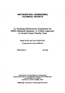
The table shows the timings in seconds for the brute force method and our new hierarchical method. We used a threshold (difference in BRDF values) of 0.001 for the hierarchical method, which yields the same visual quality as the brute force method, see Figure 4 (color plates). We have also tested different sizes of environment maps. The results indicate that the brute force method has linear complexity in the number of touched pixels, whereas our hierarchical method is sublinear. 5.2 Hardware accelerated Prefiltering For interactive applications it would be interesting if environment map prefiltering could be done on the fly, for example using graphics hardware. This means that if the scene changes, glossy reflections change accordingly. In this paper, we will only deal with the accelerated filtering of a given environment map. It has been shown in [19] that environment maps can be generated on the fly. Live video capturing of an environment map is also conceivable. For example the Omnicam [16] directly captures an environment as parabolic map. As seen in the previous section, environment map prefiltering always uses a two dimensional filter kernel, which is shift-variant in general, but depends on the representation of the environment map. The OpenGL imaging subset only supports shiftinvariant two dimensional filters of certain sizes [17]. Hence, for hardware accelerated prefiltering we have to choose an environment map technique that uses only two dimensional environment maps with a BRDF which results in a shift-invariant filter over the hemisphere, and an environment map representation that keeps the filter shift-invariant. The Phong model has a shift-invariant filter kernel over the hemisphere, since its cosine lobe is constant for all reflected viewing directions ~rv . It is also radially symmetric about ~rv . The filter size can also be decreased if smaller BRDF values are clamped to zero (will be necessary due to the restricted filter size of the graphics hardware). The filter shape is obviously circular, since it is radially symmetric. Therefore Phong environment maps fulfill the necessary requirements for hardware accelerated prefiltering. We still need to find an environment map representation that maps the shift-invariant circular filter kernel from the hemisphere to a shift-invariant circular filter kernel in texture space. It turns out that the dual paraboloid mapping proposed by Heidrich and Seidel [10] comes close to this desired property. A circular filter kernel which is mapped from the parabolic environment map back to the hemisphere is also (almost) circular. A distortion occurs depending on the radius and the position of the filter. To visualize the distortion, we project a circular filter kernel with a radius of r (r = 1 is half the width of the parabolic map) from the parabolic map back to the sphere and measure the error; see right side of Figure 3. We measure how much the distances from the center of the 8

d: distance from center of paraboloid to center of filter kernel

25% 20%

r: radius of filter kernel

15% 10%

filter kernel

5%

dual paraboloid environment map

0% 0.4 r

0.2 0

0

0.2

0.4

0.6

1

0.8 d

Fig. 3. Distortion of a circle when projected from a paraboloid map back to the sphere.

projected circle to its border deviate from a constant radius. The maximum deviation is used as the error, shown on the left side of the same figure. The distortion depends on the radius of the filter kernel and also on the distance d of the filter’s center from the parabolic map’s center (i.e. the center of the front- or backfacing paraboloid). The distortion goes up to 25% for large radii, but in these cases the prefiltered environment map will be very blurry, so that the distortion will not lead to visible errors. For smaller radii the distortion remains fairly small and again no visible artefacts occur. Although the shape of the filter almost remains the same in the parabolic space, the radius of the filter kernel varies with the distance d. The ratio between the smallest filter radius and largest filter radius is about 2. We will overcome this problem by generating two prefiltered environment maps, one with the smallest (yields map S) and one with the largest necessary filter size (yields map L). Then we blend between both prefiltered environment maps. The value with which we need to blend between both maps is different for different pixels in the parabolic environment map, but it depends only on the distance d and is always d2 . For a pixel in the center of the paraboloid this means that we use 0% of map L and a 100% of map S; for a pixel with distance d = 0.5 to the center of the parabolic map, we use 25% of map L and 75% of map S, and so on. Algorithm. The actual algorithm is fairly simple. First we create a mip-map of the parabolic environment map, then we load the environment map (plus the mip-map) into texture memory. The user has to specify the Phong exponent to be used and a limit when BRDF values from the Phong model can be clamped to zero, which is used to restrict the kernel size in the first place. Then we compute the two necessary filter radii, r s for the small filter and rl for the large filter. If a kernel size is larger then the maximum supported OpenGL kernel size, we scale the environment map and the filter by 0.5 until it is within the supported kernel size. Now we get to the actual filtering part: 1. Set the camera to an orthographic projection (so that we can draw the environment map seen from the top). 2. Draw alpha texture with d2 to alpha channel 3. For both radii rs and rl : 4. While rs (resp. rl ) < hardware supported filter size: 5. Divide rs (resp. rl ) by 2. Double the shrink factor. 6. Draw environment map shrunk by the shrink factor (uses mip-mapping). 7. Sample Phong model into the filter. 8. Filter the environment map with it (OpenGL convolution). 9

9. 10. 11. 12. 13. 14.

Store it again as texture map (RGBα texture). Draw environment map S. Blend environment map L with it (using d2 ). Store again as a texture map. Set up real camera. Draw reflective object with generated environment map.

One problem arises when the center of the filter kernel is close to the border of the environment map. Part of the filter kernel will be outside the actual environment map, thus including values from outside the environment map. This can be solved by including a large border in the environment map. It should also be mentioned, that the graphics hardware clamps all numbers to the [0, 1] range, and therefore the original environment map cannot have a high dynamic range. Results. We have tested our algorithm on an SGI O2 where it achieves interactive rates. All the tests were done with parabolic environment maps with 512 × 1024 pixels. The border was 64 pixels in each direction (for each face). The maximum kernel size we used was 7 (larger kernel sizes considerably degrade the convolution speed on an O2). We measured the following timings (reflective sphere, 2592 triangles): exponent 10 50 100 250 500

filter size small large 174 260 78 136 56 100 36 66 26 48

shrink factor small large 32 64 16 32 8 16 8 16 4 8

fps 2-pass

fps 1-pass

25 20 16 16 9

33 33 25 25 11

Please note that filtering was performed for every frame, even though the Phong exponent did not change. We have included timings for the two-pass convolution (i.e. using the small and the large filter) and for a one-pass convolution (using only the small filter). Furthermore we have included the filter sizes in pixels that would have been required (the BRDF clamp value was set to 0.1) and the necessary shrink factor to get filter sizes within a maximum size of 7 pixels. You can see that for small Phong exponents hardware prefiltering is very interactive. For larger Phong exponents the rendering speed is slower, because filtering cannot be done with a shrunk environment map. For a visual comparison please see Figure 4 (color plates). You can see that the hardware method generates dark borders, which does not pose a problem since these are not used for rendering. Figure 5 shows renderings with different environment maps and different Phong exponents; they all run at interactive rates. It should be mentioned that the two dimensional approximation to an isotropic BRDF proposed by Kautz and McCool [11] can also be used, since it also fulfills the necessary requirements (see beginning of this section). Hence their approximation can be used to prefilter environment maps with arbitrary isotropic BRDFs in real-time. 5.3 Anisotropic Environment Maps So far, there has not been an environment map technique that can also be applied to anisotropic BRDF models. Generally, an anisotropic BRDF depends on many parameters, which then results in a five dimensional environment map, see Section 4. 10

We need to look for a model which allows to create a lower dimensional environment map. The Banks model [1], which is simple and depends only on dot products, yields a three dimensional environment map if self shadowing is excluded. The BRDF is given by: q  q 1 2 2 ~ ~ ~ 1− < l, ~t > 1− < ~v , ~t > − < l, ~t >< ~v , ~t > −s fr (~v , l) := , (1 − s)2 where we have extended the original Banks model with a new parameter s ∈ [0, 1), which allows to have sharper highlights. The environment map equation becomes:  Z q q 1− < ~l, ~t >2 1− < ~v , ~t >2 − < ~l, ~t >< ~v , ~t > −s Lbanks (x; ~v , ~n, ~t) = Ω

1 Li (x; ~l) < ~n, ~l > d~l. (1 − s)2 To decrease the dimensionality of this environment map, we discard the self-shadowing term < ~n, ~l >, and then reparameterization gives us the following three dimensional environment map:  Z q q 2 2 ~ ~ ~ ~ ~ ~ ~ ~ 1− < l, t > 1− < ~v , t > − < l, t >< ~v , t > −s Lbanks (x; t, < ~v , t >) = Ω

1 Li (x; ~l) d~l. (1 − s)2 Now we have an anisotropic prefiltered environment map. In order to render an object using this environment map it is necessary to compute the 3D texture coordinates at every vertex by hand, i.e. the two coordinates of the unit vector ~t and the third coordinate corresponding to < ~v , ~t >. This anisotropic environment map can then be rendered at interactive rates if the hardware supports three dimensional texturing. In Figure 6 we show a teapot with an anisotropic material, which was done with an anisotropic prefiltered environment. Since the self-shadowing term is omitted, an object using this environment map does reflect light from behind it. This is usually not noticeable unless a bright light source shines “through”.

6 Conclusions We have proposed a general notation of prefiltered environment maps, according to which we have classified previously proposed prefiltered environment map techniques. We have developed three new techniques. First, we have used a new hierarchical prefiltering method which is on average about 10 times faster than a brute force prefiltering method. Second, we have proposed a hardware accelerated prefiltering method, which can prefilter environment maps in real-time, if the used reflectance model translates to a constant and radially symmetric filter kernel. Third, we have proposed an anisotropic prefiltered environment map using the Banks model. Future research should investigate the possibility to use difference pyramids first introduced by Burt and Adelson [4] to further speed-up the hierarchical prefiltering. Anisotropic environment maps using a constant shaped anisotropic lobe (à la Phong) should be researched as a possible alternative to the Banks model. 11

7 Acknowledgements We would like to thank Jonas Jax and Jeff Heath who put their beautiful environment maps online. This work was partially supported by the SIMULGEN ESPRIT project #35772 and by the Universitat de Girona under grant BR98/I003.

References 1. BANKS , D. Illumination in Diverse Codimensions. In Proceedings SIGGRAPH (July 1994), pp. 327–334. 2. BASTOS , R., H OFF , K., W YNN , W., AND L ASTRA , A. Increased Photorealism for Interactive Architectural Walkthroughs. In 1999 ACM Symposium on Interactive 3D Graphics (April 1999), J. Hodgins and J. Foley, Eds., ACM SIGGRAPH, pp. 183–190. 3. B LINN , J., AND N EWELL , M. Texture and Reflection in Computer Generated Images. Communications of the ACM 19 (1976), 542–546. 4. B URT, P., AND A DELSON , E. A Multiresolution Spline with Application to Image Mosaics. ACM Transactions on Graphics 2, 4 (October 1983), 217–236. 5. C ABRAL , B., O LANO , M., AND N EMEC , P. Reflection Space Image Based Rendering. In Proceedings SIGGRAPH (August 1999), pp. 165–170. 6. D IEFENBACH , P., AND BADLER , N. Multi-Pass Pipeline Rendering: Realism For Dynamic Environments . In 1997 ACM Symposium on Interactive 3D Graphics (April 1997), M. Cohen and D. Zeltzer, Eds., ACM SIGGRAPH, pp. 59–70. 7. G REENE , N. Applications of World Projections. In Proceedings Graphics Interface (May 1986), pp. 108–114. 8. G REENE , N. Environment Mapping and Other Applications of World Projections. IEEE Computer Graphics & Applications 6, 11 (November 1986), 21–29. 9. H EIDRICH , W., AND S EIDEL , H. Realistic, Hardware-accelerated Shading and Lighting. In Proceedings SIGGRAPH (Aug. 1999), pp. 171–178. 10. H EIDRICH , W., AND S EIDEL , H.-P. View-Independent Environment Maps. In Eurographics/SIGGRAPH Workshop on Graphics Hardware (1998), pp. 39–45. 11. K AUTZ , J., AND M C C OOL , M. Approximation of Glossy Reflection with Prefiltered Environment Maps. In Proceedings Graphics Interface (May 2000), pp. 119–126. 12. K IRK , D., AND A RVO , J. Unbiased Sampling Techniques for Image Synthesis. In Proceedings SIGGRAPH (July 1991), pp. 153–156. 13. L ISCHINSKI , D., AND R APPOPORT, A. Image-Based Rendering for Non-Diffuse Synthetic Scenes. In Nineth Eurographics Workshop on Rendering (June 1998), Eurographics, pp. 301–314. 14. M ILLER , G., AND H OFFMAN , R. Illumination and Reflection Maps: Simulated Objects in Simulated and Real Environments. In SIGGRAPH ’84 Course Notes – Advanced Computer Graphics Animation (July 1984). 15. M ILLER , G., RUBIN , S., AND P ONCELEON , D. Lazy Decompression of Surface Light Fields for Precomputed Global Illumination. In Nineth Eurographics Workshop on Rendering (June 1998), Eurographics, pp. 281–292. 16. NAYAR , S. Catadioptric Omnidirectional Camera. In Proceedings of IEEE Conference on Computer Vision and Pattern Recognition (june 1997). 17. N EIDER , J., DAVIS , T., AND W OO , M. OpenGL - Programming Guide. Addison-Wesley, 1993. 18. P HONG , B.-T. Illumination for Computer Generated Pictures. Communications of the ACM 18, 6 (June 1975), 311–317. 19. SGI. Iris performer. http://www.sgi.com/software/performer/brew/envmap.html. 20. S TÜRZLINGER , W., AND BASTOS , R. Interactive Rendering of Globally Illuminated Glossy Scenes. In Eighth Eurographics Workshop on Rendering (June 1997), Eurographics, pp. 93– 102.

12

Unfiltered original

Classic

Hierarchical

Hardware 2−pass

Hardware 1−pass

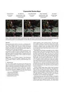
Fig. 4. Comparison of the different filtering methods. Filtering was done with the Phong model and an exponent of 100. From left to right: Unfiltered, the classic method, our new hierarchical method, the hardware accelerated method with two and one pass(es). The original environment map is 128 × 256 pixels in size with a border of 16 pixels.

N = 50. 20 Hz.

N = 500. 9 Hz.

N = 50. 20 Hz.

N = 500. 9 Hz.

Fig. 5. Two scenes rendered with a glossy reflective torus (SGI O2). Filtering is done with the Phong model (exponent of 50 and 500) for every frame, but interactive rates are still achieved. The original environment maps are 512 × 1024 pixels in size with a border of 64 pixels.

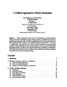
Fig. 6. The two images on the left, show a teapot with an anisotropic environment map using the Banks model (s = 0.99). The images on the right show slices of the three dimensional environment map (for ^(~v , ~t) = 44◦ , 39◦ , 35◦ ).

13