A Unified Apriori-like Algorithm for Conjunctive Query Containment Fang Wei
Georg Lausen
University of Freiburg
University of Freiburg
[email protected]
[email protected]
ABSTRACT The design of containment checking algorithms for conjunctive queries with arithmetic comparisons and safe negations (CQ¬6= s) is fundamental to many database applications. However, it is a challenging task due to the intractability of the problem. Existing algorithms are either computationally too expensive, or capable to deal with only a fragment of these extensions. In this paper we propose a novel algorithm for testing containment of CQ¬6= s. The key idea of the algorithm is to recursively consider only the containment mappings between the positive subgoals of the queries, instead of testing all the symbol mappings. Thus the number of test cases can be drastically reduced. Our algorithm enables further an on the fly execution of the normalization step. With the observation that the property of anti-monotonicity holds in our problem setting, we develop an Apriori-like algorithm as a sub-function of the containment checking algorithm, to which desirable pruning strategies are applied. Furthermore, we identify the criteria to reduce the number of test sets, and demonstrate that two additional improvements to the containment checking algorithm: node clustering and tuple pruning can further speed up the checking process.
1.
INTRODUCTION
Conjunctive query (CQ) containment checking is a classical problem in database research. Besides the traditional role it plays in semantic optimization, query containment has been shown crucial in data integration [9], data exchange [6], and semantic web [14], just to mention a few. Since it has been proved that the containment checking problem of CQs is NP-complete [5], many research works have been focused on extracting fragments of CQ for which the containment checking is tractable. Specifically, it has been shown that if the containing query is acyclic, then a linear time algorithm can be obtained for the containment checking [21]. Moreover, if each database predicate does not occur more than twice in the body of the contained query, the containment checking is tractable as well [16]. Recently,
Permission to make digital or hard copies of all or part of this work for personal or classroom use is granted without fee provided that copies are not made or distributed for profit or commercial advantage and that copies bear this notice and the full citation on the first page. To copy otherwise, to republish, to post on servers or to redistribute to lists, requires prior specific permission and/or a fee. IDEAS08 2008, September 10-12, Coimbra [Portugal] Editor: Bipin C. DESAI Copyright 2008 ACM 978-1-60558-188-0/08/09 ...$5.00.
Gottlob et al. [7] have proposed the concept of hypertree width, which is a generalization of acyclicity. If the containing query has bounded hypertree width, the containment checking can be performed in polynomial time. All of the above results, however, consider only the SPJ (selection, projection and join) queries. Often in real applications, users wish to query the database with arithmetic comparisons like salary > 10k, as well as with some safe negations (not exists in SQL). We denote such extensions of the CQ as conjunctive query with arithmetic comparisons (CQ6= ), conjunctive query with safe negations (CQ¬ ), and conjunctive query containing both arithmetic comparisons and safe negations (CQ¬6= ). Containment checking for CQs with such extensions is harder. It has been proved that the complexity of containment checking for CQ6= s is Πp2 -complete [10, 19]. Furthermore, Kolaitis et al. have shown that even if the positive subgoals of the containing query constitute an acyclic hypergraph, the complexity remains Πp2 -hard [11]. Therefore, it is a challenging task to design practical containment checking algorithms for the CQs with these extensions. For CQ6= s, there does exist an elegant algorithm proposed ¨ by Zhang and Ozsoyoglu [22], as well as by Gupta et al. [8]. We denote this algorithm as ZOG algorithm. The ZOG algorithm first searches for all the containment mappings between the positive subgoals and then proceeds with an implication test of the arithmetic comparisons according to these containment mappings. However, it has been shown that in order to test the containment, both queries have to be first normalized. The normalization increases (1) the number of arithmetic comparisons, and (2) the number of containment mappings between the queries. Since the efficiency of the implication test depends on both factors, normalization is not desired. Afrati et al. [2] proposed several fragments of CQ6= s, where the normalization is not necessary. However, in general the normalization step cannot be avoided. For CQ¬ s, Wei and Lausen [20] proposed an algorithm which recursively tests the containment mappings of the positive subgoals. Based on this work, some algorithmic improvements were proposed using the concept of graph homomorphism [12]. However, neither of these methods can deal with arithmetic comparisons. To the best of our knowledge, the only existing algorithm checking containment of CQ¬6= s is from Levy and Sagiv [13] (see also the description given by Ullmann [18]). We denote this algorithm as LSU algorithm. The LSU algorithm follows the two consecutive steps: (1) exhaustively generate all the canonical databases of the contained query, and (2) apply the containing query on these canonical databases. Since the number of canonical databases is finite, the containment
test always terminates. Unfortunately, this algorithm is not viable in practice, even for queries with relatively small size. For illustration consider the conjunctive queries q1 and q2 in Example 1.1: Example 1.1. q1 : ans() q2 : ans()
← p(X, Y, Z), p(Z, U, V ), ¬p(U, Y, V ). ← p(A, B, C), p(D, E, F ), B 6= F, D 6= E.
According to LSU algorithm, if we only consider one partition: {p(0, 1, 2), p(2, 3, 4)}, then there exist 53 tuples with the form p(·, ·, ·) over the domain {0, 1, 2, 3, 4}. Hence the 3 number of all possible canonical databases sums up to 25 = 125 2 , which is computationally too expensive. Furthermore, it is unclear, how the partitioning of the canonical databases should be done, if the CQ¬6= query contains arithmetic comparisons with constants (such as X < 5).
1.1 Our Contributions Despite numerous theoretical results, several problems concerning the containment checking of CQ¬6= s are still open: 1. Is it possible to improve the LSU algorithm to obtain an acceptable running time? 2. Could the ZOG algorithm be further improved, so that the normalization step is only executed when necessary? 3. Does a feasible algorithm exist, which can deal with any kind of arithmetic comparisons and safe negation in a uniform way? In this paper, we propose a novel algorithm for testing containment of CQ¬6= s, which positively answers all these questions. The key observation is as follows: Consider two CQ¬6= s q1 and q2 . q1 ⊑ q2 is to be checked. The ultimate goal of our algorithm is finding a more specific query q of q1 , such that there exists a canonical database D of q, and q2 (D) = False. If such a query q exists, we conclude with q1 6⊑ q2 , otherwise q1 ⊑ q2 holds. Therefore, we are interested in the following question: How to generate all these more specific queries of q1 efficiently? We prove that it suffices to systematically extend q1 by adding the subgoals (or arithmetic comparisons) with the form ρi (co(cnj )) to q1 , where ρi is the containment mapping from positive subgoals of q2 to those of q1 , cnj is either a negated subgoal or an arithmetic comparison in the body of q2 , and co(cnj ) is the complement (see Definition 2.4) of cnj . This way, (1) we can deal with both arithmetic comparisons and safe negations in a uniform way, and (2) the number of tests can be drastically reduced, comparing with the method of generating all the symbol mappings between two queries. Example 1.2. q1 : ans() q2 : ans()
← p(X, Y ), ¬p(Y, X). ← p(A, B), A 6= B.
Consider Example 1.2, we first decide the containment mappings of the positive subgoals of q2 to those of q1 , which is ρ : A → X, B → Y . Then we generate a more specific query of q1 by adding ρ(co(A 6= B)) (which turns out to be X = Y ) into q1 . Now the more specific query q has the form q : ans()
← p(X, Y ), ¬p(Y, X), X = Y.
It is obvious that q is unsatisfiable, because it is equivalent to the query q ′ : ans()
← p(X, Y ), ¬p(Y, X), X = Y, p(X, X), ¬p(X, X).
which contains contradictory subgoals p(X, X) and ¬p(X, X). This observation inspires our definition of the complete form of the queries (see Definition 2.14), where additional subgoals resulting from the introduced variable equivalence (such like X = Y ) have to be added. The concept of complete form of queries not only serves for the syntactic testing of unsatisfiability (as in Example 1.2), but also, which is more important, ensures the existence of a canonical database of the query, which enables an inverse containment mapping from the database to the positive subgoals in the query. This property is crucial for proving the main theorem (Theorem 3.1). The rewriting of a query into its complete form, however, could result in new containment mappings between the positive counterpart of the queries. In such cases, we have to generate the new containment mappings and execute the process recursively. It should be pointed out that the generation of the complete form is, to some extent, the reminiscence of the normalization step of the ZOG algorithm. However, our method differs from the normalization significantly in that the generation of the complete form is done on the fly, i.e., it is created only if necessary. On the contrary, the normalization step of the ZOG algorithm is executed before any containment test starts. It turns out that the algorithm directly interpreted from the theorem is not optimal. Given a fixed set of containment mappings, an exponential number of more specific queries of q1 have to be generated and tested. We observe that the so-called anti-monotonicity property holds in our problem setting. That is, if a query q is unsatisfiable, then any other specific query extended from q (i.e., by adding subgoals or arithmetic comparisons into the body of it) is unsatisfiable as well. Thus any further extension of this query can be avoided. It is well known that with the anti-monotonicity property, the Apriori-like algorithm can be applied. Based on this observation, we construct a level-wise Apriori algorithm, where effective pruning strategies can be applied. Moreover, we prove the early termination condition, i.e., during the level wise generation of test cases, if some unsatisfiable condition is fulfilled, the algorithm stops and returns the result. Moreover, after identifying the criteria to reduce the number of test sets, we propose two additional improvements, namely node clustering and tuple pruning, for the Apriori algorithm. We demonstrate that by integrating these strategies into our containment checking algorithm, significant reduction on both time and space consumption can be achieved. Of course, since it is proved that the containment of only CQ6= s is already Πp2 -complete, no tractable algorithm for our problem can be obtained unless P=NP. In this paper we do not continue research to find tractable fragments of the problem; instead we concentrate on the general case and develop algorithms for which we can expect reasonable performance which make them useful in practical cases. This situation is akin to mining frequent item sets, a problem computationally intractable in general, however in practice still managebale because of the clever design of so-called Apriori algorithms [3]. The rest of the paper is organized as follows. Section 2 introduces the definitions of CQ¬6= , query evaluation, query
containment and satisfiability. We state the main theorem (Theorem 3.1) and give the proof in Section 3.1. In Section 3.2 the basic algorithm Containment is introduced, which is followed by the correctness and completeness proof of the algorithm w.r.t. Theorem 3.1. In Section 3.3 we propose the Apriori algorithm as a sub-function for Containment, where important pruning strategies are applied. Further in Section 4 we propose two improvements for the Apriori algorithm, node clustering and tuple pruning. The conclusions are given in Section 5.
2.
PRELIMINARIES A (boolean)
1
conjunctive query (CQ) q is of the form ans()
← p1 , . . . , p n .
¯i ) where each pi (1 ≤ i ≤ n) is a subgoal of the form gi (X ¯i is either a variable or a and every predicate argument in X constant. We denote all the variables in q as vars(q) and all the constants as cons(q). Definition 2.1 (CQ¬6= , CQ6= and CQ¬ ). A conjunctive query with arithmetic comparison and safe negation (CQ¬6= ) is of the form ans()
←
p1 , . . . , pn , cn1 , . . . , cnm .
where for some r with 1 ≤ r ≤ m, • cni (1 ≤ i ≤ r) has the form XθY or Xθa, where θ ∈ {, ≥, 6=, =}, X, Y are variables and a is a constant. • cni (r + 1 ≤ i ≤ m) has the form ¬hi (Y¯i ), where each argument in Y¯i is either a variable or a constant. We denote p1 , . . . , pn as q + , cn1 , . . . , cnm as q cn , cn1 , . . . , cnr as q c , and cnr+1 , . . . , cnm as q n . We assume all the CQ¬6= queries are safe, i.e., each variable in cn1 , . . . , cnm occurs in vars(q + ). If a conjunctive query contains only arithmetic comparisons, it is a CQ6= ; and if it contains only negated subgoals, it is a CQ¬ .
2.1 Known Framework Given a database D, we denote the active domain of D as adom(D). Definition 2.2 (Symbol mapping). Let q, q1 and q2 be CQ¬6= s, and D a database. • A symbol mapping from q to D is a mapping that maps every constant in cons(q) to the same constant and every variable in vars(q) to an element in adom(D). • A symbol mapping from q2 to q1 is a mapping that maps every constant in cons(q2 ) to the same constant in cons(q1 ) and every variable in vars(q2 ) to either a variable in vars(q1 ) or a constant in cons(q1 ). Definition 2.3 (Containment mapping). Let q, q1 and q2 be CQ¬6= s, and D a database. • A containment mapping ρ from q + to D is a symbol mapping from q + to D, such that for each pi ∈ q + , ρ(pi ) ∈ D holds. We denote all the containment mappings from q + to D as CMs(q + , D). 1
We consider in this paper only boolean queries.
• A containment mapping ρ from q2 + to q1 + is a symbol mapping from q2 + to q1 + , such that for each pi ∈ q2 + , ρ(pi ) ∈ q1 + . We denote all the containment mappings from q2 + to q1 + as CMs(q2 + , q1 + ).
2.1.1 Query Evaluation Given a database D and a conjunctive query q, we use q(D) = True to denote that q is evaluated True over D. It is well known that if q is a CQ, then q(D) = True if there exists a containment mapping from q to D [1]. On the contrary, q(D) = False if such a containment mapping does not exist. Before we are able to define the query evaluation for CQ¬6= s, we have to introduce first the complement operation. Roughly speaking, the complement of a negated subgoal is its positive counterpart, and the complement of an arithmetic comparison expression is the corresponding expression with the complement operation. Definition 2.4 (Complement). Let q be a CQ¬6= and cni be either an arithmetic comparison in q , or a negated subgoal. The complement of cni , denoted as co(cni ) is defined as follows: • If cni is an arithmetic comparison with the form XθY or Xθa, the complement of cni is an arithmetic com¯ or X θa ¯ where θ¯ is the comparison with the form X θY plement operation of θ. • If cni is a negated subgoal of the form ¬hi (Y¯i ), the complement of cni is the non-negated subgoal hi (Y¯i ). For instance, co(X 6= a) is X = a and co(¬g(X, Y )) is g(X, Y ). Definition 2.5 (Query evaluation of CQ¬6= ). Let D be a database and q a CQ¬6= of the form ans()
←
p1 , . . . , pn , cn1 , . . . , cnm .
where for some r ≤ m, every cni (1 ≤ i ≤ r) is an arithmetic comparison and every cni (r + 1 ≤ i ≤ m) is a negated subgoal. q(D) = True if and only if there exists a containment mapping ρ from q + to D, such that for every cni(1≤i≤r) , ρ(cni ) is True, and for every cni(r+1≤i≤m) , ρ(co(cni )) ∈ / D. q(D) = False if and only if for every containment mapping ρ ∈ CMs(q + , D), there exists a cni(1≤i≤r) , such that ρ(co(cni )) is True, or there exists a cni(r+1≤i≤m) , such that ρ(co(cni )) ∈ D.
2.1.2 Containment Checking Let q1 and q2 be conjunctive queries. q1 is contained in q2 , denoted as q1 ⊑ q2 , if and only if for every database D, such that q1 (D) is True, q2 (D) is True. Let q1 and q2 be CQs. q1 ⊑ q2 if and only if there is a containment mapping from q2 to q1 . Considering CQ6= s, a single containment mapping does not suffice. Instead, we need to check a set of containment mappings. Definition 2.6 (Normalization). [22] A CQ6= q is normalized if every variable occurs only once in q + and there does not exist any constant in q + . Any CQ6= query can be transformed into an equivalent normalized query as follows: (1) For all occurrences of a
Symbol CQ CQ6= CQ¬ CQ¬6= q+ q cn qc qn CMs(q2 + , q1 + ) CMs(q + , D)
Table 1: Symbols used in the paper Meaning Conjunctive query CQ with arithmetic comparison CQ with safe negation CQ with arithmetic comparison and safe negation ordinary positive subgoals of a CQ¬6= q arithmetic comparisons and negated subgoals of a CQ¬6= q arithmetic comparisons of a CQ¬6= q negated subgoals of a CQ¬6= q all the containment mappings from q2 + to q1 + all the containment mappings from q + to D
shared variable X in q + except the first occurrence, replace the occurrence of X by a new distinct variable Xi , and add X = Xi to q c ; (2) For each constant c in the query, replace the constant by a new distinct variable Z, and add Z = c to qc . Theorem 2.7. [22] Let q1 and q2 be the normalized CQ6= s. Let ρ1 , . . . , ρl be CMs(q2 + , q1 + ). Then q1 ⊑ q2 if and only if q1 c ⇒ ρ1 (q2 c ) ∨ . . . ∨ ρl (q2 c ). In the rest of the paper, we distinguish the containment (⊑) from the syntactical containment (⊆). We denote ⊆ as a pure subset relation of the queries, i.e., q1 ⊆ q2 means every element in q1 exists in q2 . The following trivial relationship holds: Lemma 2.8. Let q1 and q2 be CQ¬6= s as follows: q1 : ans() q2 : ans()
← q1 + , q1 cn . ← q2 + , q2 cn .
where q2 + ⊆ q1 + and q2 cn ⊆ q1 cn . Then q1 ⊑ q2 .
2.2 Extensions of Formalisms for CQ¬6= s 2.2.1 Satisfiability and Compact Normal Form It is well known that all CQs are satisfiable. It can be easily shown that CQ6= is satisfiable if the conjunction of its arithmetic comparisons is satisfiable. For CQ¬ s, the following holds: Corollary 2.9 (Folklore). A CQ¬ is satisfiable iff ¯ such that g(X) ¯ ∈ q+ there does not exist a subgoal g(X), n ¯ and ¬g(X) ∈ q . However, satisfiability of a CQ¬6= can not be tested according to the syntax of the query. For instance, let q be the query shown in Introduction: q : ans()
← p(X, Y ), ¬p(Y, X), X = Y.
It is obvious that q is unsatisfiable although both subqueries ans() ← p(X, Y ), ¬p(Y, X). and ans() ← p(X, Y ), X = Y. are satisfiable. To overcome this problem, we introduce the concept of the compact normal form. Definition 2.10 (Compact Normal Form). A CQ¬6= q is in compact normal form if the arithmetic comparisons of q do not imply any equality with the form X = Y or X = a.
Any CQ¬6= can be transformed into its compact normal form as follows: (1) We first partition the variables and constants in q into n disjoint subsets (equivalence classes) based on their equivalence relations. Note that there is at most one constant in each class. (2) For all the elements in each equivalence class, choose one representative Xi (i.e., if the class contains a constant a, then Xi = a; otherwise Xi is assigned with one arbitrary variable). (3) Rewrite each subgoal and each arithmetic comparison by replacing every variable with its representative. Note that all the compact normal forms of a give query q are equivalent upon isomorphism. The intuition behind the compact normal form is as follows: if a CQ¬6= is in compact normal form, then there is a total order of all variables so that a canonical database can be constructed by mapping each variable to a distinct constant. Proposition 2.11. Let q be a CQ¬6= in compact normal form as follows: ans()
←
p1 , . . . , pn , cn1 , . . . , cnm .
where for some r ≤ m, every cni (1 ≤ i ≤ r) is an arithmetic comparison and every cni (r + 1 ≤ i ≤ m) is a negated subgoal. Then q is satisfiable if and only if 1. the conjunction of cn1 , . . . , cnr is satisfiable, and ¯i ), such that gi (X ¯i ) ∈ 2. there does not exist a subgoal gi (X ¯i ) ∈ {cnr+1 , . . . , cnm } {p1 , . . . , pn } and ¬gi (X Proof. Since q is in compact normal form, it does not imply any equality with the form X = Y or X = a, then according to the arithmetic comparisons cn1 , . . . , cnr , we can construct a canonical database D as follows: generate a symbol mapping ρ that maps each constants in cons(q + ) into the same constant and each variable in vars(q + ) into a distinct new constant, such that ρ(vars(q + )) ∪ ρ(cons(q + )) are in total order. Let adom(D) = ρ(vars(q + )) ∪ ρ(cons(q + )), and ρ(q + ) be the canonical database D. Note that ρ is a oneto-one mapping and for every tuple t ∈ D, ρ−1 (t) ∈ q + holds. Since the conjunction of cn1 , . . . , cnr is satisfiable, then ρ(cni )(1≤i≤r) = True holds. It remains to show that for every i(r+1≤i≤m) , ρ(co(cni )) ∈ / D. Suppose on the contrary there is one cni(r+1≤i≤m) , such that ρ(co(cni )) ∈ D. Because ρ is a one-to-one mapping, ρ−1 (ρ(co(cni ))) ∈ q + holds, which implies that co(cni ) ∈ q + . This constructs a contradiction to the condition (2). Since we have shown that q(D) = True, q is thus satisfiable.
2.2.2 Core and Complete Form The concept of the compact normal form introduced in Section 2.2.1 is crucial to the satisfiability test of CQ¬6= s. Moreover, we have shown that if a query is in compact normal form, a canonical database can be constructed by mapping the variables into distinct constants. This is an important property in that it enables a inverse containment mapping from the canonical database into the positive subgoals of the query. However, given a query q, it is often desirable to obtain an equivalent query of q, without removing the subgoals, while preserving the property of compact normal form. For this purpose, we introduce the concept of core and complete form. Definition 2.12 (Core). Let q be a CQ¬6= , and q ′ a compact normal form of q. All the subgoals (both positive and negated) of q ′ is the core of q. It should be pointed out that the definition of core here differs from the concept of core in the data exchange context. The query in compact normal form (i.e., containing only a core as subgoals) need not to be minimal in terms of the size of the subgoals. For instance, consider the following CQ6= : Example 2.13. q : ans() ← p(X, Y ), p(X, X), X < 5. Query q is not minimal, since the subgoal p(X, Y ) is superfluous. However, it is in compact normal form, since X = Y is not implied. Thus {p(X, Y ), p(X, X)} is a core of q. Definition 2.14 (Complete form). A CQ¬6= q is complete if it contains a core of q. The transformation from a query into its complete form is straightforward. We first reduce the query q into its compact normal form q ′ , then add all the subgoals of q ′ into q. Proposition 2.15. Let q be a CQ¬6= , and q ′ is a complete form of q. q ≡ q ′ holds. Proof. Since q ⊆ q ′ , q ′ ⊑ q holds. It remains to prove that q ⊑ q ′ . Let D be any database s.t. q(D) = True, we show that q ′ (D) = True. Let ρ be the containment mapping from q + to D. Let p be a positive subgoal such that p = g(X1 , . . . , Xn ), if p ∈ q ′+ and p 6∈ q + , then g(X1 , . . . , Xn ) is a core subgoal. We have to show that ρ(g(X1 , . . . , Xn )) ∈ D. From the definition of compact normal form, p has a source subgoal g(Y1 , . . . , Yn ) in q + , s.t. Xi = Yi (1 ≤ i ≤ n) holds. We thus have ρ(g(Y1 , . . . , Yn )) ∈ D. Since ρ maps the equivalent variables into the same constant in D, we thus have ρ(g(X1 , . . . , Xn )) = ρ(g(Y1 , . . . , Yn )), therefore ρ(g(X1 , . . . , Xn )) ∈ D. Analogously, it is easy to show that for each negated core subgoal cn ∈ q ′ , ρ(cn) 6∈ D. We thus have shown that q ′ (D) = True.
3.
THEOREM AND ALGORITHMS FOR CONTAINMENT CHECKING
In this section, we concentrate on the containment checking problem on CQ¬6= s. Section 3.1 introduces the main theorem. In Section 3.2 we propose the basic algorithm Containment, which is followed by the sub-function Apriori discussed in Section 3.3.
3.1 Containment Theorem Theorem 3.1. Let q1 and q2 be CQ¬6= s as follows: q1 : ans() q2 : ans()
← q1 + , q1 cn . ← q2 + , q2 cn .
Then q1 6⊑ q2 if and only if there exist a set of symbol mappings ρ1 , . . . , ρn from q2 to q1 and a satisfiable, complete query q of the form q : ans()
← q + , q cn .
such that 1. q1 + ⊆ q + and q1 cn ⊆ q cn , 2. q2 cn = cn1 , . . . , cnm and {ρ1 (co(cnl1 )), . . . , ρn (co(cnln ))} ⊆ q + ∪ q cn where {l1 , . . . , ln } ⊆ {1, . . . , m}, and 3. CMs(q2 + , q + ) ⊆ {ρ1 , . . . , ρn } Proof. (1) ⇒: Assume that there exists a satisfiable, complete query q, we show that there exists a database D, such that q1 (D) is True and q2 (D) is False. Since q is complete, it contains a core. Let core+ (q) (core− (q), resp.) be all the positive (negated, resp.) subgoals occurring in the core of q. Since query q is satisfiable, we can derive a total order for the variables and constants in core+ (q). According to this total order, we freeze core+ (q) into a database D by replacing each variable in core+ (q) into a distinct constant, while each constant in core+ (q) remains the same. We denote the containment mapping from core+ (q) into D as τ . Note that the mapping τ is one-toone. Furthermore, for each negated subgoal cn ∈ core− (q), τ (co(cn)) ∈ / D, because q is satisfiable. Note that the source of τ contains only those variables occurring in the core of q. Next we extend τ to γ, where the source of γ contains all the variables in q + . Let X be a variable which occurs in q + , but does not occur in core+ (q), and Y be the representative variable (or constant) of X, which occurs in core+ (q). If Y → c ∈ τ , then add X → c into γ. We show that γ is a containment mapping from q + to D: for every subgoal g(X1 , . . . , Xn ) ∈ q + , there is a corresponding subgoal g(Y1 , . . . , Yn ) ∈ core+ (q), s.t. Xi = Yi(1≤i≤n) hold. Thus γ(g(X1 , . . . , Xn )) = τ (g(Y1 , . . . , Yn )) ∈ D. We have shown that γ is a containment mapping from q + to D. Analogously, it can be easily proved that for every cn ∈ q cn , γ(co(cn)) ∈ / D. Hence we can conclude that q(D) = True holds. Because q ⊑ q1 , we have q1 (D) = True. Now we prove that q2 (D) = False. Let ρ be any containment mapping from q2 + to D. Since τ is a one-to-one mapping, ρ ◦ τ −1 is a containment mapping from q2 + to q + . From condition (3) we know that ρ ∈ {ρ1 , . . . , ρn }, further due to condition (2), there exists a cn ∈ q2 cn , such that ρ ◦ τ −1 (co(cn)) ∈ q + ∪ q cn . From the construction of τ , we know that if cn is an arithmetic comparison, then ρ ◦ τ −1 ◦ τ (co(cn)) is True, thus ρ(co(cn)) is True. Otherwise, cn is a negated subgoal, then we have ρ◦τ −1 (co(cn)) ∈ q + , thus ρ◦τ −1 ◦τ (co(cn)) ∈ D, then we have ρ(co(cn)) ∈ D. Therefore we can conclude that q2 (D) is False. (2) ⇐: We show that if q1 6⊑ q2 , then there exists a query q, that fulfills all the conditions in Theorem 3.1. Let D be a database, such that q1 (D) = True, and q2 (D) = False, q can be constructed incrementally as follows: Let γ be the containment mappings from q1 + to D, s.t. q1 (D) is True, and µ1 , . . . , µk be all the containment mappings from q2 +
to q1 + . We start from µ1 . Clearly, µ1 ◦ γ is a containment mapping from q2 + to D. Since q2 (D) is False, there are two possibilities: (1) there exists an arithmetic comparison cn ∈ q2 cn , such that µ1 ◦ γ(co(cn)) is True, or (2) there exists a negated subgoal cn ∈ q2 cn , such that µ1 ◦γ(co(cn)) ∈ D. For any of the two cases, we can add µ1 (co(cn)) into the body of q1 . Let this new query be q1 ′ . Clearly, q1 ′ is still satisfiable. Furthermore, it holds that γ is still the containment mapping from q1 ′ to D, such that q1 ′ (D) = True. After proceeding the procedure k times, we obtain a new satisfiable query as follows: q1 ′ : ans()
← q1 + , q1 cn , µ1 (co(cnl1 )), . . . , µk (co(cnlk )).
Note that q1 ′ contains new non-negated subgoals and arithmetic comparisons, but no new variable is introduced. If q1 ′ is not complete, then we transform it into complete form. We denote this new complete query as q1 ′′ . From Proposition 2.15 we know that q1 ′′ is satisfiable as well, and more importantly, it still holds that γ is the containment mapping from q1 ′′ to D, such that q1 ′′ (D) = True. Because of the introduction of new non-negated subgoals, it is possible that new containment mappings from q2 + to + q1 ′′ appear. If there is no new mapping introduced, we stop and q1 ′′ is the required query. Otherwise, we repeat the same procedure. Since there are finite numbers of variables in q1 and q2 , and during the process no new variables are introduced, hence the number of the containment mappings can not exceed the number of symbol mappings from q2 to q1 , which is finite. Therefore the process either halts after q is found, or reaches the fixpoint, which has the following form: q : ans()
←
q1 + , q1 cn , µ1 (co(cnl1 )), . . . , µm (co(cnlm )).
where µ1 , . . . , µm are all the symbol mappings from q2 to q1 . Hence q is satisfiable and fulfills all the conditions in Theorem 3.1. From Theorem 3.1 a Πp2 upper bound for containment checking of CQ¬6= queries can be easily obtained as follows: (1) guess a set of symbol mappings ρ1 , . . . , ρn from q2 to q1 , and a set of cnl1 , . . . , cnln from q2 cn ; (2) then construct the query q and transform it into complete form; (3) check whether all the containment mappings from q2 + to q + are in ρ1 , . . . , ρn . Since step (3) is an NP oracle, the Πp2 upper bound is obvious. However, the number of possible sets of symbol mappings is prohibitively large (double exponential), a naive guess-and-test algorithm does not have any practical use.
3.2 The Containment Algorithm Inspired from the ⇐ proof of Theorem 3.1, we need only to recursively check those containment mappings from q2 + to q1 + , instead of checking all the symbol mappings from q2 to q1 . Assume there are n containment mappings from q2 + to q1 + , and there are m elements in q2 cn , then the number of all the extended queries is mn . In general n is much smaller than all the symbol mappings, thus the search space is reduced. The main algorithm Containment is given in Algorithm 1. It takes q1 , q2 and ρ1 , . . . , ρn as input parameters, where ρ1 , . . . , ρn are all the containment mappings from q2 + to q1 + . For the time being let us assume that the sub-function Apriori returns all the satisfiable queries that are extended from q1 by adding the subgoals or arithmetic comparisons with the form ρi (co(cnli )). The technical details concerning
pruning strategies for Apriori are discussed in the following section. If Apriori returns an emptyset, this means all the queries extended from q1 with ρ1 , . . . , ρn are unsatisfiable. Thus every possible query q which fulfills the conditions in Theorem 3.1 is unsatisfiable. Containment returns yes. Otherwise, we transform all the extended queries into their complete form (line 4). Among all these complete queries, if there is a satisfiable query q such that no new containment mapping from q2 + to q + is generated, the algorithm halts with the answer no. Otherwise, we continue the checking process with these extended queries, but with only the newly generated containment mappings considered. Since the number of symbol mappings is finite, the algorithm will finally reach the fixpoint and halt. Algorithm 1 Containment(q1 , q2 , ρ¯) Input: ρ¯ = ρ1 , . . . , ρn are all the containment mappings from q2 + to q1 + . Output: yes if q1 ⊑ q2 , no otherwise. 1: 2: 3: 4: 5: 6: 7: 8: 9: 10: 11: 12: 13: 14: 15: 16: 17:
if {q1′ , . . . , qk′ } = Apriori(q1 , q2 , ρ1 , . . . , ρn ) is ∅ then return yes end if Transform every qi′ into complete form for i = 1 to k do γ¯i = newmappings(qi′ , q2 , ρ¯) if γ¯i == ∅ then return no end if end for for i = 1 to k do ans = Containment(qi′ , q2 , γ¯i ) if ans == no then return no end if end for return yes
Before we come to the sub-function Apriori, we prove that the algorithm Containment is correct and complete. Theorem 3.2. Algorithm Containment is correct and complete. Proof. the correctness proof is trivial. In the following we prove the completeness. Let q1 and q2 be CQ¬6= s. Assume that there exists a set of symbol mappings {ρ1 , . . . , ρn } and a satisfiable and complete query q as in Theorem 3.1. We show that algorithm Containment returns no. Let ρ1 , . . . , ρr be all the containment mappings from q2 + to q1 + . Since q1 + ⊆ q + , we have {ρ1 , . . . , ρr } ⊆ CMs(q2 + , q + ), thus {ρ1 , . . . , ρr } ⊆ {ρ1 , . . . , ρn } holds. Then query q1 ′ can be constructed as follows: q1 ′ : ans() ← q1 , ρ1 (co(cnl1 )), . . . , ρr (co(cnlr )). where {ρ1 (co(cnl1 )), . . . , ρr (co(cnlr ))} ⊆ q. Since q1 ′ ⊆ q holds, q1 ′ is satisfiable. The sub-function Apriori (line 1) returns all the satisfiable queries extended from q1 with ρ1 , . . . , ρr . Thus q1 ′ must be in the return set of Apriori. We then transform q1 ′ into its complete form. Note that q1 ′ ⊆ q still holds. If no more new containment mappings + from q2 + to q1 ′ is generated, Containment algorithm returns no (line 8). Otherwise the function is recursively called with the new containment mappings. A sequence of
satisfiable queries is generated with the relationship: ′
q1 ⊆ q1 ⊆ . . . ⊆ q by adding consecutively positive subgoals or arithmetic comparisons with the form ρi (co(cnli )) where 1 ≤ i ≤ n. Since Containment deploys an exhaustive search, the fixpoint will be reached as soon as q (or a subset of it) is generated. Algorithm Containment thus returns no as well (line 14).
3.3 The Apriori Algorithm In Section 3.2 we have presented the basic part of the containment checking algorithm. Given the upper bound, which is decided by the queries, algorithm Containment could hardly be improved further. Now we consider the subfunction Apriori. Each time the algorithm Containment calls Apriori, a set of satisfiable queries extended from q1 is returned. Note that the number of queries is possibly exponential in the size of the number of containment mappings. Therefore the operation in Apriori is costly on both time and space, and it is crucial to explore the opportunities to optimize the Apriori algorithm. Note that although an exponential number of extensions are to be tested, only the satisfiable queries are returned, so we are interested in the question: how to detect those unsatisfiable queries as early as possible? Indeed, if a query q is unsatisfiable, then any extended queries by adding new subgoals into q is unsatisfiable as well. Thus any further extension of q can be pruned. We formulate this property with the following corollary: Corollary 3.3. Given two queries q1 and q2 as follows: q1 : ans() q2 : ans()
← q1 + , q1 cn . ← q2 + , q2 cn .
where q1 + ⊆ q2 + and q1 cn ⊆ q2 cn . If q1 is unsatisfiable, then q2 is unsatisfiable. The property of Corollary 3.3 is called anti-monotonicity, which is fundamental to designing the Apriori-like algorithm with desirable pruning strategies [3]. Simply stated, with the Apriori algorithm the query q1 is extended level wise. At each level i, the query is extended only if all the queries that are more general at level i−1 are satisfiable. Otherwise the query will not be further extended. Let q1 and q2 be CQ¬6= s and ρ1 , . . . , ρn be all the containment mappings and q2 cn = cn1 , . . . , cnm . The level wise algorithm Apriori (Algorithm 2) proceeds iteratively as follows: At level one, we generated n unary relations R1 (ρ1 ), . . . , Rn (ρn ). Each relation Ri contains m tuples with the form ρi (co(cnj ))(1 ≤ j ≤ m). We remove those tuples t where q1 ∧ t is unsatisfiable. In each subsequent iteration, at level i + 1 all the i + 1-ary tuples are generated from level i. For each i + 1-tuple t, if any i-ary projection of t does not exist in the relations at level i, t will be deleted. This is realized with the semi-join operation at line 16 to 22 in Algorithm 2. Early termination. During the iteration, if any relation R becomes empty, the algorithm halts and returns the empty set (line 11). This is easy to understand, because every possible tuple in the relation at the last level contains at least one tuple in R. At the last level of the iteration, we obtain a single relation in which every tuple t has the property that q1 ∧ t is satisfiable. These tuples are returned for further processing in Algorithm 1.
Algorithm 2 Apriori(q1 , q2 , ρ¯) Input: ρ¯ = ρ1 , . . . , ρn are the containment mappings from q2 + to q1 + , q2 cn = cn1 , . . . , cnm . Output: A set of satisfiable queries more specific than q1 V with the form q1 ∧ n i=1 ρi (co(cnli )) 1: Generate n one-column relations L1 = {R1 , . . . , Rn } where the attribute for Ri is ρi 2: for i = 1 to n do 3: for j = 1 to m do 4: Insert tuple ρi (co(cnj )) into Ri 5: end for 6: end for 7: k = 1 8: repeat 9: Delete every tuple t in relations of Lk where q1 ∧ t is unsatisfiable 10: if any k-column relation in Lk is empty then 11: return ∅ 12: end if 13: Generate all the k + 1-column relations Lk+1 by the natural-join of relations in Lk 14: for all relation R in Lk+1 do 15: for all relation R′ in Lk do 16: if Attr(R′ ) ⊆ Attr(R) then 17: R = R ⋉ R′ 18: end if 19: end for 20: end for 21: k =k+1 22: until k > n 23: Let Ln = {R} /* there is one table in Ln */ 24: Delete every tuple t in R where q1 ∧ t is unsatisfiable 25: Add q1 to every tuple in R 26: return R
We denote the relation at the last level as final relation and the tuples in the final relation as final tuples. To simplify the presentation, given a relation R generated in the algorithm Apriori and a tuple t in R, if the context is clear, we use the tuple t is satisfiable by meaning that the query q1 ∧ t is satisfiable. With the following Example 3.4, which is adapted from [2], we demonstrate the containment checking process following Containment and Apriori algorithms. Note that in [2] the authors used this example by showing that the normalization step of ZOG algorithm can not be avoided. We will illustrate that the normalization step is done here on the fly. Example 3.4. [2] Consider the following queries q1 and q2 : q1 : ans()
←
q2 : ans()
←
p(X, Y, 2, 1, U, U ), p(1, 2, X, Y, U, U ), p(1, 2, 2, 1, X, Y ). p(X, Y, Z, Z ′ , U, U ), X < Y, Z > Z ′ .
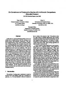
We check whether q1 ⊑ q2 . According to the algorithm Containment, we first generate all the containment mappings from q2 + to q1 + as follows: ρ1 : X → X, Y → Y, Z → 2, Z ′ → 1, U → U ρ2 : X → 1, Y → 2, Z → X, Z ′ → Y, U → U The Apriori algorithm is then called. At level 1, we generate two relations for ρ1 and ρ2 which are illustrated in Table 2 (a) and (b). In both relations, we remove the tuples which
result in unsatisfiability. Thus tuple 2 ≤ 1 and 1 ≥ 2 are removed. As a result, both relations contain one tuple. At level 2, all relations with two attributes are generated. In this case, one relation is generated, which is shown in Table 2 (c). Because both sub-relations of the tuple R3 exist at level 1, R3 succeeds the semi-join test. A new query q is returned from Apriori, with the arithmetic comparisons in R3 (X ≤ Y and X ≥ Y ) added: q:
← p(X, Y, 2, 1, U, U ), p(1, 2, X, Y, U, U ), p(1, 2, 2, 1, X, Y ), X ≤ Y, X ≥ Y.
ans()
Since q implies X = Y , we transform q into its complete form q ′ : q′ :
← p(X, Y, 2, 1, U, U ), p(1, 2, X, Y, U, U ), p(1, 2, 2, 1, X, Y ), X ≤ Y, X ≥ Y. p(X, X, 2, 1, U, U ), p(1, 2, X, X, U, U ), p(1, 2, 2, 1, X, X).
ans()
where the underlined subgoals are newly generated due to the equivalence X = Y . Three new containment mappings are thus generated: ρ3 : X → X, Y → X, Z → 2, Z ′ → 1, U → U ρ4 : X → 1, Y → 2, Z → X, Z ′ → X, U → U ρ5 : X → 1, Y → 2, Z → 2, Z ′ → 1, U → X and the Apriori procedure is called, however with newly generated containment mappings ρ3 , ρ4 and ρ5 . The same procedure is executed and three relations are generated at level 1. as illustrated in Table 2 (d), (e) and (f ). Since every tuple in R6 results in a unsatisfiable query, the early termination condition is fulfilled. Thus the Apriori sub-function returns ∅. The algorithm Containment finally returns yes.
Table 2: Relations generated for Example 3.4 (a) R1
(b) R2
ρ1 X≥Y 2≤1
ρ2 1≥2 X≤Y
(c) R3 ρ1 X≥Y
4.
ρ2 X≤Y
First call level 1
First call level 2
(d) R4
(e) R5
(f) R6
ρ3 X≥X 2≤1
ρ4 1≥2 X≤X
ρ5 1≥2 2≤1
Second call level 1
FURTHER IMPROVEMENTS
In this section, we propose two algorithms to further improve the time and space efficiency of the algorithm Apriori, with the following objectives: (1) minimization of the number of the final tuples, and (2) minimization of the intermediate tests in the level wise iteration. Section 4.1 considers the improvement of the algorithm in terms of task (2), and in Section 4.2 we propose further improvements concerning task (1).
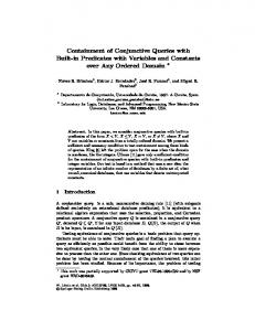
4.1 Node Clustering Although our algorithm makes use of the concept of the Apriori algorithm to process the satisfiability checking, it differs from the classical problem setting in that our algorithm returns only the final tuples at the last step Ln . The generation of the intermediate tuples can prevent the unsatisfiable tuples from further being extended at an early stage, but these intermediate tuples are not returned. Therefore if the number of the intermediate tuples can be reduced, the time and space consumption of the algorithm will be accordingly reduced. Assume that at level i of the Apriori algorithm, if several relations contain only one tuple, the conjunction of all these tuples will occur in every tuple of the final relation. Thus if all these tuples are clustered into one relation, many intermediate relations containing subsets of these tuples need not to be generated. We denote this operation as node clustering. Procedure 3 Node Clustering 1: Let R1 , . . . , Rr be all the single tuple relations in Lk 2: R = R1 ⊲⊳ . . . ⊲⊳ Rr 3: Let Rr+1 , . . . , Rm be all the relations such that Attr(Ri ) ∩ Attr(R) 6= ∅ where (r + 1 ≤ i ≤ m) 4: for i = r + 1 to m do 5: R = R ⋉ Ri 6: end for 7: remove R1 , . . . , Rm from Lk , add R into Lk 8: k = |R| We give a sketch of the node clustering algorithm in Procedure 3. This procedure can be inserted between the line 12 and 13 of the Apriori algorithm. Note that in the last line of Procedure 3, the level number k is increased to |R|, so that the intermediate relations between level |R| and k need not to be generated. We illustrate the node clustering operation with Example 4.1. Example 4.1. Consider the conjunctive queries q1 and q2 as follows: q1 : ans() q2 : ans()
← p(X, Y, Z), p(Z, U, V ), ¬p(X, Y, U ). ← p(A, B, C), p(D, E, F ), B 6= F, D 6= E.
The containment mappings from q2 + to q1 + are as follows: ρ1 ρ2 ρ3 ρ4
: A → X, B → Y, C → Z, D → Z, E → U, F → V : A → X, B → Y, C → Z, D → X, E → Y, F → Z : A → Z, B → U, C → V, D → Z, E → U, F → V : A → Z, B → U, C → V, D → X, E → Y, F → Z
The relations generated at level 1 are given in Table 3. After the satisfiability checking of the first level, the tuple Z = U is removed from R1 , R3 and R4 because q1 ∧ (Z = U ) is unsatisfiable. Now each of the relations R1 , R3 and R4 contains one tuple, as shown in (e), (g) and (h) of Table 3. We then cluster these relations into a new relation R5 , which is illustrated in (i) of Table 3. Since the correctness of the node clustering operation is straightforward, we omit the proof here.
4.2 Tuple Pruning When considering a tuple t in the final relation, we have so far made the assumption that the satisfiability of a tuple is independent from other tuples. In this section, we analyze
Table 3: Relations generated for Example 4.1. Relations (a),(b),(c),(d) are generated at level 1, with relations (e),(f ),(g),(h) after the deletion of the tuple Z = U , and the clustered relations (i),(j) after node clustering (a) R1
(b) R2
(c) R3
(d) R4
ρ1 Y =V Z=U
ρ2 Y =Z X=Y
ρ3 U =V Z=U
ρ4 Z=U X=Y
(e) R1
(f) R2
(g) R3
(h) R4
ρ1 Y =V
ρ2 Y =Z X=Y
ρ3 U =V
ρ4 X=Y
(i) R5 ρ1 Y =V
ρ3 U =V
(j) R2 ρ4 X=Y
ρ2 Y =Z X=Y
the inter-tuple relationship, and show that a tuple t can become redundant, due to the existence of another tuple t′ as its witness, although t itself is satisfiable. Let us consider a simple example. Assume that at level i, there is a tuple t containing X < 15, and at level i + 1, we extend t to t1 and t2 with the attribute ρ by adding ρ(co(cn1 )) and ρ(co(cn2 )) respectively. Assume ρ(co(cn1 )) = X < 16 and ρ(co(cn2 )) = X > 8. Clearly, t → X < 16 holds. This means, adding ρ(co(cn1 )) to t does not make t more specific (i.e., t1 is equivalent to t). We call t1 is a witness of t2 and consider t2 as a redundant tuple which can be removed, although t2 itself is satisfiable. We name such an operation as tuple pruning. The intuition behind tuple pruning is as follows: if at last a satisfiable query q is found, which contains t2 and fulfills all the conditions in Theorem 3.1, then we can prove that another query q ′ exists, by simply adding ρ(co(cn1 )) into q, such that q ′ fulfills the conditions in Theorem 3.1 as well. In Procedure 4 we give the sketch of the tuple pruning algorithm. This procedure can be inserted between line 12 and 13 of Algorithm 2, however before the procedure node clustering. Note that implication (→) in Procedure 4 can be defined as follows: let q be a CQ¬6= , ρ be some containment mapping and cn be either an arithmetic comparison or a negated subgoal, then q → ρ(co(cn)) means that q ∧ ρ(cn) is unsatisfiable. Procedure 4 Tuple Pruning Let R = (ρ1 , . . . , ρk ) be a k-ary relation in Lk if there is a tuple hρ1 (co(cnl1 )), . . . , ρk (co(cnlk ))i in R s.t. q1 , ρ1 (co(cnl1 )), . . ., ρi−1 (co(cnli−1 )), ρi+1 (co(cnli+1 )), . . ., ρk (co(cnlk )) → ρi (co(cnli )) then Delete the tuples in R with the form h ρ1 (co(cnl1 )), . . . , ρi−1 (co(cnli−1 )), ρi (co(cnlj )), ρi+1 (co(cnli+1 )), . . ., ρk (co(cnlk )) i where li 6= lj endif
Theorem 4.2. Procedure 4 is correct.
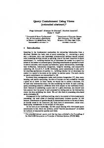
Proof. We show that during the iteration, if any tuple with the form t = hρ1 (co(cnl1 )), . . ., ρi−1 (co(cnli−1 )), ρi (co(cnlj )), ρi+1 (co(cnli+1 )), . . ., ρk (co(cnlk ))i is deleted according to Procedure 4, due to the existence of the witness tuple t′ = hρ1 (co(cnl1 )), . . ., ρi−1 (co(cnli−1 )), ρi (co(cnli )), ρi+1 (co(cnli+1 )), . . ., ρk (co(cnlk ))i, then if there is any satisfiable and complete query q and ρ1 , . . . , ρn as in Theorem 3.1, such that the conditions are fulfilled, and q contains t, then there exists a corresponding query q ′ , which is satisfiable and complete, and fulfills the conditions as well. q ′ can be obtained by simply adding ρi (co(cnli )) into q. Clearly, q ′ is satisfiable and complete. Condition (1) and (2) of Theorem 3.1 holds for q ′ as well. Furthermore, since CMs(q2 + , q ′+ ) = CMs(q2 + , q + ), we have CMs(q2 + , q ′+ ) ⊆ {ρ1 , . . . , ρn }. Since the Containment algorithm is complete, it will return no due to the existence of q ′ . The pruning of redundant tuples is effective in that if a witness tuple is identified, several redundant tuples (which depend on the size of q2 cn ) can be removed. Moreover, if the pruning is executed at level 1 during the iteration of the Apriori algorithm, we usually obtain single tuple relations, which can be further processed by using node clustering. In the following example, we show that by integrating both strategies, the containment checking can achieve a drastic speed up. Example 4.3. [20] Given the queries q1 and q2 : q1 : q2 :
ans() ans()
← p(X, Y ), p(Y, Z), ¬p(X, Z). ← p(A, B), p(C, D), ¬p(A, D), ¬p(B, C)
There are four containment mappings from q2 + to q1 + : ρ1 : A → X, B → Y , C → Y , D → Z, ρ2 : A → X, B → Y , C → X, D → Y , ρ3 : A → Y , B → Z, C → Y , D → Z, ρ4 : A → Y , B → Z, C → X, D → Y . By calling the Apriori algorithm, we obtain 4 relations: R1 , R2 , R3 and R4 at level 1, which are illustrated as (a)-(d) in Table 4. Note that tuple deletion applied to R1 is due to the fact that q1 ∧ p(X, Z) is unsatisfiable. While for R2 and R3 , tuple pruning is executed. To see this, let us consider R2 . p(X, Y ) is a positive subgoal in q1 , thus q1 → p(X, Y ) holds. Therefore p(X, Y ) is a witness of p(Y, X) and p(Y, X) can be deleted. Since there are three single tuple relations, node clustering is applied. Note that with node clustering we directly reach level 3, without generating any relations for level 2. At level 4, the final relation is generated as shown in (k) of Table 4. Again tuple pruning is applied and we can thus prune the second tuple. At last, the Apriori algorithm returns only one final tuple, whereas without the deployment of tuple pruning, the final relation could have contained 8 tuples. Moreover, with node clustering we have achieved skipping one iteration level, thus the generation of many intermediate relations are omitted. Next we continue with extending the query q1 ′ : ans()
← p(X, Y ), p(Y, Z), ¬p(X, Z), p(Y, Y ).
with the newly added subgoal p(Y, Y ) . We will leave the details out here. In fact, q1 ′ is the desired query which fulfills all the conditions in Theorem 3.1. Therefore we conclude that q1 6⊑ q2 .
Table 4: Relations generated for Example 4.3 (a) R1 (b) R2 (c) R3 (d) R4 ρ1 p(X, Z) p(Y, Y )
ρ2 p(X, Y ) p(Y, X)
ρ3 p(Y, Z) p(Z, Y )
ρ4 p(Y, Y ) p(Z, X)
level 1 (e) R1
(f) R2
(g) R3
(h) R4
ρ1 p(Y, Y )
ρ2 p(X, Y )
ρ3 p(Y, Z)
ρ4 p(Y, Y ) p(Z, X)
level 1 tuple pruning
(i) R5 ρ1 p(Y, Y )
(j) R4
ρ2 p(X, Y )
ρ3 p(Y, Z)
ρ1 p(Y, Y ) p(Z, X)
level 3 node clustering (k) R6 ρ1 p(Y, Y ) p(Y, Y )
ρ2 p(X, Y ) p(X, Y )
ρ3 p(Y, Z) p(Y, Z)
ρ4 p(Y, Y ) p(Z, X)
level 4 (l) R6 ρ1 p(Y, Y )
ρ2 p(X, Y )
ρ3 p(Y, Z)
ρ4 p(Y, Y )
level 4 tuple pruning
5.
CONCLUSIONS
In this paper, we have proposed a new approach for solving the problem of containment checking for conjunctive queries with both arithmetic comparisons and safe negations. We have shown that in spite of the computational intractability of the problem, our Apriori-like algorithms achieved drastic reduction on time and space consumption. We also demonstrated that the usage of node clustering and tuple pruning techniques can further leverage the performance of the containment checking algorithm. Different test cases demonstrated in this paper have shown that our method of searching for a practical solution of a hard problem by exploring algorithmic optimizations is promising. Indeed, there is still much space for further improvements. Many variations of the Apriori algorithm have been proposed that focus on improving the efficiency of the original algorithm, such as Hash-based technique [15], partitioning [17], and dynamic itemset counting approach [4]. We believe that our algorithms can be further optimized by exploring these approaches. One of our future work is to test our query containment algorithm on benchmark queries. By analyzing the characteristics of queries from different applications, such as queries over decision support systems and OLTP queries, more spe-
cific strategies can thus be developed.
6. REFERENCES
[1] S. Abiteboul, R. Hull, and V. Vianu. Foundations of Databases. Addison-Wesley Publishing Company, 1995. [2] F. N. Afrati, C. Li, and P. Mitra. On containment of conjunctive queries with arithmetic comparisons. In EDBT, pages 459–476, 2004. [3] R. Agrawal and R. Srikant. Fast algorithms for mining association rules in large databases. In VLDB, pages 487–499, 1994. [4] S. Brin, R. Motwani, J. D. Ullman, and S. Tsur. Dynamic itemset counting and implication rules for market basket data. In SIGMOD, pages 255–264, 1997. [5] A. K. Chandra and P. M. Merlin. Optimal implementations of conjunctive queries in relational data bases. In STOC, pages 77–90, 1977. [6] R. Fagin, P. G. Kolaitis, R. J. Miller, and L. Popa. Data exchange: semantics and query answering. Theor. Comput. Sci., 336(1):89–124, 2005. [7] G. Gottlob, N. Leone, and F. Scarcello. Hypertree decompositions and tractable queries. J. Comput. Syst. Sci., 64(3):579–627, 2002. [8] A. Gupta, Y. Sagiv, J. D. Ullman, and J. Widom. Constraint checking with partial information. In PODS, pages 45–55, 1994. [9] A. Y. Halevy. Answering queries using views: A survey. VLDB Journal, 10(4):270–294, 2001. [10] A. Klug. On conjunctive queries containing inequalities. J. ACM, 35(1):146–160, 1988. [11] P. G. Kolaitis and M. Y. Vardi. Conjunctive-query containment and constraint satisfaction. In PODS, pages 205–213, 1998. [12] M. Lecl`ere and M.-L. Mugnier. Some algorithmic improvements for the containment problem of conjunctive queries with negation. In ICDT, pages 404–418, 2007. [13] A. Y. Levy and Y. Sagiv. Queries independent of updates. In VLDB, pages 171–181, 1993. [14] M. Ortiz, D. Calvanese, and T. Eiter. Characterizing data complexity for conjunctive query answering in expressive description logics. In AAAI, 2006. [15] J. S. Park, M.-S. Chen, and P. S. Yu. An effective hash based algorithm for mining association rules. In SIGMOD, pages 175–186, 1995. [16] Y. Saraiya. Subtree elimination algorithms in deductive databases. PhD thesis, Stanford University, 1991. [17] A. Savasere, E. Omiecinski, and S. B. Navathe. An efficient algorithm for mining association rules in large databases. In VLDB, pages 432–444, 1995. [18] J. D. Ullman. Information integration using logical views. In ICDT, pages 19–40, 1997. [19] R. van der Meyden. The complexity of querying indefinite data about linearly ordered domains. In PODS, pages 331–345, 1992. [20] F. Wei and G. Lausen. Containment of conjunctive queries with safe negation. In ICDT, pages 343–357, 2003. [21] M. Yannakakis. Algorithms for acyclic database schemes. In VLDB, pages 82–94, 1981. ¨ [22] X. Zhang and Z. M. Ozsoyoglu. Implication and referential constraints: A new formal reasoning. TKDE, 9(6):894–910, 1997.