Jan 27, 2017 - effective magnetic field B yielding one high frequency sus- ceptibility .... Figure 1. Top: Amplitude of the susceptibility as a function of the applied.
1
A unified description of magnetic field, angular, frequency and ~k -dependent collective magnetic arXiv:1701.09078v1 [cond-mat.other] 27 Jan 2017
excitations Benjamin W. Zingsem, Michael Winklhofer, Ralf Meckenstock, Michael FarleFaculty of Physics and Center for Nanointegration (CENIDE), University Duisburg-Essen, 47057 Duisburg, Germany
Abstract—We Present a general analytic description of
straight forward linearization through series expansion of the
the ferromagnetic high frequency susceptibility tensor that can
LLG. Furthermore this algorithm is formulated to cover the
be used to describe angular as well as frequency dependent
entire magnon dispersion, including ferromagnetic resonance
FMR spectra and account for asymmetries in the line shape. Furthermore we expand this model to reciprocal space and show
modes as well as traveling waves with non-zero wave-vectors.
how it describes the magnon dispersion. Finally we suggest a
In the second part we present a model that can be used
trajectory dependent solving tool to describe the equilibrium
to calculate the equilibrium orientations of the magnetiza-
states of the magnetization. Thus we define a set of analytic tools
tion, following an algorithm the closely resembles the ac-
to describe the dynamic response of the magnetization to small
tual measurement procedures used in ferromagnetic resonance
perturbations, which can be used on its own or in combination with micromagnetic simulations.
measurements. Following a gradient, this model can be used to describe meta-stable and stable equilibrium states of the magnetization.
I. I NTRODUCTION Many solutions of the Ferromagnetic high frequency susceptibility tensor have been formulated. Mostly these solutions
Neglecting thermal fluctuations, a combination of those models can be used to make accurate predictions about the magnetodynamic properties of ferromagnetic systems.
a formulated to suit particular problems, such a a certain energy landscape, a certain kind of coupling or a specific symmetry. In this work we formulate a generalized lineariza-
II. A NALYTIC M ODEL A. The ferromagnetic high frequency susceptibility tensor
tion of the Landau-Lifshitz-Gilbert equations (LLG), which
In the derivation presented here we assume a system that
does not require symmetry assumptions and is independent
~ that is subjected to one is described by one macro-spin M
of the coupling as well as the types of damping present
~ yielding one high frequency suseffective magnetic field B
in the system. The conventional approaches mostly involve
ceptibility tensor χ . This model therefore as derived here is
solving large systems of equations, arbitrarily linearizing at
designed to describe a fully saturated sample. It is not limited
different points in the calculation in order to formulate the high
to a single magnetization though and can be applied to a set
frequency susceptibility. This is avoided here, by applying a
of macro-spins where the local field is known for each one
hf
2
of them. In that case the total high frequency susceptibility P would be given as χ = χn where χn is the high frequency n
~ n due to the field B ~n susceptibility of the nth macro-spin M it is exposed to. This can be used for non saturated systems
flux is then given as � � ~ ~ ~ B(t) = ∇M ~ F Bappl , M � � �� ~ ~ ·m ~ exp (ıωt) +J M ~ F Bappl , M ~ ∇M
(4)
+~b exp (ıωt)
and samples with inhomogeneous magnetization. � � ~ ~ where ∇M is the anisotropy-field and ~ F Bappl , M � � �� ~ ~ JM the response function that accounts ~ F Bappl , M ~ ∇M for a field caused by a precessing m, ~ where ∇M ~ is the ~ and J the Jacobian matrix in M ~ . Using this gradient in M ~ M In order to derive the full tensor we start from Landau-
we can now go back to eq. 1 and obtain
Lifshitz-Gilbert Equation 1 using the Polder-Ansatz [1] as � � ~ →L ~ ~b, m ~ (t) × B(t) ~ L ~ = −γ M
shown in eq. 2 ~ ×M ~˙ − M ~˙ = 0 ~ := −γ M ~ ×B ~− αM L M ~ (t) := M ~ (t) B
:=
~ (M, θM , ϕM ) + m M ~ exp (ıωt) ~ (B, θB , ϕB ) + ~b exp (ıωt) B
! α ~ ~˙ (t) − M˙ (t) = M (t) × M 0 ∀t −M
(1) which defines the hyper-plane in which all dynamic motion (2)
Considering the dynamic excitation and response quantities m ~ and ~b to be sufficiently small, the ferromagnetic highfrequency susceptibility χ
hf
can be expressed as a linear tensor
of the magnetization takes place. Since m ~ and ~b are small, as � � ~ ~b, m defined in 3 we can now approximate L ~ by using a � � ~ ~b = ~0, m Taylor-expansion around L ~ = ~0 to obtain � � � � > ~ ~b, m ~ ~0, ~0 + J L ~ ≈L · (bx , by , bz , mx , my , mz ) (6) ~b,m ~ | {z } ~ 0
m ~ =χ where linear means, that χ
(5)
hf
hf
· ~b
(3)
does not depend on m ~ and ~b.
~ < 1 mT. To This is usually the case for microwave fields kbk obtain the magnetic flux that the magnetization is exposed to, we look at the magnetic contribution to the free energy per � � ~ appl , M ~ where B ~ appl corresponds to the unit volume F B ~ is the magnetization vector as applied magnetic field and M discussed in various literature [2]. The Helmholtz free energy
This leads to the system of equations 7, ! > ~0 = J~b,m · (bx , by , bz , mx , my , mz ) ~
where J~b,m = J (b ~
T x ,by ,bz ,mx ,my ,mz )
(7)
� � �� L ~b, m ~ is the Ja-
~ in ~b and m. cobian matrix of L ~ Eq. 7 can then be further decomposed into ~0 =J~ · ~b + J · m ~ b ~ �� �m � −1 m ~ =− Jm · J~b · ~b ~
(8)
density F usually contains an anisotropic contribution due to the crystal lattice, particularly spin orbit interaction, as well as
where J m and J~b are the Jacobian matrices in m ~ and ~b ~
several other contributions that arise from surfaces/interfaces,
respectively. By comparison to eq. 3 we find
the shape of the sample and the Zeeman-Energy. In this generalized approach the nature of these contributions does
χ
hf
=−
��
Jm ~
�−1
� · J~b
(9)
not matter. The only necessary requirement is that the first
which we refer to as the complete analytic solution of the
and second derivatives used in eq. 4 exist. The total magnetic
ferromagnetic high-frequency susceptibility. Note that this ap-
3
Amplitude [Arb. U.]
proach is independent of the form of the free energy functional. Since we obtain the full tensor without assumptions regarding
-1.
0.
-0.5
0.5
1.
its entries we have to project it in the unit vectors ~ub and ~um that represent an excitation-measurement-projection to obtain
2π
we would assume ~ub to be parallel to the unit-vector in φ ~ and ~um to be parallel to direction of the applied field B the unit-vector in φdirection of the magnetization vector in spherical coordinates. Nonparallel unit-vectors ~ub and ~um can
Phaseshift Δ
a representative spectrum. In a typical numerical evaluation
3π 2
π π 2
be used to account for nonuniform microwave fields, where the
0 20
field is not symmetric across the sample. The angle between
25
~ub and ~um represents an effective phase shift ∆ between the
fig. 1. Such a phase shift can be created for instance by having the sample encompassed in a conductive layer in which the microwave creates an eddy current that in turn creates a phase shifted microwave signal that superimposes with the original one as described in [3]. The approach presented here was used in [4] to calculate asymmetric line shapes.
35
40
45
50
Applied Field [mT] Amplitude [Arb U.]
excitation and the response. This is illustrated in the inset in
30
1.0 0.8
Δ=0
0.6
Δ=
0.4
π 2
0.2 0.0 -0.2
20
25
30
35
40
45
50
Applied Field [mT] B. Extension to the k-space and description of the magnon dispersion
The model presented above can be extended to reciprocal space in order to obtain the magnon dispersion. To achieve that, the spatial contributions to the energy landscape have to
Figure 1. Top: Amplitude of the susceptibility as a function of the applied magnetic field and the phase-shift ∆. At the angles π/2 and 3π/2 the lineshape is fully anti-symmetric similar to the derivative of a Lorenz line-shape. In the vicinity of those angles the signal is asymmetric. At the angles 0 and 2π the signal is symmetric with positive amplitude and at π the signal is symmetric with negative amplitude. The inset illustrates the phase shift ∆ induced by choosing a nonparallel tuple of excitation measurement projection vectors ~ ub and ~ um shown in the precession cone of the time dependent magnetization. For simplicity the the precession is indicated as a circular ~ . In motion normalized to the length of the unit vectors perpendicular to M general it would be approximated to be elliptical and the opening of the cone is much smaller compared to the Magnetization vector. Bottom: Selected lines at specific angles 0 and π2 .
be included in the energy density formulation. Also the Ansatz has to be changed such that the dynamic magnetization has a spatial dependence. We imagine that the spatial distribution
an Ansatz of the form � � ~ (t, x) := M ~ (M, θM , ϕM ) + m M ~k exp ıωt − ~k · ~x (10)
of the magnetization can be described as a constant part and a dynamic part where the dynamic part is a Fourier series. In
where ~k is the reciprocal vector for which the susceptibility is
contrast to the description by Suhl, where this Ansatz appears
being calculated and ~x is the spatial coordinate at which the
[5] we consider the amplitude for every ~k to be small, such that
wave is observed.
we can perturb the system with a single ~k at a time, yielding
For example we can consider exchange energy contribution
4 log(Amplitude) [Arb. U.] 0.
log(Amplitude) [Arb. U.]
0.5
1. 0.
0.5
1.
it resembles a second order newton algorithm which is a numerical tool and we therefore tend to call it a semi-analytic
31.5
31.5
29.
29.
ln(f [Hz])
ln(f [Hz])
trajectory dependent solution of the equilibrium states of the
26.5 24.
Γ
H
P N
Γ
P N
H
magnetization.
26.5 24.
Γ
H
P N
Γ
P N
H
Figure 2. The magnon dispersion calculated for a bcc structure including a cubic anisotropy exchange and dipolar coupling (left) and for a similar system with strong chiral coupling (right).
For certain paths in the applied field space the equilib-
in a continuum model
rium angles are discontinuous if the Zeeman energy does Fex
2 Bex
�
� ~ (t, x) · 4M ~ (t, x) =d M ~
M
(11)
not overcome the anisotropic contributions to the energy landscape. This can lead to a hysteretic behavior of the
and a ~k dependent dipolar coupling to include dynamic aspects
~ (τ ) := magnetization depending on the trajectory of B
of dipolar interactions
~ (B (τ ) , θB (τ ) , ϕB (τ )). To account for this behavior a soB
FDemag =
1
~ µ0 M
2
m ~ k · ~k ~ ~
2 k · M (t, x) 2 kmk ~ ~k
(12)
lution representing the equilibrium angles must depend on the ~ (τ ) and not only on a momentary configuration trajectory B
where d is the distance between two neighboring spins, Bex
~ Without loss of generality we will only consider the of B.
is the exchange field they exert on each other and 4 is the
equilibrium angles {θM , ϕM } of the magnetization in spher-
Laplace operator in real space. Adding this contribution to
ical coordinates to minimize the free energy, since in many
the Helmholtz energy density we can proceed as before and
as shown exemplary in fig. 2. For other spatial contributions
applications the norm of the magnetization may be considered � � ~ (0) = {θM , ϕM } of ~ B constant. Given a minimizer Ω 0 � � ~ M ~ is known for a certain starting the free energy F B,
such as anisotropic exchange and chiral coupling , the model
~ (0), a small change in B ~ → B ~ (0 + δ) configuration B
calculate the susceptibility for every ~k in the Brillouin zone
can be applied in the same way. C. The equilibrium position of the magnetization
that yields a small change in the position of the minimum � � ~ M ~ can be accounted for by calculating a series of F B, � � ~ (0 + δ) , M ~ at the position {θM , ϕM } expansion of F B 0
In order to use the result in eq.9 to obtain the susceptibility
to the second order. The position of the minimum of this
~ (θM , φM ) to locally minimize the free it is necessary for M energy density. The orientation of the magnetization vector has
parabola will be close to the minimum {θM , ϕM }0+δ of � � ~ (0 + δ) , M ~ . In fact as δ decreases the solution obF B
to be determined form the shape of the free energy landscape
tained this way will get closer to the exact minimum. This
including an applied magnetic field. In the following we
procedure is illustrated in fig. 3, where the free energy was
present our recursive method to efficiently find these minima.
described as a F = sin2 (2φM ) − 5 cos (φB − φM ). Since the
We are not opposed to viewing this method in terms of
function obtained from the series expansion is of quadratic
infinitesimals as a trajectory depended analytic solution. Due
order it can always be written in a form such that the vertex can
to its infinite recursion along a chosen trajectory however
be directly extracted from the function. Therefore a recursive
0.
-0.5
3π 4 π 2 π 4
0
1.
π Inplane Angle ϕB
Inplane Angle ϕB
π
0.5
0
50
100 150 200 250 300
3π 4 π 2 π 4
0
0
Applied Field [mT]
50
100 150 200 250 300 Applied Field [mT]
π
M
0 -2δ
ϕ
M
0 -δ
ϕ
M
0
ϕ
M
0 +δ
ϕ
M
0 +2δ
Magnetization Angle ϕM
π
3π 4 π 2
0
π 4
0
0
50
100
150
200
250
300
-π
Magnetization Angle ϕM
ϕ
Amplitude [Arb. U.] -1.
Inplane Angle ϕB
Free Energy Density [Arb. U]
5
Applied Field [mT]
Figure 3. The environment of a minimum of the energy Landscape as a function of the Magnetization angle (blue) and the same energy landscape after changing the applied field angle φB by a small quantity δ (black) together with a Taylor expansion of the changed energy landscape around the the position φM 0 (red dashed)
function of the form 13 � � � � ~ (0) − ~ (0 − δ) = Ω ~ B ~ B Ω ~ H −1 · ∇F F Ω ~ (B(0−δ) ~ ~ (B(0−δ) ~ Ω ) ) � � � � ~ (0 − δ) − ~ (0 − 2δ) = Ω ~ B ~ B Ω ~ H −1 · ∇F F Ω ~ (B(0−2δ) ~ ~ (B(0−2δ) ~ Ω ) )
Figure 4. Calculated spectra at typical X-Band frequencies: 10 GHz (top left), and 18GHz (top right) and the corresponding solutions for the magnetization angles (bottom). The model that has been used for the free energy here is a cubic anisotropy K4 = 4.8 · 104 J/m3 where the 110-direction is perpendicular to the azimuthal plane (θ = π2 ) together with an in-plane uniaxial anisotropy Ku = −7.5 · 104 J/m3 and a 2-fold out of plane anisotropy K2 = 0.3·104 J/m3 according to [2] with the demagnetizing tensor of a thin film. The g-factor was set to 2.09 and the damping constant of α = 0.004 was used.
and to assume that the magnetization is parallel to the applied (13)
...
field in this configuration. This approach was implemented and found to be very accurate in [4] for fitting FMR spectra recorded at different microwave frequencies. Figure 4 shows some calculated spectra using the solution presented above,
can be derived to describe the position of a minimum for ~ (τ ), where H is the Hessian Matrix certain trajectories B F of the free energy density that described the curvature and
with the corresponding equilibrium angles calculated with this trajectory dependent algorithm. The overall calculation time was about five minutes for 540180 data points.
~ the gradient that describes the slope of the free energy. ∇F Conceptually this can be considered a second order Newton
Equation 9 in combination with eq. 13 describe a very
algorithm with the exception that it starts from a known
fast algorithm to calculate the complete susceptibility for any
position making the number of iterations required tend towards
given free energy density and any measurement trajectory. This
1 as δ gets small. To determine a minimizer that can be used
algorithm however will not always align the magnetization in
as a starting point in eq. 13 the easiest approach in a numerical
the absolute minimum of the free energy, in fact it will fall
calculation is to start at a field value sufficiently higher
into meta-stable states if for instance a fourfold crystalline
than the field at which the Zeeman energy fully overcomes
anisotropy is considered and the applied field is swept along
the anisotropy energy – in the sense that there is only one
the field angle rather than the field amplitude, predicting the
minimum and one maximum left in the energy landscape –
occurrence of ferromagnetic resonance in meta-stable states.
6
III. S UMMARY
[4] R. Salikhov, L. Reichel, B. Zingsem, F. M. Römer, R.-M. Abrudan, J. Rusz, O. Eriksson, L. Schultz, S. Fähler, M. Farle et al., “Enhanced and
We have devised a versatile analytic model, capable of accurately describing FMR experiments as well as modeling the full magnon dispersion. The model is simple in that it
tunable spin-orbit coupling in tetragonally strained fe-co-b films,” arXiv preprint arXiv:1510.02624, 2015. [5] H. Suhl, “The theory of ferromagnetic resonance at high signal powers,” Journal of Physics and Chemistry of Solids, vol. 1, no. 4, pp. 209 – 227,
requires only derivatives. Condensed into a single operator
1957. [Online]. Available: http://www.sciencedirect.com/science/article/
χ , it is compact and thus easy to use in analytic and numeric
pii/0022369757900100
hf
applications. The formulation through an energy density allows for easy modification of the model to adapt different types of interactions, such as dipole-dipole-interaction, spin-spininteractions like the Dzyaloshinskiˇı-Moriya interaction and spin-orbit interactions. It can also be applied directly to spatial dependent spin configurations obtained from micromagnetic simulations to retrieve information about the magnetodynamic properties of spin textures. The model is not restricted to evaluating the magnon dispersion as a function ω (k) but instead yields the magnonic response amplitude χ (ω, k) as a Green’s function. In addition to this, the algorithm described in sec. II-C makes it possible to apply the model on orientations of the magnetization which are non collinear with the symmetry directions of the system or the applied magnetic field. This can be used to calculate angular dependent spectra, as well as identify meta-stable states and describe their magnetodynamic behavior.
R EFERENCES [1] D. Polder, “Viii. on the theory of ferromagnetic resonance,” The London, Edinburgh, and Dublin Philosophical Magazine and Journal of Science, vol. 40, no. 300, pp. 99–115, 1949. [Online]. Available: http://dx.doi.org/10.1080/14786444908561215 [2] M. Farle, “Ferromagnetic resonance of ultrathin metallic layers,” Reports on Progress in Physics, vol. 61, no. 7, p. 755, 1998. [Online]. Available: http://stacks.iop.org/0034-4885/61/i=7/a=001 [3] V. Flovik, F. Macià, A. D. Kent, and E. Wahlström, “Eddy current interactions in a ferromagnet-normal metal bilayer structure, and its impact on ferromagnetic resonance lineshapes,” Journal of Applied Physics, vol. 117, no. 14, 2015. [Online]. Available: http://scitation.aip.org/content/aip/journal/jap/117/14/10.1063/1.4917285