A Unified Framework for Designing Optimal STSA Estimators ...

1

A Unified Framework for Designing Optimal STSA Estimators Assuming Maximum Likelihood Phase Equivalence of Speech and Noise Bengt J. Borgstr¨om, Member, IEEE, and Abeer Alwan, IEEE Fellow

Abstract In this paper, we present a stochastic framework for designing optimal short-time spectral amplitude (STSA) estimators for speech enhancement assuming phase equivalence of speech and noise. By assuming additive superposition of speech and noise, which is implied by the maximum likelihood (ML) phase estimate [6], we effectively project the optimal spectral amplitude estimation problem onto a 1dimensional subspace of the complex spectral plane, thus simplifying the problem formulation. Assuming generalized Gamma distributions (GGDs) for a priori distributions of both speech and noise STSAs, we derive separate families of novel estimators according to either the maximum likelihood (ML), the minimum mean-square error (MMSE), or the maximum a posteriori (MAP) criterion. The use of GGDs allows optimal estimators to be determined in a generalized form, so that particular solutions can be obtained by substituting statistical shape parameters corresponding to expected speech and noise priors. It is interesting to note that several of the proposed estimators exhibit strong similarities to well-known STSA solutions. For example, the magnitude spectral subtracter (MSS) [2] and Wiener filter (WF) [1] are obtained for specific cases of GGD shape parameters. Quantitative analysis of a selected subset of the proposed estimators shows improvement over the traditional log-spectral MMSE estimator of Ephraim and Malah [7], in terms of segmental SNR and the COSH distance measure [34], when applied to the Noizeus database [28]. Although single-channel speech enhancement is offered as an illustrative example, the theory presented here could be applicable to other signals, such as music and images.

Index Terms This work was supported in part by the NSF February 18, 2011

DRAFT

2

Speech Enhancement, Noise Suppression, Short-Time Spectral Amplitude Estimation, Generalized Gamma Distribution, Spectral Subtraction.

I. I NTRODUCTION Suppressing additive acoustic noise in corrupted speech is an important task in many communication systems since it improves perceptual quality for human listeners. Phase values of observed spectral components are commonly neglected when inferring the underlying clean speech, leading to the shorttime spectral amplitude (STSA) estimation framework. Traditional solutions to single channel STSA estimation include the maximum likelihood (ML) estimator proposed by McAulay and Malpass [5], maximum a posteriori (MAP) estimators proposed by Wolfe and Godsil [8] and Lotter and Vary [10], and minimum mean-square error (MMSE) estimators proposed by Ephraim and Malah [6],[7]. In traditional studies, spectral coefficients for both speech and noise components were modelled as Gaussian processes, due in part to the resulting mathematical efficiency. Particularly, following the assumption of Gaussian a priori models allows the conditional distribution of observed speech given clean speech to elegantly be reduced to a closed form expression involving the modified Bessel function [5]. Note that Gaussian models in the spectral coefficient (DFT) domain correspond to Rayleigh models in the spectral amplitude domain. Recently, several studies have considered super-Gaussian a priori distributions for speech, since such models may more accurately describe distributions observed in empirical studies [9],[10]. However, super-Gaussian processes in the spectral coefficient domain correspond to mathematically complicated distributions in the spectral amplitude domain. Furthermore, such STSA distributions are generally phasedependent. To circumvent such issues, Lotter and Vary proposed a phase-invariant STSA model fit to randomly generated data [10]. In [12], the authors model STSAs with the generalized Gamma distribution (GGD), which allows flexibility in capturing the underlying statistical behavior of speech. In this paper, we utilize GGD a priori speech STSA distributions, providing solutions in generalized form, as functions of GGD shape parameters. In [2], the notion of phase equivalence of speech and noise components was studied by Boll for the task of STSA estimation. The assumption of phase equivalence greatly simplifies the inference process by projecting the estimation problem onto a 1-dimensional subspace of the complex plane. Similar theory has since been applied to noise robust automatic speech recognition (ASR) [30]. Motivated by the previously mentioned studies, we present a framework for deriving speech enhancement rules which apply the phase equivalence assumption, along with stochastic modeling of signal and noise components, resulting in a February 18, 2011

DRAFT

3

unified framework for designing families of STSA estimators. We provide STSA solutions corresponding to the ML, MMSE, and MAP optimization criteria. Furthermore, a subtraction factor [3] is used to minimize over-attenuation. When applied to the Noizeus database [28], a selected subset of the proposed estimators shows improved signal quality in terms of SSNR-related measures and the COSH distance metric [34], relative to the MMSE estimator from [6]. Informal listening tests provided promising results, showing proposed estimators to achieve improved noise suppression relative to [7]. This paper is organized as follows: in Section II we motivate the phase equivalence assumption and expand on the generalized Gamma distribution. ML, MMSE, and MAP solutions to STSA estimation are presented in Sections III, IV, and V, respectively. In Section VI we present experimental results for speech enhancement. Discussions are provided in Section VII. II. D ISTRIBUTIONS OF S PEECH AND N OISE S PECTRAL C OMPONENTS A. Phase Equivalence and Spectral Subtraction Assuming an additive noise model, an observed speech signal can be expressed as:

Yk = Xk + Nk ,

(1)

where Yk , Xk , and Nk represent the spectral coefficients of observed speech, clean speech, and noise, respectively, and where k denotes channel index. In this study, speech and noise processes are assumed to be statistically independent, both for amplitude and phase terms. Spectral coefficients can be decomposed into magnitude and phase components:

Yk = Rk exp (jηk )

(2)

Xk = Ak exp (jαk )

(3)

Nk = Dk exp (jψk )

(4)

Here, Rk , Ak , and Dk denote the spectral amplitudes of observed speech, clean unknown speech, and noise, respectively, and ηk , αk , and ψk are the corresponding phases. 1 Note that Rk is an observed value and thus is a deterministic value. The values Ak and Dk represent random hidden variables. As in [5] and [6], we define a priori and a posteriori SNRs, ξk and γk , as: 1

Note that in this study, the terms amplitude and magnitude are used interchangeably.

February 18, 2011

DRAFT

4

[ ] E A2k σ 2 (k) ξk = [ 2 ] = x2 σn (k) E Dk γk =

(5)

Rk2 R2 [ 2] = 2 k . σn (k) E Dk

Throughout this study, enhancement solutions are expressed concisely as gain functions: G (ξk , γk )=Ak /Rk . Also, second-order statistics of noise amplitudes are approximated as:

ˆ 2, σn2 (k) ≈ D k

(6)

ˆ 2 denotes a channel-specific noise estimate. where D k

As early as [2], the notion of phase equivalence in spectral magnitude estimation was studied by Boll, leading to the well-known magnitude spectral subtraction (MSS) solution. Since then, multiple variations of spectral subtraction, such as power spectral subtraction (PSS) [29] and nonlinear spectral subtraction (NSS) [30], have been developed for both speech enhancement and noise robust automatic speech recognition (ASR). In this study, we explore the role of phase equivalence in statistical approaches to STSA estimation. In [2], spectral observations are interpreted as deterministic values, implying underlying spectral speech and noise components to be deterministic as well. In this study, however, we apply a stochastic approach, and interpret spectral observations, and thus the underlying speech and noise components, as random processes. If we assume phase equivalence of speech and noise spectral components, i.e. αk =ψk , (1) becomes:

Rk = Ak + Dk

(7)

This assumption reduces the complexity required by the estimation process, as it effectively projects the spectral estimation problem onto a 1-dimensional subspace of the complex domain. As discussed in [4], the relationship of (7), which is implied by the assumption of phase equivalence, results in a speech spectral amplitude estimate that is less than or equal to the actual additive clean speech. Specifically, the law of cosines [15] leads to (see Appendix I):

Ak = Rk − ρ (γk , θk ) Dk

(8)

where: February 18, 2011

DRAFT

5

θk = αk + (π − ψk )

(9)

and:

ρ (γk , θk ) =

√

γk −

√

γk − sin2 θk − cos θk

(10)

Note that the subtraction factor assumes the following values at the boundary points of θk : ρ (γk , θk ) =1 θk =π ρ (γk , θk ) = −1

(11)

θk =0

Thus, the subtraction factor is bounded such that

−1 ≤ ρ (γk , θk ) ≤ 1

(12)

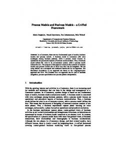
Figure 1 illustrates the subtraction factor ρ (γk , θk ) as a function of a posteriori SNR and relative angle θk . It can be concluded that ρ (γk , θk ) decreases monotonically as the a posteriori SNR increases. The

subtraction factor shows the asymptotic behavior: ρ (γk , θk ) ≈ − cos (θk ) γk ≫1 ρ (γk , θk ) = 1 − | cos (θk ) | − cos (θk ) γk =1

(13) (14)

In terms of the estimation rule implied by (7), for θk =π , which corresponds to the MSS solution [2], over-attenuation can be expected. Conversely, for θk =π/2, under-attenuation can be expected. Finally, for θk =0, (7) will tend to amplify noise components.

Motivated by the previous discussion, a subtraction factor, ρ˜ (γk ), is applied:

Rk = Ak + ρ˜k (γk ) Dk

(15)

where ρ˜k (γk ) is obtained by evaluating (10) at a certain relative angle. This yields modified definitions of a priori and a posteriori SNR: February 18, 2011

DRAFT

6

1

θ =π

k k

Subtraction Factor, ρ(γ ,θ )

k

θk=3π/4

0.5

θk=π/2

0

θk=π/4

−0.5

θk=0 −1 −40

Fig. 1.

−30

−20

−10

0

10

Instantaneous SNR, γk−1 (dB)

20

30

40

Subtraction Factors as a Function of γk and θk

ξ˜k = γ˜k =

σx2 (k) ρ˜2k (γk ) σn2 (k) ρ˜2k

(16)

Rk2 (γk ) σn2 (k)

Without prior knowledge of the relative phases of speech and noise components, ρ˜k offers the ability to tune the level of suppression applied during enhancement. Note that this term is similar to the concept of over-subtraction in [2] and [30]. In this study, a value of θk =7π/8 was empirically observed to provide promising results for estimating ρ˜k (γk ), when tested on the Noizeus database [28]. Note that in Sections III-V, STSA estimators are derived in terms of standard values of γk and ξk for the sake of consistency with existing solutions. However, a subtraction factor can be applied by using SNR values from (16).

B. Generalized Gamma Distributions Statistical modelling of spectral magnitudes has been widely studied for speech processing applications [5], [6], [10], [12].2 We utilize the generalized Gamma distribution during the derivation of optimal estimators, resulting in general solutions from which special cases can be obtained. In this way, we

2

Note that since this study deals with spectral magnitude estimation, only nonnegative distributions will be discussed. Thus,

unless otherwise explicitly noted, no reference to ”one-sided” will be made. February 18, 2011

DRAFT

7

1.5

(ζ=2,ν=1/2) (ζ=2,ν=1) (ζ=1,ν=1) (ζ=1,ν=2)

p(x)

1

0.5

0

0

1

0

1

2

3

4

2

3

4

p(x) (dB)

0

−50

−100

x

Fig. 2.

The Generalized Gamma Distribution for Various Shaping Parameter Pairs: For illustrative purposes, the variance was

normalized to unity.

increase the flexibility of the resulting estimators to varying signal types. The generalized Gamma distribution is given by:

p (x) =

( ) ζβ ν ζν−1 x exp −βxζ , Γ (ν)

(17)

for x ≥ 0; β, ν, ζ > 0, where Γ is the Gamma function. ν and ζ are referred to as shape parameters, and determine the overall shape of the distribution p (x), whereas β is referred to as the scale parameter, and is related to the noncentral second moment of the distribution. Specifically, the second moment of p (x) is given by [12]:   ] σ 2 = E x2 =  [

ν(ν+1) β2 , ν β , if ζ

if ζ = 1

(18)

=2

Figure 2 provides probability distribution functions (pdfs) of the GGD for various shaping parameter pairs. Specifically, the top panel shows p (x) in the linear scale, illustrating the effect of shaping parameters on GGDs. The bottom panel shows p (x) in the log scale, illustrating the relative prominence of distribution tails for each set of shaping parameters. Note that (17) is equivalent to that used in [12]. Further, it is similar to that used in [10], where scale parameters are defined differently. February 18, 2011

DRAFT

8

Studies in [10] and [9] provide empirical a priori distributions for speech and noise. Non-monotonic, unimodal distributions are shown for both speech and noise spectral amplitudes, similar to Erlang-2 and Rayleigh random variables. It should be noted, however, that empirical studies may often be greatly dependent on data, and may not convey true statistics. Therefore, we derive estimation solutions as functions of GGD shape parameters when mathematically possible. In this way, specific solutions can be obtained by substituting those shape parameters corresponding to expected speech and noise prior distributions. Alternatively prior distributions can be fitted according to ML or Kullback divergence criteria, as in [10]. In this study distinct distributions are used for noise and speech processes. Subscripts are utilized to denote shape parameters corresponding to noise (ζn , νn , βn ) or to speech (ζx , νx , βx ). Additionally, the proposed framework is robust to the use of channel-specific shape parameters. However, for the sake of simplicity, global parameters are utilized in this study. This paper presents a framework for determining optimal STSA estimators using the assumption of phase equivalence for speech and noise. Various combinations of GGD shape parameters for noise and speech processes lead to specific solutions. This study presents gain functions for those combinations which yield closed-form expressions. In the case of MMSE estimation, higher order shape parameters generally require numerical analysis since such expressions rely on integration. In the case of MAP estimation, certain combinations of lower order shape parameters result in a monotonic cost function for which a MAP solution does not exist. A summary of proposed estimators is provided in Table I.

III. ML E STIMATION In this section, we present ML short-time spectral estimators based on the aforementioned phase equivalence assumption. ML estimation offers an efficient framework for inferring unknown parameters when a priori distributions of the target signal are not known. From (7), it can be concluded that the conditional probability of observed spectral components, given underlying clean components, is simply dependent on noise statistics:

p (Rk |Ak ) = p (Dk = Rk − Ak ) =

(19)

( ) ζn βnνn (Rk − Ak )ζn νn −1 exp −βn (Rk − Ak )ζn Γ (νn )

ML estimation provides the estimate of Ak as: February 18, 2011

DRAFT

9

Aˆk = arg max F{p (Rk |Ak )}

(20)

Ak

where F{·} is monotonically increasing. Using F{·}=log (·) and (5) and (18), the ML solution is generalized as:

1 GM L (ξk , γk ) = 1− √ γk

( ζn

√

ζn νn − 1

)1/ζn

νn (νn + 2 − ζn )

,

(21)

for ζn ∈ {1, 2} Analysis of the second derivative of (19) reveals that for ζn νn < 1, the solution of (21) does not exist, since the distribution p (Rk |Ak ) is monotonic, and thus includes no maximum. For ζn =1 and νn =1, the GM L estimator reduces to unity.

It is interesting to note the similarity between the GM L estimator and magnitude spectral subtraction presented by Boll in [2]. Particularly, for large values of νn , which correspond to deterministic values of Ak without uncertainty, the proposed ML estimator approaches that given in [2].

GM L (ξk , γk )

√ ζn =2,νn →∞

=

γk − 1 √ γk

(22)

Figure 3 illustrates gain curves for the proposed ML STSA estimator for ζn =2, and for various values of the GGD shape parameter νn .

IV. MMSE E STIMATION In this section, we derive MMSE short-time spectral amplitude estimators assuming phase equivalence of speech and noise. In the general case, using (1), and assuming Ak and αk to be statistically independent, the MMSE estimate of Ak is determined as [6]:

Aˆk = E[Ak |Yk ] ∫ ∞ ∫ 2π Ak p (Yk |Ak , αk ) p (αk ) p (Ak ) ∂αk ∂Ak = 0∫ ∞ 0∫ 2π 0 0 p (Yk |Ak , αk ) p (αk ) p (Ak ) ∂αk ∂Ak

(23)

By assuming phase equivalence of speech and noise components, the distribution of αk and ψk are given by: February 18, 2011

DRAFT

10

0

−5

ν =3/2 Gain (dB)

n

ν =2 n

−10

ν =4 n

νn=∞

−15

−15

−10

−5

0

5

Instantaneous SNR, γk−1 (dB)

10

15

Fig. 3. Gain Curves for the GM L STSA Estimator, with ζn =2, and for Various Values of νn . Note that for νn =∞, the proposed M L estimator is equivalent to the magnitude spectral subtraction solution from [2].

p (αk ) = δ (αk − ηk )

(24)

p (ψk ) = δ (ψk − ηk )

(25)

where δ (·) represents the Kronecker delta function, and (23) simplifies to: ∫∞ Ak p (Rk |Ak ) p (Ak ) ∂Ak ˆ Ak = 0∫ ∞ 0 p (Rk |Ak ) p (Ak ) ∂Ak

(26)

Using (19), and the fact that Ak , Dk ∈ [0, Rk ], (23) reduces to: ∫ Rk Ak p (Dk = Rk − Ak ) p (Ak ) ∂Ak ˆ Ak = 0∫ Rk 0 p (Dk = Rk − Ak ) p (Ak ) ∂Ak

(27)

Assuming generalized Gamma distributions for speech and noise spectral magnitudes, the solution of (27) becomes: ( ) ζx νx ζx ζn νn −1 ζn A (R − A ) exp −β (R − A ) − β A ∂Ak n x k k k k k k 0 ( ) Aˆk = ∫ Rk ζx νx −1 (Rk − Ak )ζn νn −1 exp −βn (Rk − Ak )ζn − βx Aζkx ∂Ak 0 Ak ∫ Rk

(28)

(28) provides a general solution to MMSE spectral magnitude estimation assuming phase equivalence, and assuming priors from the generalized Gamma family. Particular solutions can be obtained by substituting specific statistical shape parameters corresponding to desired speech and noise distributions. February 18, 2011

DRAFT

11

Due to varying conclusions regarding the true statistical behavior of speech, we have avoided specifying models for speech and noise. Instead, (28) is provided as a function of GGD shape parameters. In the following subsections, we derive MMSE solutions for shape parameters which may be considered realistic for speech and noise.

A. Assuming Gaussian Noise Priors (ζn =2,νn =1/2) In this section, we derive the MMSE spectral magnitude estimator assuming Gaussian noise priors. Specifically, we present separate particular solutions assuming Gaussian and exponential speech priors, referred to as GGM M SE and GEM M SE , respectively. 1) Assuming Gaussian Speech Priors (ζx =2,νx =1/2): The GGMMSE solution, which utilizes Gaussian speech and noise priors, is derived from (28): ( ) 2 2 ∂A A exp −β (R − A ) − β A n x k k k k k 0 ( ) Aˆk = ∫ Rk 2 2 0 exp −βn (Rk − Ak ) − βx Ak ∂Ak ∫ Rk

(29)

Using (5) and (18), the integrals in (29) can be solved to reveal the GGMMSE gain function:

GGGM SE (ξk , γk ) =  ) ( ) ( √ γk γk ϕk exp − − exp − 2  2ϕk   ( 2ξk (1+ξk )) (√ ) ϕk − √  πγk  γk γk ϕk erf 2 2ξk (1+ξk ) + erf

(30)

where ϕk is the traditional Wiener filter (WF) [1]:

ϕk =

ξk . 1 + ξk

(31)

Additionally, erf (·) represents the Gauss error function: 2 erf (z) = √ π

∫

z

e−τ dτ. 2

(32)

0

It is interesting to note that for extreme values of the a posteriori SNR, the GGMMSE estimator approximates the Wiener filter: GGGM SE (ξk , γk ) February 18, 2011

|γ|≫1

≈ ϕk .

(33) DRAFT

12

More specifically, the GGMMSE gain function can be interpreted as the Wiener filter with an additive modification factor. To avoid a solution which includes irreducible functions, we approximate the Gauss error function by its truncated Taylor series expansion. The Taylor series expansion of the Gauss error function is given as [15]:

∞ 2 ∑ (−1)n z 2n+1 erf (z) = √ . n! (2n + 1) π

(34)

n=0

ˆ1 Using the 1st -order approximation, we derive the G GGM M SE solution:

ˆ 1GGM M SE (ξk , γk ) = G [ ( ( )) ( )] γk 1 + ξk2 1 γk (ξk − 1) ϕk 1 − exp − sinh γk 4ξk (1 + ξk ) 4ξk

(35)

The 1st -order approximation utilized in (35) can be expected to provide high accuracy for small values of γk , which correspond to acoustic conditions wherein the gain function is most important. ˆ1 Figure 4 illustrates gain curves for the G GGM M SE estimator, for various a priori SNRs. The Wiener ˆ1 filter is included for reference. As can be observed in Figure 4, the G GGM M SE converges to the Wiener

filter for large values of the a posteriori SNR. Additionally, for favorable acoustic conditions (eg. ξk =15 or ˆ1 5 dB), the G GGM M SE estimator provides increasing attenuation as the a posteriori SNR decreases, which

follows intuitively. For unfavorable conditions (eg. ξk =−5 or −15 dB), however, increased attenuation is applied for increasing a posteriori SNR. As discussed in [6], such behavior is the result of the estimator compromising between a priori information in the form of ξk , and new information introduced by γk . 2) Assuming Exponential Speech Priors (ζx = 1, νx = 1): Retaining the previous Gaussian model for the noise component and using (5) and (18), the GEMMSE solution can be adapted from (28) by assuming Exponential speech priors: ( ) 2 A exp −β (R − A ) − β A n x k k k k ∂Ak 0 ( ) Aˆk = ∫ Rk 2 0 exp −βn (Rk − Ak ) − βx Ak ∂Ak ∫ Rk

(36)

The GEMMSE gain function can be derived from (36) as: February 18, 2011

DRAFT

13

0

ξk=15 dB ξk=5 dB

Gain (dB)

−5

ξ =−5 dB

−10

k

ξk=−15 dB

−15

−20

Fig. 4.

−15

−10

−5

0

5

instantaneous SNR, γk−1 (dB)

10

15

20

ˆ 1GGM M SE STSA estimator (solid line) for various values of ξk : The Wiener filter [1] (dotted Gain curves for the G

line) is included for comparison.

√

2 GGEM M SE (ξk , γk ) = 1 − ξk γk ( ) ( ) √  γk √ 1 1 √2γk exp − − exp − − + ξk 2 ξk 2  ξ ( ) (√ )k  − γk πγk erf √1 + erf − √1 ξk

2

(37)

ξk

As in the previous section, the GEMMSE includes irreducible Gauss error functions, which can be expressed as Taylor series expansions [15]. Following the steps from the previous section, the GEMMSE solution can be approximated as:

ˆ 1GEM M SE (ξk , γk ) = 1 − √ 1 G 2 ξk γk [ ( ) ( )] √ √ γk γk γk 1 1 γk − exp − − + sinh − γk ξk 4 2ξk 4 2ξk

(38)

Figure 5 illustrates gain curves for the GEM M SE 1 estimator for various values of ξk . It is interesting to note the dissimilarities in behavior between the GEM M SE 1 and GGM M SE 1 solutions. The increased attenuation applied by the former is due to the narrow peak of the exponential distribution, which shifts spectral estimates downward. February 18, 2011

DRAFT

14

0

ξk=15 dB ξk=5 dB

Gain (dB)

−5

ξk=−5 dB −10

ξk=−15 dB

−15

−20

Fig. 5.

−15

−10

−5

0

5

Instantaneous SNR, γk−1 (dB)

10

15

20

ˆ 1GEM M SE STSA estimator for various values of ξk Gain curves for the G

B. Assuming Exponential Noise Priors (ζn = 1, νn = 1) In this section, we derive a general MMSE solution assuming exponential noise spectral magnitude priors, with speech prior distributions constrained by ζx =1, but given as a function of νx ∈ N1 , where N1 is the set of natural numbers. Note that for ζx =2, the MMSE estimator is irreducible, and numerical approximation must be used to obtain a solution. For ζx =1, (28) can be simplified as:

∫ Rk νx A exp (− (βx − βn ) Ak ) ∂Ak ˆ Ak = ∫ R0k ν k−1 x exp (− (βx − βn ) Ak ) ∂Ak 0 Ak

(39)

The following identity, which is proven in Appendix II, is helpful in deriving the current spectral estimator:

∫ 0

z

τ m exp (cτ ) dτ =  [  exp(cz) ∑m (−1)h h=0 c



z m+1 ,

(40) m! z m−h (m−h)! ch

]

, for c ̸= 0

for c = 0

Using (5), (18), (39), and (40), the MMSE STSA estimator for exponential noise priors can be expressed as: February 18, 2011

DRAFT

15

ξ =15 dB k

−5

ξ =5 dB

Gain (dB)

k

ξ =−5 dB k

−10

ξk=−15 dB

−15

−20

Fig. 6.

−15

−10

−5

0

5

Instantaneous SNR, γk−1 (dB)

10

15

20

(ν )

x Gain Curves for the GEM M SE STSA Estimator for νx =1 (solid line) and νx =2 (dotted line)

(ν )

x GEM M SE (ξk , γk ) = )  [ ] ∑ x ( x! (−1)νx νx !+exp(µk ) νh=0 (−1)h (ν ν−h)! µνkx −h  1 x  ( ) ,  ∑ x −1 x −1)!  (−1)h (ν(ν−h−1)! µkνx −h−1  µk (−1)νx −1 (νx −1)!+exp(µk ) νh=0 x

    

(41)

for c ̸= 0 νx νx +1

for c = 0

where: √ µk =

2γk ξk

( √

√ ξk −

νx (νx − 1) 2

) .

(42)

Note that the gain function in (41) is expressed as a function of νx , which allows flexibility in modelling the speech component. We present an example EMMSE solution for νx =1, which corresponds to an exponential speech prior:

(νx =1) GEM M SE

1 = µk

(

−1 + exp (µk ) (−1 + µk ) 1 + exp (µk )

) ,

(43)

(ν )

x Figure 6 provides gain curves for the GEM M SE estimator, for νx ={1, 2}. As can be observed, with

increasing νx , the estimator generally provides decreased attenuation. This is due to the corresponding a priori speech distribution shifting its mode outward, thereby increasing the expected value of Ak . February 18, 2011

DRAFT

16

V. MAP E STIMATION Maximum a posteriori estimation offers mathematically efficient solutions to problems which may not be feasible via other means. In this section, we present a group of MAP spectral amplitude estimators assuming phase equivalence of speech and noise. We explore Gaussian and Rayleigh noise priors. As with MMSE estimation, higher order shape parameters offer valid solutions; however, higher order GGDs typically result in solutions which can not be expressed in closed form. MAP estimation determines the solution Aˆk which maximizes the expression p (Rk |Ak ) p (Ak ), or some monotonic function thereof, given the observation Rk :

Aˆk = arg max F{p (Rk |Ak ) p (Ak )}, Ak

(44)

= arg max F{p (Dk = Rk − Ak ) p (Ak )}, Ak

where F is monotonic. We utilize the logarithmic function during MAP estimation:

Aˆk = Ak such that

∂ C (Ak ) = 0, ∂Ak

(45)

where C (Ak ) = log (p (Rk |Ak ) p (Ak )) Assuming generalized Gamma priors for speech and noise components and using (17) and (19), the equality

∂ ∂Ak C

(Ak )=0 is expressed as:

ζx νx − 1 ζn νn − 1 − − βx ζx Aζkx −1 Ak Rk − A k

(46)

+ βn ζn (Rk − Ak )ζn −1 = 0

Analyzing the 2nd derivative of C (Ak ) with respect to Ak leads to:

∂2 ζx νx − 1 ζn νn − 1 C (Ak ) = − − ∂A2k A2k (Rk − Ak )2

(47)

− βx ζx (ζx − 1) Aζkx −2 − βn ζn (ζn − 1) (Rk − Ak )ζn −2

(47) shows that

∂2 ∂A2k C

(Ak ) will be guaranteed to be negative, and the solution from (46) valid, if each

of the following inequalities holds: February 18, 2011

DRAFT

17

(i) ζx ≥ 1

(48)

(ii) ζn ≥ 1 (iii) ζx νx ≥ 1 (iv) ζn νn ≥ 1

(47) can assume negative values even if certain constraints in (48) are not met; however, these inequalities offer a simple check which encompasses the majority of valid speech and noise GGD shape parameters.

A. Assuming Gaussian Noise Priors (ζn =2,νn =1/2) In this section, we present a family of MAP spectral magnitude estimators assuming Gaussian noise prior distributions. We derive separate general solutions for speech distributions constrained by (ζx =2, νx ∈ R) and (ζx =1, νx ∈ R). The G2M AP estimator is derived from the assumption of Gaussian noise and speech distributions constrained by (ζx =2, νx ∈ R). In this case, applying (5) and (18) to (46) leads to:

A2k −

ξk ξk (2νx − 1) 2 Rk A k − R =0 2νx + ξk γk (2νx + ξk ) k

(49)

Applying the quadratic equation, and choosing the nonnegative root, yields:

(ν )

x GG2M AP (ξk , γk )

ξk + =

√

(50) ξk2 + 4 (ξk /γk ) (2νx − 1) (2νx + ξk ) 2 (2νx + ξk )

(ν )

x It is interesting to note that the GG2M AP estimator of (50) shows striking similarity to the MAP STSA

estimator proposed by Wolfe and Godsil in [8]. Furthermore, the case of νx =1/2 leads to the Wiener filter

(ν =1/2)

x GG2M AP (ξk , γk ) = ϕk

(51)

(ν )

x Figure 7 illustrates gain curves for the GG2M AP STSA estimator for νx =1 (solid line), νx =2 (dashed

line), and νx =3 (dotted line). February 18, 2011

DRAFT

18

5 ξ =15 dB k

0

Gain (dB)

−5

ξk=5 dB

ξk=−5 dB

−10

ξk=−15 dB

−15

−20 −20

Fig. 7.

−15

−10

−5 0 5 instantaneous SNR, γk−1 (dB)

10

15

20

(ν )

x Gain curves for the GG2M AP STSA estimator for νx =1 (solid line), νx =1 (dashed line), and νx =3 (dotted line)

The steps involved in deriving MAP spectral estimators, which were previously followed to obtain the G2M AP solution, are summarized below:

1) Choose GGD size parameters corresponding to desired speech and noise prior distributions, and check for validity (48). 2) Substitute GGD size parameters into the general solution for MAP estimation (46). 3) Solve (46) for Aˆk . Note that in certain cases, such as when

∂ ∂Ak C

(Ak ) is linear or quadratic, this

can be done in closed form. Other cases may rely on numerical approximations. 4) If multiple roots are obtained for Aˆk choose the root which falls within the desired range [0, ∞). 5) Substitute the definitions of the a priori and a posteriori SNRs (Sec. II) into Aˆk . Following the previously outlined steps, the G1M AP solution is derived from the assumption of (ζx = 1, νx ∈ R):

(ν )

x GG1M AP (ξk , γk ) =

v( )2 u √ √ νx (νx + 1) u νx (νx + 1) 1 1 (νx − 1) t √ √ + − − + 2 2 γk 2 γk ξk 2 γk ξk

(52)

(ν )

x Figure 8 illustrates gain curves for the GG1M AP STSA estimator for νx =1.5 (solid line), νx =2.0 (dashed

line), and νx =2.5 (dotted line). February 18, 2011

DRAFT

19

5

ξk=15 dB

0

Gain (dB)

−5

ξk=5 dB −10

ξk=−5 dB

−15

−20

ξk=−15 dB −25 −20

Fig. 8.

−15

−10

−5

0

5

instantaneous SNR, γk−1 (dB)

10

15

20

(ν )

x Gain curves for the GG1M AP STSA estimator for νx =1.5 (solid line), νx =2.0 (dashed line), and νx =2.5 (dotted line)

B. Assuming Rayleigh Noise Priors (ζn = 2, νn = 1) In this section, we present a family of MAP spectral magnitude estimators assuming Rayleigh noise prior distributions. (46) now reduces to: (ζx νx − 1) − βx ζx Aζkx −

Ak + 2βn Ak (Rk − Ak ) = 0. Rk − Ak

(53)

It can be observed that the expression in (53) is a (ζx + 1)th -order polynomial. However, if the speech distribution shape parameters are constrained such that ζx νx = 1, the expression can be reduced to a ζxth -order polynomial, and its roots can be obtained more efficiently. If Gaussian speech prior distributions

are assumed, the RGM AP solution can be derived according to the steps outlined in Section V-A:

GRGM AP

( ) 1 4ξk + 1 (ξk , γk ) = 2 2ξk + 1 √( ) ( ) 4ξk + 1 2 4ξk 2γk − 1 1 + − 2 2ξk + 1 γk 2ξk + 1

(54)

Instead if exponential speech priors are assumed, the REM AP estimator is derived as:

1 GREM AP (ξk , γk ) = 1 − √ 2 2ξk γk √( ) )2 ( 1 1 1 + −1 1− √ + + √ 2γk 2 2ξk γk 2ξk γk February 18, 2011

(55)

DRAFT

20

0

Gain (dB)

−5

ξk=15 dB ξk=−5 dB

−10

ξk=−15 dB −15

ξk=5 dB

−20

−25 −20

Fig. 9.

−15

−10

−5

0

5

Instantaneous SNR, γk−1 (dB)

10

15

20

15

20

Gain curves for the GRGM AP STSA estimator for various values of ξk

0

−5

Gain (dB)

ξk=15 dB −10

ξ =5 dB k

−15

ξ =−5 dB k

ξk=−15 dB

−20

−25 −20

Fig. 10.

−15

−10

−5

0

5

Instantaneous SNR, γk−1 (dB)

10

Gain curves for the GREM AP STSA estimator for various values of ξk

(ν )

x It is interesting to note the similarity between the proposed GG1M AP and GREM AP (ξk , γk ) solutions,

and the joint-MAP (JMAP) STSA estimator proposed by Lotter and Vary in [10]. Figures 9 and 10 illustrate gains curves for the GRGM AP and GREM AP estimators, respectively. Table I provides a summary of the generalized STSA estimators derived in Sections III, IV, and V. VI. E XPERIMENTAL R ESULTS In order to assess the success of the proposed spectral estimators, they are tested on the Noizeus database [28]. The Noizeus database is comprised of phonetically balanced utterances, and includes 8 types of non-stationary additive noise. Proposed STSA estimators were embedded into code from [32], February 18, 2011

DRAFT

21

TABLE I S PECTRAL M AGNITUDE E STIMATORS D ERIVED IN S ECTIONS III, IV, AND V: PARTICULAR SOLUTIONS ARE OBTAINED BY SUBSTITUTING INTO GENERAL SOLUTIONS THOSE STATISTICAL PARAMETERS CORRESPONDING TO DESIRED NOISE AND SPEECH PRIORS .

N OTE THAT ζn AND νn REFER TO GGD SHAPE PARAMETERS CORRESPONDING TO THE NOISE PROCESS ,

AND ζx AND νx REFER TO

GGD SHAPE PARAMETERS CORRESPONDING TO THE SPEECH PROCESS .

Criterion

(ζn , νn )

(ζx , νx )

Name

ML

(ζn ∈ {1, 2}, νn ≥ 1/ζn )

-

GM L

(2, 1/2)

ˆ 1GGM M SE G

(1, 1)

ˆ 1GEM M SE G

(2, 1/2)

(ν )

MMSE (1, 1)

(2, 1/2) MAP

(2, 1)

(1, νx ∈ N1 )

x GEM M SE

(ν )

(2, νx ∈ R)

x GG2M AP

(1, νx ∈ R)

x GG1M AP

(2, 1/2)

GRGM AP

(1, 1)

GREM AP

(ν )

G (ξk , γk )

)1/ζn √ ζn νn −1 [ ( ζn νn (ν2n +2−ζ ) n) ( )] γ 1+ξ ( ) k γk (ξk −1) k 1 ϕk 1 − γk exp − 4ξk (1+ξk ) sinh 4ξk [ ( ) ( )] √ √ γ γk γ 1 − √1 − γ1k exp − ξ1k − 4k + 2ξkk sinh γ4k − 2ξ k 2 ξk γ k ) ( ) ∑ νx ( νx −k νx ! νx k (

1−

1 µk

(−1)

1 √ γk

νx !+exp(µk )

(−1)νx −1 (νx −1)!+exp(µk )

(−1) (ν −k)! µk k=0 x ) ∑νx −1 ( (νx −1)! ν −k−1 µkx (−1)k (ν −k−1)! k=0

( ) √ x √ √ νx (νx −1) k where µk = 2γ ξ − k ξk 2 ( ) √ 1 ξk + ξk2 + 4 (ξk /γk ) (2νx − 1) (2νx + ξk ) 2(2νk +ξk ) √( )2 √ √ νx (νx +1) νx (νx +1) 1 1 √ √ − + − + (νxγ−1) 2 2 k 2 γk ξk 2 γ k ξk √( ( ) ) ( ) 1 2

1− √1 2

2

4ξk +1 k + 21 − 4ξ 2ξk +1 γk √( )2 ( + 1− √1 + √

4ξk +1 2ξk +1

2ξk γk

2

2ξk γk

2γk −1 2ξk +1

1 2ξk γk

which applies a gain floor of −18 dB and performs improved minima controlled recursive averaging (IMCRA) noise estimation [33]. The enhancement system applies 20 ms analysis windows with 15 ms overlap. A fast Fourier transform (FFT) of length 256 is used during spectral decomposition. Results were averaged across 30 utterances, and 8 noise types. In order to analyze the effect of enhancement on speech and noise components separately, we use SSNR-related metrics defined in [10]. Specifically, along with the overall SSNR measure, we consider separately the SSNR of active speech frames (SSNRX ) and inactive speech frames (SSNRN ). For an enhanced speech signal x ˆ (n) and clean reference signal x (n), the global SSNR is defined as: February 18, 2011

DRAFT

+

1 2γk

) −1

22

SSN R = [ ( )] ∑Nw 2 Nf 1 ∑ i=1 x (i + kNh ) 10 log10 ∑Nw Nf ˆ (i + kNh ))2 i=1 (x (i + kNh ) − x

(56)

k=1

where Nw is the length of the analysis window, Nh is the shift in samples for each successive window, and Nf is the number of frames analyzed. The SSNRX is determined similarly to (56), although only computed for speech frames wherein the clean signal energy is ≥ −30 dB [10]. Conversely, the SSNRN is computed only for frames exhibiting energy < −30 dB. Table II provides quantitative results for a subset of the proposed STSA estimators, when applied to the Noizeus database [28]. The subset of proposed estimators was chosen to represent a diverse group. Note that most often the proposed MMSE- and MAP-based estimators outperform the ML-based estimator. However, for estimation of general signals, the ML solution is applicable when a priori statistics of the signal of interest are unknown. ∆, ∆X , ∆N refer to improvements in SSNR, SSNRX , SSNRN , respectively, relative to the unprocessed signal. Bold entries denote the best score for each metric at each noise condition. Results in Table II were obtained with a subtraction factor ρk (γk , θk ) evaluated at θk =7π/8, as discussed in (15) and (16).

Table II shows the proposed STSA estimators to generally provide improved overall signal quality (SSN R) and noise suppression (SSN RN ), relative to the LMMSE solution from [7], the MAP solution from [8], and the JMAP solution from [10]. The proposed methods provide generally improved active speech quality (SSN RX ) relative to [7]. The GGM M SE 1 estimator, which provides the best scores, outperforms that from [7] by approximately 1-2.5 dB in terms of SSN R across noise levels, and by approximately 5-6.5 dB in terms of SSN RN . It should be noted that for some noise levels, the solutions from [8] and [10] lead to slightly better SSN RX scores, relative to the proposed estimators. In these cases, the proposed solutions may be attenuating speech components while attempting to suppress noise components. In the proposed approach, the subtraction factor ρ˜k can be tuned to control the tradeoff between noise suppression and speech distortion. STSA estimators are also evaluated using a discretized version of the COSH distance from [34]: Nch 1 ∑ dCOSH (x (n) , x ˜ (n)) = 2Nch k=1

(

Ak Aˆk −2 + Ak Aˆk

) (57)

where Nch is the number of channels used during spectral analysis. Table III provides COSH measures for a subset of the proposed STSA estimators, when applied to the Noizeus database [28]. Bold entries February 18, 2011

DRAFT

23

TABLE II S EGMENTAL SNR S CORES FOR S ELECTED STSA E STIMATORS : ∆, ∆X , ∆N REFER TO IMPROVEMENTS IN SSNR, SSNRX , SSNRN , RESPECTIVELY, RELATIVE TO THE UNPROCESSED SIGNAL . R ESULTS WERE OBTAINED ON THE N OIZEUS DATABASE

[28]. T HE SUBSET OF ESTIMATORS INCLUDED WERE SELECTED FROM THE PROPOSED FRAMEWORK TO

REPRESENT A DIVERSE MIX .

B OLD ENTRIES DENOTE THE BEST SCORE FOR EACH METRIC AT EACH NOISE CONDITION .

Input SNR 15 dB

10 dB

5 dB

0 dB

Estimator

(ζn , νn )

(ζx , νx )

∆

∆X

∆N

∆

∆X

∆N

∆

∆X

∆N

∆

∆X

∆N

LM M SE [7]

−

−

4.8

2.5

10.6

5.6

3.4

10.8

6.5

4.5

11.1

7.3

5.7

11.0

M AP [8]

−

−

4.8

2.5

10.6

5.6

4.5

10.8

6.5

5.0

11.1

7.3

6.4

11.0

JM AP [10] ˆ 1GGM M SE G

−

−

4.9

2.5

10.8

5.7

4.6

11.1

6.5

5.0

11.3

7.3

6.4

11.3

(2, 1/2)

(2, 1/2)

5.2

1.8

13.7

6.3

3.0

14.4

7.4

4.4

15.0

8.6

6.0

15.0

(νx =1) GEM M SE (νx =1/2) GG2M AP

(1, 1)

(1, 1)

4.7

2.5

10.0

5.4

3.4

10.1

6.2

4.4

10.2

6.9

5.5

10.1

(2, 1/2)

(2, 1/2)

5.2

2.5

11.9

6.1

3.5

12.3

7.0

4.7

12.6

7.9

5.9

12.6

GRGM AP

(2, 1)

(2, 1/2)

5.1

2.5

11.6

5.9

3.5

11.8

6.8

4.7

12.1

7.7

5.8

12.0

GREM AP

(2, 1)

(1, 1)

4.9

2.5

10.7

5.6

3.4

10.9

6.4

4.5

11.0

7.2

5.6

10.9

denote the best score for each metric at each noise condition. It can be observed that several of the proposed estimators provide lower distortion measures than the previously mentioned baseline solutions, ˆ1 across all noise levels. Furthermore, the best results are achieved by the G GGM M SE estimator.

Informal listening tests show the proposed estimators included in Table II to provide a noticeable improvement in noise suppression, across noise types and levels, relative to the solutions from [7], [8], and [10]. Speech enhancement at low noise levels (5 dB and 0 dB), did result in some apparent musical noise, especially for highly non-stationary, speech-shaped noise types, such as babble and restaurant. However, this musical noise was generally not more noticeable than that produced by the baseline methods. VII. S UMMARY AND D ISCUSSION In this paper, we present a stochastic framework for designing optimal spectral magnitude estimators for speech enhancement assuming equivalent phase of speech and noise components. By assuming phase equivalence, we effectively project the optimal spectral amplitude estimation problem onto a 1dimensional subspace of the complex plane, thus simplifying the problem formulation. We derive separate families of novel estimators assuming generalized gamma distributions (GGDs) for both speech and noise February 18, 2011

DRAFT

24

TABLE III COSH D ISTORTION M EASURES [34] FOR THE STSA E STIMATORS I NCLUDED IN TABLE II. R ESULTS WERE OBTAINED ON THE

N OIZEUS DATABASE [28]. B OLD ENTRIES DENOTE THE BEST SCORE FOR EACH METRIC AT EACH NOISE CONDITION .

Input SNR (dB) Estimator

(ζn , νn )

(ζx , νx )

15

10

5

0

LM M SE [7]

−

−

1.43

2.65

4.55

8.13

M AP [8]

−

−

1.45

2.78

4.55

8.10

JM AP [10] ˆ 1GGM M SE G

−

−

1.44

2.61

4.46

7.93

(2, 1/2)

(2, 1/2)

1.33

2.07

3.26

5.48

(νx =1) GEM M SE (νx =1/2) GG2M AP

(1, 1)

(1, 1)

1.47

2.74

4.81

8.63

(2, 1/2)

(2, 1/2)

1.39

2.37

3.97

6.93

GRGM AP

(2, 1)

(2, 1/2)

1.39

2.41

4.10

7.23

GREM AP

(2, 1)

(1, 1)

1.45

2.58

4.48

7.95

spectral magnitudes, according to the ML, MMSE, or MAP criterion. Solutions are provided in general form, so that estimators can be obtained by substituting statistical shape parameters corresponding to desired speech and noise priors. Table I provides an overview of the novel estimators derived in this paper. It is interesting to note the similarity between certain proposed estimators, and traditional solutions such as MSS [2], the Wiener filter [1], and MAP estimators presented in [8] and [10]. Quantitative analysis of the proposed estimators generally shows improvement in terms of segmental SSNR and COSH distance, when applied to the Noizeus database [28]. Informal listening tests showed proposed estimators to provide apparent improvement in noise suppression, relative to [7]. Though some musical artifacts were present at low SNRs, it was generally less noticeable than for [7]. Additionally, the subtraction factor was applied to decrease the over-attenuation common with spectral subtraction-based methods, improving both quantitative and perceptual results. Traditionally, Gaussian pdfs were used to model real and imaginary components of speech and noise DFT coefficients. This corresponds to Rayleigh-distributed spectral magnitudes. More recent work has suggested super-Gaussian pdfs for spectral magnitudes. In our paper, the best results are obtained for the one-sided Gaussian distribution for spectral magnitudes of speech and noise. This case can in many respects be considered to lie between the two previously mentioned cases. February 18, 2011

DRAFT

25

The flexibility of the proposed framework makes it applicable to estimating arbitrary signals corrupted by additive noise. Given the expected shape parameters of the target and noise STSA distributions, an optimal spectral magnitude estimator can be derived. Possible extensions of the presented work include enhancement of general audio signals, such as music enhancement [8],[25], and image denoising [26],[27]. A PPENDIX I D ERIVATION OF (10) Using a geometric approach to spectral subtraction, and applying the law of cosines leads to:

Rk2 = A2k + Dk2 − 2Ak Dk cos θk

(58)

Solving for Ak using the quadratic equation results in: √ Ak = Dk cos θk +

D2 cos2 θk − Dk2 + Rk2

(59)

Grouping terms in (59) to match those in (8), with γk =Rk2 /Dk2 yields: ( Ak = Rk −

√

γk −

√

) γk − sin θk − cos θk Dk 2

(60)

A PPENDIX II D ERIVATION OF THE I DENTITY IN (40) Define the integral Im as: ∫

z

Im =

xm exp (cx) dx.

(61)

z m+1

(62)

0

For c=0, the integral can be easily solved as: Im

c=0

=

For c ̸= 0, the integral can be expressed recursively as: Im

  c̸=0

=



m 1 m c z exp (cz) − c Im−1 , 1 c (exp (cz) − 1) , for m

for m > 0

.

(63)

=0

Using (63), Im can be grouped concisely into a summation: February 18, 2011

DRAFT

26

  Im =



exp(cz) c z m+1 ,

∑m [ h=0

(−1)h

m! z m−h (m−h)! ch

]

, for c ̸= 0

(64)

for c = 0 R EFERENCES

[1] N. Wiener, Extrapolation, Interpolation, and Smoothing of Stationary Time Series, Wiley, 1949. [2] S. F. Boll, Suppression of Acoustic Noise in Speech Using Spectral Subtraction, IEEE Trans, on Acoustics, Speech, and Signal Processing, Vol. 27, pp. 113-120, 1979. [3] M. Berouti, R. Schwartz, and J. Makhoul, Enhancement of speech corrupted by acoustic noise, ICASSP, pp. 208-211, 1979. [4] Y. Lu, and P. Loizou, A geometric approach to spectral subtraction, Speech Communication, Vol. 50, pp. 453-466, 2008. [5] R. J. McAulay and M. L. Malpass, Speech Enhancement Using a Soft-Decision Noise Suppression Filter, IEEE Trans. on Acoustics, Speech, and Signal Processing, Vol. 28, No.2, pp. 137-145, 1980. [6] Y. Ephraim and D. Malah, Speech Enhancement Using a Minimum Mean-Square Error Short-Time Spectral Amplitude Estimator, IEEE Trans. on Acoustics Speech, and Signal Processing, Vol. 32, No. 6, pp. 1109-1121, 1984. [7] Y. Ephraim and D. Malah, Speech Enhancement Using a Minimum Mean-Square Error Log-Spectral Amplitude Estimator, IEEE Trans. on Acoustics, Speech, and Signal Processing, Vol. 33, No. 2, pp. 443445, 1985. [8] P. J. Wolfe and S. J. Godsil, Efficient Alternatives to the Ephraim and Malah Suppression Rule for Audio Signal Enhancement, EURASIP J. Appl. Signal Processing, No. 10, pp. 1043-1051, 2003. [9] R. Martin, Speech Enhancement Based on Minimum Mean-Square Error Estimation and Supergaussian Priors, IEEE Trans. on Speech and Audio Processing, Vol. 13, No. 5, pp. 845-856, 2005. [10] T. Lotter and P. Vary, Speech Enhancement by MAP Spectral Amplitude Estimation Using a Super-Gaussian Speech Model, EURASIP Journal on Applied Signal Processing, Vol. 7, pp. 1110-1126, 2005. [11] I. Cohen, Speech Enhancement Using Super-Gaussian Speech Models and Noncausal a Priori SNR Estimation, Speech Communication, Vol. 47, pp. 336-350, 2005. [12] J. S. Erkelens, R. C. Hendriks, R. Heusdens, and J. Jensen, Minimum Mean-Square Error Estimation of Discrete Fourier Coefficients with Generalized Gamma Priors, IEEE Trans. Audio, Speech, and Language Processing, Vol. 15, No. 6, pp. 1741-1752, 2007. [13] T. H. Dat, K. Takeda, and F. Itakura, Generalized Gamma Modelling of Speech and its Online Estimation for Speech Enhancement, ICASSP, Vol. IV, pp. 181-184, 2005. [14] B. Chen and P. C. Loizou, A Laplacian-based MMSE Estimator for Speech Enhancement, Speech Communication, Vol. 49, pp. 134-143, 2007. [15] M. Abromowitz and I. A. Stegun, Handbook of Mathematical Functions, Dover, 1972. [16] E. D. Solomenstev, Cauchy Inequality, in Encyclopedia of Mathematics, Kluwer Academic Publishing, 2001. [17] P. Vary, Noise Suppression by Spectral Magnitude Estimation- Mechanism and Theoretical Limits, Signal Processing, Vol. 8, pp. 387-400, 1985. [18] D. L. Wang and J. S. Lim, The Unimportance of Phase in Speech Enhancement, IEEE Trans. Acoustics, Speech, and Signal Processing, Vol. 30, No. 4, pp. 679-681, 1982. [19] ITU-T Rec P.862 Perceptual evaluation of speech quality (PESQ), and objective method for end-to-end speech quality assessment of narrowband telephone networks and speech codecs. February 18, 2011

DRAFT

27

[20] H.-G. Hirsch and D. Pearce, The AURORA Experimental Framework For The Performance Evaluation of Speech Recognition Systems Under Noisy Conditions, ASR2000 - Automatic Speech Recognition: Challenges for the new Millenium, 2000. [21] L. Rabiner and B. H. Juang, Fundamentals of Speech Recognition, Prentice Hall, 1993. [22] D. Pearce, Enabling New Speech Driven Services For Mobile Devices: An Overview of the ETSI Standards Activities for Distributed Speech Recognition Front-Ends, AVIOS 2000: Speech Appl. Conf., Vol. 5, May 2000. [23] D. Middleton and R. Esposito, Simultaneous optimum detection and estimation of signals in noise, IEEE Trans. on Information Theory, vol. 14, pp. 434-444, 1968. [24] J. Sohn, N. S. Kim, and W. Sung, A Statistical Model-Based Voice Activity Detection, IEEE Signal Processing Letters, Vol. 6, No. 1, pp. 1-3, 1999. [25] S.-H. Oh, W.-J. Yoan, Y.-H. Cho, and K.-S. Park, A New Spectral Enhancement Algorithm in MP3 Audio, ICCE, pp. 285-286, 2006. [26] A. K. Jain, Fundamentals of Digital Image Processing, Prentice Hall, 1989. [27] R. Okten, L. Yaroslavsky, K. Egiazarian, and J. Astola, Transform Domain Approaches for Image Denoising, Journal of Electronic Imaging, 11(2), pp. 149-156, 2002. [28] Y. Hu and P. Loizou, Subjective evaluation and comparison of speech enhancement algorithms, Speech Communication, vol. 49, pp. 588-601, 2007. [29] S. Kamath and P. Loizou, A multi-band spectral subtraction method for enhancing speech corrupted by colored noise, ICASSP, 2002. [30] P. Lockwood, J. Boudy, and M. Blanchet, Non-linear spectral subtraction (NSS) and Hidden Markov Models for robust speech recognition in car environments, ICASSP, vol. I, pp. 265-268, 1992. [31] I. S. Gradshteyn and I. M. Ryzhik, Table of Integrals, Series and Products, Academic Press, 2000. [32] http://webee.technion.ac.il/Sites/People/IsraelCohen/ [33] I. Cohen,Optimal speech enhancement under signal presence uncertainty usinglog-spectral amplitude estimator, IEEE Signal Processing Letters, Vol. 9, Issue 4, pp. 113-116, 2002. [34] A. H. Gray and J. D. Markel, Distance Measures for Speech Processing, IEEE Trans. on Acoustics, Speech, and Signal Processing, Vol. 24, No. 5, pp. 380-391, 1976.

February 18, 2011

DRAFT