A Unified Framework for Line Extraction in Dioptric and Catadioptric Cameras J. Bermudez-Cameo, G. Lopez-Nicolas and J.J. Guerrero Instituto de Investigaci´ on en Ingenier´ıa de Arag´ on Universidad de Zaragoza, Spain Email:
[email protected],
[email protected],
[email protected]
Abstract. Many of the omnidirectional visual systems have revolution symmetry and, consequently, they can be described by the radially symmetric distortion model. Following this projection model, straight lines are projected on curves called line-images. In this paper we present a novel unified framework to deal with these line-images directly on the image which is valid for any central system. In order to validate this framework we have developed a method to extract line-images with a 2-points RANSAC, which makes use of the camera calibration. The proposed method also gives the adjacent regions of line-images which can be used for matching purposes. The line-images extractor has been implemented and tested with simulated and real images.
1
Introduction
Line-images have been extensively used in computer vision. When a projection system is central, the 3D line and the view-point (optical center) lies on the same plane Π and the projection is described by a vector normal n to this plane Π. In general, any point X contained in plane Π is projected on the line-image and satisfies a nice constraint like nT X = 0. In perspective cameras this constraint is transformed to the image plane resulting a 2D line. When the projection system is not perspective the relationship is not linear and the projected line-image is a curve. Many approaches, e.g [1, 2], solve the constraint for collinear points in the unitary sphere. The intersection of the plane Π with the unitary sphere is a great circle which is related with the image using the projection model. Instead of working on the sphere the problem can be tackled directly on the image. This approach has been extensively used in catadioptric images. The catadioptric line projection is modelled by the proposal of Geyer et al. [3]. In this particular case line-images are conics [4, 5]. For the case of fisheyes, line-images have not been extensively used. Most of conventional and non-conventional cameras have revolution symmetry. Even when this constraint is not perfectly satisfied differences with the model can be encapsulated in an additional linear transformation. Main advantage of radially symmetric distortion is that can be used to model many different devices including perspective cameras, fisheyes and catadioptric systems.
2
J. Bermudez-Cameo, G. Lopez-Nicolas and J.J. Guerrero
X
Z
xˆ
hyper
xˆ x π
radial
xˆ
pers
ϕ
ϕ
φ
x X
O
sphere
1
Y
ϕ
ξ
Fig. 1. Catadioptric sphere camera model: The 3D point X is projected onto the sphere. Then this point is backprojected to a normalized plane through a virtual optic center located a distance ξ from the effective viewpoint. This point x ¯ is transformed to the image plane using the collineation Hc . Fisheye camera models: The radius of the point on the image is distorted by a function rˆ = h (ϕ).
As the line projection on the raw image is defined by more than two points it contains information about the calibration and distortion model and can be used to correct the image distortion [6–8]. These works are not about the line-image as geometric form, however the line-image is implicitly contained in them. In spite of not being expressed explicitly, the workspace used in Tardif et al. [9] is very related with the space in which a line-image is represented in our proposal. Once the line-projection model is performed one direct application is lineimage extraction. When the direct line projection model is known a Hough transform approach could be used for line-detection. This is the approach used for line-extraction with catadioptric systems in [10–12]. In [2] a scheme of split and merge is proposed to extract line-images in catadioptric systems. This approach use the inverse point projection model to back-project the points to the unitary sphere where the robust fitting is done. In [13, 14] a line-extraction method for hypercatadioptric systems solving the equation of the conic on the normalizedplane is proposed. In this paper, we present a framework for line-image extraction in central systems following radially symmetric distortion models. This unified framework is a generalisation of the method presented by Bermudez-Cameo et al. in [13]. This generalisation expands the results obtained for hypercatadioptric systems to other catadioptric systems and dioptric systems with revolution symmetry. Explicit analytic expressions have been obtained for paracatadioptric, equiangular-
A Unified Framework for Line Extraction ...
3
fisheye, stereographic-fisheye and orthogonal-fisheye models. We show an expression for the homogeneous line-image equation which is coherent with radially symmetric distortion models. The image-space in which the line-image is represented is similar to the space used in [9] for self-calibration. Main difference with this work is that we focused on the line-image and that in our proposal the distortion function is analytically solved for each projection model instead of having an empirical solution. In general our proposal is analytically solved when the inverse point projection model exists. The line-image homogeneous equation defines an algebraic distance measured in pixels which approximates the distance from any point of the image to the projected curve. We define a new robust method to extract line-images using this expression valid for catadioptric systems and fisheyes. We show the behaviour of the line-images and compare this model with the extension of the catadioptric sphere model for fisheyes presented in [15]. The extraction method is used to obtain the adjacent regions of image segments. The rest of the paper is organized as follows. In Section 2 we describe the catadioptric sphere model and the fisheyes projection model. In Section 3 we present a unified description to represent line-images in revolution symmetry systems. In Section 4 we show the line-extraction method. In Section 5 we test the line extraction method for simulated and real images. Finally we present the conclusions.
2
Projection Models for Central Systems with Revolution Symmetry
When a projection system conserves symmetry around an axis it could be described using cylindrical coordinates. If the system is central the projected rays lie on a common point called fixed viewpoint O. In this case, both constrains are well represented by the spherical coordinate system. Let X be a 3D point in T homogeneous coordinates X = (X Y Z 1) . This point is transformed to the reference system of the camera in which the origin is the fixed viewpoint O of the system and the Z-axis is aligned with the axis of revolution. This transformation consists of a rotation R and a translation t, therefore the projection matrix is P = (R|t) . The point is projected onto a unitary sphere around the viewpoint O of the system. It is defined with two angular coordinates ϕ and φ as, T
x = (sin ϕ cos φ, sin ϕ sin φ, cos ϕ) .
(1)
Depending on the projection model this point is mapped on the image using different expressions. Notice that any point lying on the revolution axis is projected on a image point called principal point. If the camera is correctly aligned with the axis of revolution we can observe that the coordinate θ of a polar system in the image centred in the principal point, is related with the spherical coordinate φ via the pixel aspect ratio kpar , as tan θ = ±kpar tan φ 1 . 1
The sign in this expression is used to model reflections in catadioptric systems
4
J. Bermudez-Cameo, G. Lopez-Nicolas and J.J. Guerrero
Catadioptric and dioptric systems are projection systems which conserve the revolution symmetry. Many projection models are used to model this devices. In the following descriptions we assume that image points are described in a reference centred in the principal point. We also assume that pixel aspect ratio is equal to one which is valid in digital imagery. A point in this reference system is denominated with the notation x ˆ. The transformation from this reference to the final image coordinate system is the following, u 1 s u0 v = 0 kpar v0 x ˆ. (2) 1 0 0 1 2.1
Projection Models for Catadioptric Systems
ξ 1 Hiperbolic: cosχ = √
η
Parabolic: Planar:
χ
d d2 +4p2
2p sinχ = √
0
2p d2 +4p2
1
d: distance between focus 4p: latus rectum Fig. 2. Parameter of the unified sphere model for catadioptric systems.
Under the sphere camera model [3] all central catadioptric systems can be modelled by a projection to the unitary sphere followed by a perspective projection via a virtual viewpoint located a distance ξ from the effective viewpoint T (see Fig. 1). Let x ˆ = (ˆ x, yˆ, 1) be a point on an image referenced to the principal point and given the spherical coordinates ϕ and φ of the corresponding point on the unitary sphere then, x ˆ=
f η sin ϕ cos φ cos ϕ + ξ
and
yˆ = −
f η sin ϕ sin φ . cos ϕ + ξ
(3)
In polar coordinates the point is described by θˆ = −φ and rˆ =
f η tan ϕ f η sin ϕ √ = . cos ϕ + ξ 1 + ξ tan2 ϕ + 1
(4)
The geometry of the projection system is described by parameters ξ and η which have a different definition depending on the system. In particular, when using hypercatadioptric systems the mirror parameters ξ and η are related via a single parameter χ which is related with the semi-latus rectum of the generational hyperbola and the distance between foci (see Fig. 2).
A Unified Framework for Line Extraction ...
2.2
5
Fisheye Models
Several models are used to describe point projection in dioptric systems [16–18] depending on the manufacturing procedure of the lens. Assuming pixel square, ˆ For all these models θˆ = φ these models are expressed in polar coordinates (ˆ r, θ). and the radius changes depending on the camera type (see Table 1). Table 1. Fish-eye projection models. Equiangular-Fisheye Stereographic-Fisheye Orthogonal-Fisheye ( ) rˆ = f ϕ rˆ = 2f tan ϕ2 rˆ = f sin (ϕ)
Some authors [15] have used the catadioptric sphere model to calibrate fisheye models. In the case of the stereographic projection both models are equivalent when ξ = 1 and η = 2. For other cases it is assumed that ξ > 1. As we will show in the following sections, the catadioptric sphere model and the rest of the fisheye models are not equivalent and it is only a good approximation when the field of view (FOV) is less than 180 degrees.
3
Unified Description for Line Projection in Central Systems with Revolution Symmetry T
Let Π = (nx , ny , nz , 0) be a plane defined by a 3D line and the viewpoint of the system O. The projected line associated to the 3D line can be represented T by n = (nx , ny , nz ) . Then, the points X lying in the 3D line are projected to points x. These points satisfy nT x = 0. Using the spherical representation (1) and assuming that θˆ = ±ϕ (square pixel) this equality could be expressed as sin ϕ (nx x ˆ ± ny yˆ) + nz rˆ cos ϕ = 0 .
(5)
nx x ˆ + ny yˆ we can isolate the model paramnz eters from the normal describing the line, obtaining the expression, With the change of variable α ˆ=
α ˆ = −ˆ r cot ϕ .
(6) −1
Notice that α ˆ =α ˆ (ˆ r), as a result of ϕ = h (ˆ r) when we have symmetry of revolution and square pixel. Therefore, the constraint for points on the line projection, in image coordinates for systems with symmetry of revolution is nx x ˆ ± ny yˆ − nz α ˆ (ˆ r) = 0 ,
(7)
where α ˆ is a different expression for each camera model depending on the radius and the model parameters (see Table 2).
6
J. Bermudez-Cameo, G. Lopez-Nicolas and J.J. Guerrero Table 2. α depending on the projection model
Perspective
r ˆ2 4f p
−f
3.1
Para Catadioptric − fp
Hyper Catadioptric √
−f +cos χ r ˆ2 +f 2 sin χ
Equiangular Stereographic Orthogonal Fisheye Fisheye Fisheye − rˆ cot
r ˆ f
r ˆ2 4f
−f
−
√
f 2 − rˆ2
Line-Image Curve Representation
Equation (7) is the homogeneous representation of the line projection on the image. There exist two particular cases common to all the projection models showed above. First we have the case in which 3D lines are coplanar to the revolution axis. In this case nz = 0 and the resulting line-image is a radial straight line passing through the principal point. nx x ˆ ± ny yˆ = 0 .
(8) T
The second particular case happens when n = (0, 0, 1) . In this case the lineimage is the projection of the vanishing line. This projection is a circle centred at principal point and with radius rˆV L . This radius depends on the calibration and differs with the projection model (see Table 3). The line-image equation in this case has the form, α ˆ (ˆ r) = 0 .
(9)
Table 3. rˆV L for different projection models.
Perspective ∞
Para Hyper Equiangular Stereographic Orthogonal Catadioptric Catadioptric Fisheye Fisheye Fisheye 2f p
f tan χ
f π2
2f
f
The general form for a line-image is a curve. The catadioptric case has been deeply studied in [5], and it has been proven that the line-image is a conic. The stereographic case could be expressed directly in terms of a catadioptric projection. The ortographic line-image is also a conic but not in terms of a catadioptric projection. For the other cases in general the curve is not a conic. In Fig. 3, we show a parametric representation of line-images depending on the elevation angle of the normal n describing the projection plane of a 3D line. Each image has been simulated for a different device but with the same rˆV L . In all the cases line-images are well approximated by conics when the points of the segment are inside the limits of the vanishing line projection (FOV lower
A Unified Framework for Line Extraction ...
(a) Catadioptric
(b) Equiangular-Fisheye
(c) Stereographic-Fisheye
(d) Orthogonal-Fisheye
7
Fig. 3. Representation of line-images depending on the projection model and the elevation of the normal n.
(a)
(b)
Fig. 4. Comparison of line-images using the equiangular projection model and the catadioptric sphere model with ξ > 1.
8
J. Bermudez-Cameo, G. Lopez-Nicolas and J.J. Guerrero
than 180 degrees)[19]. However in the case of equiangular and orthogonal fisheye (b)(d) the line-images are not well fitted by conics when we are in the parts of the image corresponding to FOV greater than 180 degrees. In Fig. 4 we show a comparison of the line-images in a equiangular fisheye and an approximation using the catadioptric sphere model [15]. Notice that the line-image is well fitted inside the vanishing line projection but not outside. We also show how each pair of conics intersects in four points instead of two giving a sense of non-geometric coherence. 3.2
The Line-image Homogeneous Equation as a Measure of Distance
The homogeneuous expression of the line-image (7) defines a family of curves located to an algebraic distance from the original curve. d(ˆ x, yˆ) = nx x ˆ ± ny yˆ − nz α ˆ.
(10)
This algebraic distance is an approximation of the metric distance from a point to the line-image and is defined in pixels. When using √ an algebraic distance based on conics (i.e for hypercatadioptric systems d = xT Ωhyper x ) is known that given a fixed threshold the region around the conic have a different thickness depending on the elevation angle of the vector n. With our proposal the distance is a good approximation in regions close to the line-image. In Fig. 5 (a) we show a comparison between the minimum distance of a point to the line-image (blue dotted) and the proposed algebraic distance (red) for hypercatadioptric images. The algebraic distance approximates the real distance in regions which are close to the line-image, therefore can be used to discriminate if a point lies on a line-image or not. In Fig. 5 (b) we show the same comparison but using √ the algebraic distance defined by the expression of a conic on the image ( d = xT Ωhyper x). We can see how this distance does not approximate well the metric distance in regions close to the curve. We also show that this distance is lower than the metric distance in vertical lines but higher when the lines are horizontal. In practice that means that the thickness of a region defined by a threshold variates considerably if elevation of n changes. Therefore we conclude that the proposed algebraic distance (10) is useful to discriminate if a point belongs to a line-image in catadioptric systems. However we have observed that in orthogonal systems the defined region is not constant. In this case it is necessary to use additional criteria to determine if a point lies on a conic or not (this will be detailed in Section 4.2).
4
Two Points RANSAC for Image Fitting
In this section we present a generalization of the method presented by BermudezCameo et al. in [13] to fit line-images in central projection systems with revolution symmetry. First, we show how to define a line-image using two points and the calibration of the system. Then we describe the computation of the gradient used in RANSAC and how to robustly fit the line-image.
30
25
20
25
20
15 10 5 0 −30
Distance (pixels)
25 Distance (pixels)
Distance (pixels)
A Unified Framework for Line Extraction ...
20 15 10 5
−20
−10 0 10 Distance (pixels)
20
0 −30
30
−20
20
15 10 5 0 −30
30
100
80
80
10 5 −20
−10 0 10 Distance (pixels)
20
0 deg
30
Distance (pixels)
100
20 15
60 40 20 0 −30
−20
−10 0 10 Distance (pixels)
−10 0 10 Distance (pixels)
20
30
20
30
90 deg
25
0 −30
−20
45 deg (a) Distance (pixels)
Distance (pixels)
0 deg
−10 0 10 Distance (pixels)
9
20
30
45 deg (b)
60 40 20 0 −30
−20
−10 0 10 Distance (pixels)
90 deg
Fig. 5. Comparison between algebraic distance and metric distance: (a) Our proposal. (b) Conic based algebraic distance.
4.1
Line-Image Definition with Two Points
Having a collection of at least two points lying on a line-image we can build an homogeneous linear system using (7). The solution of this linear system is the normal n describing the projection plane of a 3D line. Depending on the device type, the way to compute the variable α ˆ differs (see Table 2)2 . x ˆ1 ±ˆ y1 −ˆ α1 0 nx n x x ˆ ±ˆ y −ˆ α 0 2 2 2 ny = M ny = . . (11) . .. . .. .. .. . nz nz x ˆn ±ˆ yn −ˆ αn 0 The system is solved using a Singular Values Decomposition (SVD). In particular with two points and solving for nx , ny and nz we have nx = yˆ1 α ˆ 2 − yˆ2 α ˆ1 ,
ny = ± (ˆ x2 α ˆ1 − x ˆ1 α ˆ2)
and
nz = x ˆ2 yˆ1 − x ˆ1 yˆ2 . (12)
In contrast with [13], here points are defined in the image plane instead of the normalized-plane 3 . Therefore, in our proposal the residual vector δ = Mn is measured in pixel units. 2
3
The sign when ’±’ in the following equations is positive for dioptric systems and negative for catadioptrics. Points are referenced to the principal point. The normalized-plane is an intermediate projection plane described in the sphere-model (see Fig. 1).
10
4.2
J. Bermudez-Cameo, G. Lopez-Nicolas and J.J. Guerrero
Gradient of the Line-Image Curve
The gradient of the algebraic distance (10) is a vector perpendicular to the lineimage in each point of the curve. ∂α ˆx ˆ ∂d = nx − nz ∂x ˆ ∂ rˆ rˆ
Table 4.
Perspective
∂α ˆ 1 ∂r ˆ r ˆ
∂d ∂α ˆ yˆ = ±ny − nz . ∂ yˆ ∂ rˆ rˆ
used in Gradient Computing.
Para Hyper Catadioptric Catadioptric 1 2f p
0
√cot χ
r ˆ2 +f 2
(13)
Equiangular Fisheye
1 f
( 1−
f r ˆ
cot
r ˆ f
+ cot2
r ˆ f
)
Stereographic Orthogonal Fisheye Fisheye 1 2f
√
1 r ˆ2 −f 2
The gradient of the line-image is used for several purposes. One of them is to define a more accurate threshold for the algebraic distance criterion. Having the two defining points of the curve and the gradient in each point we compute the coordinates of a point located to a metric distance from the curve. Then we compute the algebraic distance d of this point using the expression (10). As d is monotone the obtained distance could be used as threshold for the algebraic distance. The analytical gradient of the line-image is also used as additional criterion in the voting process. Having the orientation of the gradient in each point of the curve we can compute the angular distance between this and the gradient obtained in the Canny edge detection. Finally, the gradient is used to extract adjacent regions around the fitted segment of the curve.
(a)
(b)
(c)
Fig. 6. Line-image extraction example on simulated images: (a) Hypercatadioptric System. (b) Fisheye Equiangular. (c) Fisheye Orthogonal.
A Unified Framework for Line Extraction ...
4.3
11
Robust Extraction on the Image
Line-image extraction can be explained as follows. First we detect the edges using the Canny algorithm and stored them in connected components. From Canny algorithm we also obtain the gradient of each pixel of the image.
(a)
(b)
(c)
(d)
Fig. 7. (a) Line-image extraction example on real dioptric image. (b) Adjacent region extraction example on dioptric image. (c) Line-image extraction example on real hypercatadioptric image. (d) Adjacent region extraction on hypercatadioptric image.
For each component we launch a RANSAC algorithm to robustly extract line-images. Two points of the connected component are selected randomly. With these two points a line-image is computed using the two-points line-image definition presented above (Section 4.1). Two distances to the curve are computed from the rest of points of the connected component. First distance is algebraic distance shown in section 3.2. The second distance is an angular distance between the gradient in each point computed from the line-image (Section 4.2) and the gradient computed by image processing in the Canny edge detection. Points with both distances smaller than a threshold vote for this line-image. The candidate which collects more votes is selected as the best fit. Notice that,
12
J. Bermudez-Cameo, G. Lopez-Nicolas and J.J. Guerrero
this proposal assumes that a component contains at least a line-image. When a component is the projection of another shape (e.g a circle on a planar surface) the algorithm does not fit the whole boundary. Instead of that, the algorithm extracts the line-image which better fits the given component. Once the line is fitted we extract the adjacent region surrounding the curve. Given a region thickness, the analytical gradient of each point of the segment is used to obtain the coordinates of the region. This image regions can be used for computing local-descriptors in order to perform a line-matching approach.
5
Experiments
We have tested the line extraction method using synthetic and real images. The synthetic images have been generated via a Matlab simulation. From each normal vector n we compute the points of the intersection between the plane Π and the sphere. Then points are projected using the corresponding projection model. We have generated images for hypercatadioptric, equiangular an orthographic fisheye systems with a resolution of 1024x768 pixels. In Fig. 6(a-c) we show the line-images extracted for three simulated images in hypercatadioptric, equiangular and orthogonal systems. We show how the shape of the extracted curves are quite different depending on the projection model. Two different omnidirectional systems have been used to acquire the real images. The real dioptric images have been taken with an iPhone 4S camera with a commercial equiangular fisheye 4 with a resolution of 3264x2498 pixels. The real hypercatadioptric images have been acquired with a firewire camera with an hyperbolic mirror and a resolution of 1024x768 pixels. In Fig. 7(a) we show the behaviour of the line-image extractor with a real equiangular image. In Fig. 7(b) we show the same image in which segments and its adjacent regions have been extracted. This test has been repeated for a hypercatadioptric image in Fig. 7(c-d).
6
Conclusions
We have presented a framework to deal with line-projection in any radially symmetric central projection system. This framework allows to perform line algorithms valid for different class of omnidirectional systems. Working on the image allow us to extract the adjoining regions surrounding each line-image. This image-regions can be used to compute region-based local descriptors in omnidirectional images. Notice that the extracted regions conserve invariance to orientation. Experimental results have been showed for catadioptric, equiangularfisheye and orthogonal-fisheye models and the framework can be easily extended to other projection systems if they can expressed in the form ϕ = h−1 (ˆ r). Acknowledgement. This work was supported by the Spanish projects VISPA DPI2009-14664-C02-01, VINEA DPI2012-31781, DGA-FSE(T04) and FEDER funds. First author was supported by the FPU program AP2010-3849. 4
http://www.pixeet.com/fisheye-lens.
A Unified Framework for Line Extraction ...
13
References 1. Ying, X., Hu, Z., Zha, H.: Fisheye lenses calibration using straight-line spherical perspective projection constraint. In: 7th Asian Conference on Computer Vision (ACCV). 61–70 2. Bazin, J.C., Demonceaux, C., Vasseur, P.: Fast central catadioptric line extraction. In: 3rd Iberian Conference on Pattern Recognition and Image Analysis, Part II. (2007) 25–32 3. Geyer, C., Daniilidis, K.: A unifying theory for central panoramic systems and practical applications. In: 6th European Conference on Computer Vision (ECCV)Part II. (2000) 445–461 4. Geyer, C., Daniilidis, K.: Catadioptric projective geometry. International Journal of Computer Vision 45 (2001) 223–243 5. Barreto, J.P., Araujo, H.: Geometric properties of central catadioptric line images and their application in calibration. IEEE Transactions on Pattern Analysis and Machine Intelligence 27 (2005) 1327–1333 6. Devernay, F., Faugeras, O.: Straight lines have to be straight. Machine Vision and Applications 13 (2001) 14–24 7. Alvarez, L., G´ omez, L., Sendra, J.: An algebraic approach to lens distortion by line rectification. Journal of Mathematical Imaging and Vision 35 (2009) 36–50 8. Brown, D.: Close-range camera calibration. Photogrammetric engineering 37 (1971) 855–866 9. Tardif, J., Sturm, P., Roy, S.: Self-calibration of a general radially symmetric distortion model. In: 9th European Conference on Computer Vision (ECCV). (2006) 186-199 10. Vasseur, P., Mouaddib, E.M.: Central catadioptric line detection. In: British Machine Vision Conference. (2004) 11. Ying, X., Hu, Z.: Catadioptric line features detection using hough transform. In: 17th International Conference on Pattern Recognition (ICPR). Vol. 4. (2004) 839– 842 12. Mei, C., Malis, E.: Fast central catadioptric line extraction, estimation, tracking and structure from motion. In: IEEE/RSJ International Conference on Intelligent Robots and Systems (IROS). (2006) 4774–4779 13. Bermudez-Cameo, J., Puig, L., Guerrero, J.J.: Hypercatadioptric line images for 3D orientation and image rectification. Robotics and Autonomous Systems (2012) 14. Puig, L., Bermudez, J., Guerrero, J.J.: Self-orientation of a hand-held catadioptric system in man-made environments. IEEE International Conference on Robotics and Automation (ICRA) pp:2549-2555, (2010) 15. Courbon, J., Mezouar, Y., Eck, L., Martinet, P.: A generic fisheye camera model for robotic applications. In: IEEE/RSJ International Conference on Intelligent Robots and Systems (IROS). (2007) 1683–1688 16. Kingslake, R.: A history of the photographic lens. Academic Press (1989) 17. Stevenson, D., Fleck, M.: Nonparametric correction of distortion. In: 3rd IEEE Workshop on Applications of Computer Vision, (1996). 214–219 18. Ray, S.: Applied photographic optics: Lenses and optical systems for photography, film, video, electronic and digital imaging. Focal Press (2002) 19. Sturm, P., Ramalingam, S., Tardif, J., Gasparini, S., Barreto, J.: Camera models and fundamental concepts used in geometric computer vision. Foundations and Trends in Computer Graphics and Vision 6, nos. 1-2 (2011) 1-183