A unified framework for simulating Markovian models ...

IEEE TRANSACTIONS ON COMPUTERS, VOL. 41, NO. 1, JANUARY 1992

36

A Unified Framework for Simulating Markovian Models of Highly Dependable Systems Ambuj Goyal, Member, IEEE, Penvez Shahabuddin, Philip Heidelberger, Member, IEEE, Victor F. Nicola, Member, IEEE, and Peter W. Glynn

Abstruct- In this paper we present a unified framework for failure, expected interval availability, and the complementary simulating Markovian models of highly dependable systems. distribution of interval availability (i.e., the probability that Since the failure event is a rare event, the estimation of sys- a system would achieve a higher interval availability than tem dependability measures using standard simulation requires very long simulation runs. We show that a variance reduction a specified value between 0 and 1). Similar measures have technique called Importance Sampling can be used to speed also been constructed for degradable systems, e.g., steadyup the simulation by many orders of magnitude over standard state performance and distribution of performance over a time simulation. This technique can be combined very effectively with interval ([33]). Detailed surveys of these modeling techniques regenerative simulation to estimate measures such as steady- and the dependability measures calculated appear in [12] and state availability and mean time to failure. Moreover, it can be combined with conditional Monte Carlo methods to quickly ~321. The most common stochastic models used in this context estimate transient measures such as reliability, expected interval availability, and the distribution of interval availability. We show are continuous-time Markov chains (CTMC’s). Typically, nuthe effectiveness of these methods by using them to simulate large merical methods are used to solve Markov chains. Although, dependability models. We also discuss how these methods can be many modeling packages have been built, e.g., [18] and [9], implemented in a software package to compute both transient and steady-state measures simultaneously from the same sample run. which incorporate numerical methods capable of computing Index Terms- Dependability measures, highly available systems, importance sampling, Markovian models, rare event simulation, variance reduction.

I. INTRODUCTION

T

HE requirements for highly dependable systems, such as air traffic control and transaction processing systems, increase the importance of dependability prediction at a design stage. Typically, stochastic models are used to analyze such systems. A system is considered to be a collection of components which can fail and possibly get repaired. The system is considered operational if at any given moment the operational components satisfy some minimum system operational requirements. Many details of failure and repair behavior of the components have been introduced in such models: common-mode failures in [2], [5], and [31], detailed fault and error handling models in [9] and detailed recovery hierarchies, operational and repair dependences in [161 and [18]. Models which include degraded modes of operation have also been introduced ([18], [42]). Different measures are used to evaluate the modeled systems depending upon whether they are mission oriented systems or continuously operating systems. Some of the dependability measures of interest are steady-state availability, reliability, mean time to Manuscript received July 29, 1989; revised February 29, 1990. A. Goyal, P. Heidelberger, and V. F. Nicola are with IBM Thomas J. Watson Research Center, Yorktown Heights, NY 10598. P. Shahabuddin and P. W. Glynn are with the Department of Operations Research, Stanford University, Stanford, CA 94305. This work was performed while P. Shahabuddin was visiting IBM Research and in part when P.W. Glynn was a visiting scientist at IBM Research. IEEE Log Number 9103031.

steady-state as well as transient state probabilities of Markov chains with thousands of states, the size of the system modeled is typically small because the number of states in the system increases exponentially with the number of components. Techniques like state lumping and unlumping ([17], [36]) and state aggregation and bounding ([l], [35]) can reduce the size of the state space substantially. However, large systems with a large number of redundant components are still out of the range of the solution capabilities of current numerical methods, primarily due to storage or computational limitations. An alternate approach for the solution of large models is Monte Carlo simulation, which is the subject of this paper. Simulation is especially useful for those models for which the transition rate matrices exceed the available storage. By nature, this approach has the immediate advantage of having relatively small storage requirements. On the other hand, since the failure events are rare events, it is apparent that the analysis by simulation of large models with a high degree of redundancy will require many regenerative cycles or many long independent replications in order to attain reasonable confidence intervals ([12], [30]). Our goal is to obtain variance reduction methods that are applicable to a broad class of models. Specifically, we are interested in models defined by the reliability and availability modeling language described in [MI, so that the techniques can be implemented in a software package and made available to designers in an automatic and transparent fashion. A typical system contains multiple component types with redundant units for each component type. Failure of these systems is usually caused by exhaustion of redundancy or by a combination of component failures leading to a system failure. Failed components may be repaired. If all components are repairable and component failures

0018-9340/92$03.00 0 1992 IEEE

Authorized licensed use limited to: Stanford University. Downloaded on July 21,2010 at 07:23:47 UTC from IEEE Xplore. Restrictions apply.

~

37

GOYAL et al.: UNIFIED FRAMEWORK FOR SIMULATING MAKOVIAN MODELS OF DEPENDABLE SYSTEMS

are exponential, then a regenerative state for the system (see, e.g., [8]) is the state where all units of all component types are operational. If, in addition, all repair times are exponentially distributed, then the system can be modeled by a continuous time Markov chain. For highly reliable and highly available systems, it is usual for the repairhecovery rates of components to be orders of magnitude larger than the failure rates, and in these circumstances the use of importance sampling variance reduction techniques [21], [23] can be very effective in reducing the simulation run length significantly. Importance sampling for rare event simulation has been used successfully in [6], [29], [45], [47], and [40]. Proper selection of the importance sampling distribution makes the rare events more likely to occur; this results in a variance reduction. The key, of course, is to choose a good importance sampling distribution. The theory of large deviations was used in [6], [45], and [47], [40] to select an effective distribution for problems arising in Markov chains with “small increments,” random walks, and queueing networks, respectively. Effective heuristics were used in [29] to select importance sampling distributions for reliability estimation in large models of machine repairman type, and in [13] for acyclic reliability models. In this paper, we review and extend the methods in [4], [19], and [43] and present a comprehensive and unified framework for simulating a broad class of models, specifically models defined by the reliability and availability modeling language described in [18]. The language is used to describe failure and repair behavior of components as well as operational, repair, recovery and common-mode failure dependencies among them. The language is also used to describe conditions (e.g., reliability block diagram or fault-tree) under which the system is considered operational. The model described by the language is simulated assuming that all failure, repair, and recovery distributions are exponential. We estimate both steady-state and transient measures simultaneously from the simulation. Importance sampling techniques are used to estimate these measures; these techniques are orders of magnitude faster than ordinary simulation. The basic idea behind importance sampling is described in Section 11. We also give formal definitions of the dependability measures of interest in this section. In Section I11 we present our methods for estimating dependability measures, such as the steady-state availability and the mean time to failure (MTTF). The estimators are based on combining regenerative simulation ([SI) with importance sampling. The concepts of dynamic importance sampling (DIS, see [4]) and measure specific dynamic importance sampling (MSDIS, see [19]) are explained using a very simple three state example. Direct application of these techniques does not yield a significant variance reduction for the MITF. However, when the MTTF is formulated as a ratio of two expectations (both are estimated using regenerative simulation), then significant variance reductions can be achieved using our importance sampling techniques (see also [43]). Therefore, while the MTTF is, in fact, a transient measure, we can estimate it using a regenerative simulation; this is the reason why we have considered its estimation with other steady-state measures in Section 111. The equations for optimal run-length allocation

and asymptotic bias expansions are also given. In Section IV we present our methods for estimating the transient measures, such as reliability, interval availability, and distribution of interval availability. The estimators are obtained by independently replicating observations based on combining “conditioning” (e.g., [lo], [ll]) or “forcing” (e.g., [29]) methods with importance sampling. In Section V we show how we implemented both regenerative simulation and the independent replications so that steady-state and transient measures can be computed simultaneously from the same sample run. Some implementation issues as well as theoretical issues in using importance sampling are also described in this section. In Section VI we show the effectiveness of the above techniques in a large example. Typically, we obtain orders of magnitude reduction in variance over standard simulation, which translates into large reductions in simulation run times. We also perform coverage experiments on the confidence intervals and compute the bias values for the estimates of the steady-state availability. Finally, in Section VI1 we give concluding remarks and suggest some directions for future research. 11. BACKGROUND AND NOTATION

In this section, we review the basic ideas of importance sampling. We include this background material to make the paper self contained and more accessible to the nonspecialist. A continuous-time Markov chain (CTMC) model of systems is then introduced and the associated measures that are of primary interest in evaluating highly available systems are defined. A. Review of Importance Sampling

The basic notion behind importance sampling can be illustrated using a simple example: estimating the expected value of a function of a random variable (see, e.g., [21]). Suppose that I9 is an input parameter to the simulation., e.g., a failure rate. Associated with each 0 is a probability density function ) -cc < x < 30. Suppose we wish to estimate (pdf) p ~ ( xfor .(e) = E e [ h ( X ) ]for some function h where the subscript I9 indicates that the random variable (IT) X is sampled from the pdf p e ( x ) . Then

1

cc

.(e)

= E e [ h ( X ) ]=

h(z)pe(z)dx.

(2.1)

-m

Now assuming that pL0 (2) is another probability density function such that pLo(x) > 0 for all z. Equation (2.1) can be written as

where L(B,Bo,x ) pe(z)/p;, ( x ) is called the likelihood ratio. Equation (2.2) thus provides a means to produce an ) simulation using the different unbiased estimate of ~ ( 0 by



38

probability density function pLo (x). This switch of the probability density function is called a change of measure; the resulting simulation algorithm is called importance sampling. For our purposes, the goal of this change of measure is to produce an estimate with lower variance. In fact, if h ( x ) > 0 for all x,then choosingpLo (x)= h(x)po(x)/r(O) yields a zero variance estimator, since in this case the r.v. h ( X ) L ( B 00, , X) takes on the constant value with probability one. In practice, however, this is not a feasible change of measure since it requires knowing T ( the unknown measure to be estimated. Nevertheless, we will find the zero variance transformation useful, since it can be calculated for some simple examples and forms the basis of a heuristic for simulating more complex examples of highly available systems. Walrand [47] shows why importance sampling can be particularly effective for estimating the probability of rare events. Basically, good variance reduction is achieved by making the likelihood ratio very small on the rare set. This corresponds to choosing the parameter 80 so that p L 0 ( z ) is relatively large for x in the rare set, i.e., by making the rare set more likely to occur under the new measure defined by PkO(XI.

.(e)

e),

B. Markov Chains and Associated Dependability Measures We assume that the system can be represented by a CTMC Y = { Y s , s 2 0) with finite state space E and infinitesimal generator matrix Q = { q ( i , j ) , z , j E E } . We let q ( i ) = - q ( z , i ) denote the total rate out of state i (see, e.g., [24]). We further assume that E can be partitioned into two subsets: E = 0 U F ( O n F = 4) where 0 is the set of up states, i.e., the set of states for which the system is operational, and F is the set of down, or failed states. We assume that the system starts out in the state for which all components are operational; we label this state as state 0. For any set of states A, let Q A denote the time the Markov chain first enters the set A. Of particular interest are 00, which is the first return time to state 0, and O F , which is the first entrance time into the subset F of failed sates. We will be interested in two types of dependability measures associated with the CTMC Y :transient measures and so-called steady-state measures. Considering the transient measures first, the interval availability A ( t ) is defined by

where l{ys,=o} is the indicator of the event {Y, E O } , i.e., l{y,~o) = 1 if Y, E 0 and l { y a E o=) 0 if Y, 0. This is the fraction of time that the system is operational in the time interval (0, t ) . We let

not fail in the interval (0,t ) :

For steady-state measures we assume that Y is irreducible, in which case Y, + Y as s + cx), where j denotes convergence in distribution and Y is a r.v. having the steadystate distribution T = { ~ i ,i E E } ( 7 ~ solves the equations .ir Q = 0). Notice that steady-state measures are independent

of the starting state of the system; however, we will choose the fully operational state (i.e., state 0) to define a regenerative state for the system. By regenerative process theory (see [46] or [SI), steady-state measures take the form of a ratio of two expected values: T

E

[ f ( Y ) ]= lim E [ f ( Y , ) ] t-cc

where f is a real valued function on E . If f ( i ) = l{iEo), then E [ f ( Y ) ] is the long run fraction of time the system is operational and is called the steady-state availability, which . will sometimes find we denote by A = limt+cc E [ A ( t ) ]We it convenient to consider the expected unavailability U ( t ) = 1 - I ( t ) = 1 - E [ A ( t ) ]and the steady-state unavailability, U = 1 - A. The problem of steady-state estimation thus reduces to one of estimating the ratio of two expected values. The mean time to failure (MTTF), E [ Q F ]is, typically thought of as a transient measure, since it depends on the starting state of the system (state 0) which is assumed to be the fully operational state. The same measure is sometimes referred to as the mean time to first failure (MTFF). A ratio representation for E [ Q F is ] found to be particularly useful. To derive this ratio, we write

Now, applying the Markov property at time a0 shows that, on the set (00 < O F } , ( O F - QO) is conditionally independent of 1{,,,,,) and furthermore has the same distribution as O F . Therefore, taking expected values of (2.8) and rearranging terms yields the ratio formula

Thus, we can view estimating E [ ~ Fas] a ratio estimation problem, where both the numerator and the denominator are estimated using a regenerative simulation. Therefore, in Section Ill we consider the estimation of the mean time to failure (MTTF) together with steady-state measures which are also (and more commonly) estimated using regenerative simulations.

be the expected interval availability and let

A ( t , x ) = P { A ( t ) 5 x}

(2.5)

denote the distribution of availability. The reliability of the system is defined to be the probability that the system does

111. ESTIMATING STEADY-STATE MEASURES

In this section, we discuss the estimation of steady-state measures of CTMC’s. We begin by reviewing how this problem can be reduced to estimating associated steady-state


39


measures in discrete-time Markov chains (DTMC’s) and describe the regenerative method of simulation (see, e.g., [SI). We next describe the application of importance sampling to DTMC’s. In particular, we note that the importance sampling transformation selected for actual simulation can be dynamic in the sense that it need not correspond directly to a time homogeneous DTMC. We also note that, since the problem is one of estimating the ratio of two expected values, there is no need to use the same importance sampling transformation for estimating both the numerator and denominator of this ratio, i.e., the importance sampling transformations can be measure specific. Analysis of a three state example emphasizes the benefit of both dynamic and measure specific importance sampling and serves as the basis for heuristics for larger, more complex system availability models. The optimal allocation of CPU time to estimation of the numerator and denominator is then discussed. The section concludes by considering asymptotic bias expansions of the estimators. A. Discrete Time Conversion of CTMC’s

B. Importance Sampling for DTMC’s We next extend the change of measure transformation of (2.1) to DTMC’s. Let r be any stopping time of the DTMC X and let Y be a r.v. defined on X up until time T . Informally, T is a stopping time if the event { r = n } is determined by X , G ( X O ,... , X , ) . The r.v. Y is then a (measurable) function of X , = (XO,. .. , X , ) (see [24] for a more detailed and precise treatment of stopping times). The first entrance time to a state, or a set of states, is a stopping time. In particular, both 70 and TF are stopping times. Let A , denote the set of all possible sample paths up until time n, i.e., A , = {s, = ( S O , . . . , s,) : ~j E E } . For any s, E A,, let

P(sn) = P(SO)P(SO, Sl)P(Sl, s2) .. .P(S,-l,

s),

(3.2)

where p ( s 0 ) is the probability that the initial state is SO. Let B, c A , be the set of sample paths for which r = n. Proposition 3.1: Let r be a stopping time which, under the transition matrix P , is finite with probability one and let Z be a (measurable) function of X , for which E p [ l Z ( X , ) I ]< CO. Let P‘ be any other measure such that, under PI, r is finite with probability one and for any s, E B,, P’(s,) # 0 whenever Z(s,)P(s,) # 0. Then

In this it is shown how one can estimate steady-state measures of an irreducible CTMC by simulating only the embedded DTMC (and not generating random holding times). Let X = { X , , n 2 0) denote the embedded DTMC E p [ Z ( X , ) ]= Ep/[ z ( X , ) L :(X,)I (3.3) of the CTMC Y : X has transition matrix P = { p ( i , j ) } where p ( i , i ) = 0 and p ( i , j ) = q ( i , j ) / q ( i ) for j # i . Let where for any n, L’,(X,) = P ( X , ) / P ’ ( X , ) . Proof: Since, under P , r is finite with probability one .h(i) = l/q(i) be the mean holding time in state i and let g ( i ) = f ( i ) / q ( i ) . Let T A be the first entrance time of the and since Z has a finite absolute first moment, we can write 00 DTMC into the set A and let 70 be the first return time of the DTMC to state 0. Then n=O 5, E E,, M

= Epl[Z(X,)L’,(X,)]

(3.4)

where the last equality follows since r is finite with probability 0 one under PI. Versions of this proposition have appeared elsewhere, e.g., To emphasize the dependence of this ratio on the transition matrix P , we write (3.1) explicitly as T = E p [ G ] / E p [ H ] in [47], [40], or [15]. Note that there can exist a sample path s, such that P(s,) > 0 even though P’(s,)= 0, provided that where G = C 2 = i 1 g ( X k ) and H = C?=i’h(Xk). In Z ( s n ) = 0. We emphasize, however, that the measure P‘ does this, it is shown that this discrete time conversion is always not have to correspond to a time homogeneous Markov chain, guaranteed to produce a variance reduction over simulation of nor even that it corresponds to a Markov chain. Indeed we the original CTMC. Fox and Glynn [lo] have extended this will see that it is highly advantageous in many circumstances result to simulation of semi-Markov processes. for PI not to be Markovian. The general form that we will Equation (3.1) forms the basis for the regenerative method consider for P’ is of simulation for CTMC’s (see, e.g., [SI). One simulates (using the transition matrix P ) m (say) independent and identically P’(sn)= ~ ‘ ( ~ O ) ~ ‘ ( ~ l I ~ O ) distributed (iid) replicates of the random vector (G, H ) , yield. P’(S21S0, S I ) . . . PI(s,(so,. . . , &-I). (3.5) ing the iid random vectors { (G, ,H, ) : j = 1, . . . , m}. Each replication involves simulating the DTMC X (with the initial With this formulation, we have the freedom to, e.g., adjust the condition X O = 0 ) to time TO; these replications are known as transition probabilities to depend upon the number of visits regenerative cycles. Let .i-,(P) = E,”=,G,/ C,”=,H,. Then, the chain has made to a set of states (say the failed states) because the cycles are iid, limm-m .i-,(P) = T with probabil- or simply to “turn off’ the importance sampling whenever [ H ~ ]the ~ )likelihood , ity one and f i ( ? , ( P ) - r ) + N ( O , O ~ ( P ) / E ~where ratio gets too small, thereby avoiding numerical N ( 0 ,e’) denotes a normally distributed random variable with problems. We term the use of such an importance sampling mean zero and variance e’, and c z ( P )= Varp[Gj - r H j ] . distribution Dynamic Importance Sampling (DIS).


40


Applying DIS to estimating the ratio of (3.1) yields the C.A Three State Example following procedure. A total of m iid regenerative cycles In this section, we consider a simple availability example, of the DTMC X are simulated using the DIS distribution namely a three state birth and death process (see [24]). P’. Let Gj, H j , and L& be the samples of G, H , and L i , Because of its simple structure, the optimal zero variance respectively, from cycle 3 . Define the point estimate ?m(P’)= importance sampling distributions can be derived in closed GjL& / Hj L&. Then, as in the case without im- form. The optimal changes of measure for the numerator and portance sampling, we have limm--rm?,(P’)= r with prob- denominator are quite different. These results would be of ability one and Jm(?,(P’) - r ) N ( 0 ,c ~ ~ ( P ’ ) / E p [ H j 1no~ significance ) except that the three state example serves as a where paradigm for more complex models and thus strongly suggests a basic form for effective importance sampling distributions in oz(P’)= V a r p [ ( G j - r H j ) L i j ] more complex availability models. = V a r p [GjL i j ] - 2 r C o v p [GjLij,Hj L i j ] The state space is E = {0,1,2}, the birth rates are r2Varpl [ H j L i j ] . (3-6) A,, i = 0 , l and the death rates are p z , i = 1,2. In the reliability context, this models a system with two identical From the form of u2(P’),it is seen that selecting a good DIS components which can fail and be repaired. We assume that distribution P’ involves taking three terms into consideration. births correspond to failures and deaths correspond to repairs For example, selecting a P’ to reduce the variance of the so that state i corresponds to having i failed components. We estimate of the ratio’s numerator may actually increase the consider the system to be operational in states 0 and 1, but variance of the estimate of the denominator, or vice versa. In failed in state 2. addition, the effect on the covariance term will generally be The embedded DTMC has the following nonzero entries: difficult to control, or even predict. Thus, selection of a single p ( 0 , l ) = p ( 2 , l ) = 1, p(1,2) = t = X 1 / ( X 1 PI) and importance sampling distribution for both the numerator and p ( l . 0 ) = ( 1 - E).Letting h, denote the mean holding time in denominator involves a tradeoff. p1) and h2 = l / p 2 . state i , then ho = l / A o , hl = l / ( X l This suggests that, since we are really trying to estimate We assume that failure rates are much less than repair rates, two different quantities, we should use different changes of specifically we assume that ho = O ( l / t ) , h l = O(1) and measures to estimate each quantity. Estimating the numera- h2 = O(1)(we follow Knuth’s [25]usage of f(x) = O ( g ( x ) ) tor and denominator independently allows one to tailor the if there exist constants C1 and C2 such that Vx, 0 < Clg(z) < importance sampling distributions to the particular measure S(z) < G d x ) ) . being estimated, without having to be concerned about the The steady-state measure T of interest is the stationary covariance term. We call this Measure Specific Dynamic probability of being in state 2, the steady-state unavailability. Importance Sampling (MSDIS). Section 111-C provides further This can be estimated using regenerative simulation with motivation for the use of DIS, as well as MSDIS. In fact for the function values g(O), g(1), and g ( 2 ) equal to 0, 0, and hz, example given, the two optimal, i.e., zero variance, changes respectively, and function values h(O),h ( l ) , and h(2) equal to of measure are opposites in the sense that numerator’s optimal ho, hl, and h2, respectively. Assume state 0 is the regenerative change of measure brings the system very quickly to the failed state. We first compute the variance of the estimator using state, whereas the denominator’s optimal change of measure standard regenerative simulation. Let n~ be the number of is approximately the same as the original measure and thus visits to the failed state, state 2, during a regenerative cycle brings the system only very slowly to the failed state. and let s, denote the (unique) sample path of a regeneration The procedure for MSDIS can be described more com- cycle of the DTMC for which n F = i . Then G = n ~ h z pletely as follows. Let P’ and P” denote the DIS distributions and H = ho hl n ~ ( h 1+ hz). Furthermore, n~ has a for the numerator and denominator, respectively. A total of m geometric distribution, P { ~ F= i } = (1 - E)E‘for i 2 0, cycles are simulated. Assume that Pm cycles of the numerator so that E p [ n ~ = ] t/(l - t ) and V a r p [ n ~ ]= t / ( 1 - 6 ) ’ . are simulated and (1 - P)m cycles of the denominator are Thus, Ep[G] = h p t / ( l- E ) and E p [ H ]= (ho h l ) (hl independently simulated where 0 < ,6’ < 1 (for notational h & / ( l - ~ ) . Straightforward calculations show that r = @(E’) simplicity, assume that pm is an integer). Define and that the asymptotic squared coefficient of variation of i,(P) (obtained from the central limit theorem) is

Cj”=,

*

+

+

+

+ +

+ + +

Note that GjL& is actually independent of HjLYj even though they have the same subscript. Then, as before, limm--rm im(P’,P’’) = r with probability one and Jm(?,(P’, P ” ) - r ) N ( 0 ,02(P‘,P”)/Ep[Hj]’)where

2 ( P ’ , P ’ ‘ )=

V a r p [GjL&]

P

+

r 2V

a r p [ H jL‘i,]

(1- P )

. (3.8)

The optimal run length allocation between the numerator and the denominator will be considered in Section 111-D.

Varp[G - r H ] 1 = O( -). m r 2 E p[HI2 mt

(3.9)

The dominant term in (3.9) is due to contribution of the numerator. Thus, to obtain a confidence interval with a relative width (width divided by the point estimate) that goes to zero requires that the sample size m be large enough so that me + CO. This demonstrates the potentially large sample size required for rare event simulations (in which E M 0). Let P(si) be the probability of a regenerative cycle sample path si, then P ( s i ) = (1 - € ) t i , i 2 0. The optimal


41


zero variance importance sampling distribution P’(si), i 2 0, for estimating E p [ G ] is computed from explicit enumeration of all sample paths. First, we write E p [ G ] = G(si)P(si) = Ct/;[G(si)L(si)]P‘(s;) = Ep, [GL], with L(si) = P ( s i ) / P ’ ( s i )Now, . the optimal P‘(si),for all i 2 0, can be computed (similar to what is described in Sectio 11-A):

M

(1 - E ) 2

1 - E(h0 - h2)/(ho (1 - E) = p(1,O)

+ hl) (3.13)

so that there is very little difference between P”*( s )and P ( s ) for the most likely sample path.

D. Optimal Run Length Allocation since then G(si)L(si), for all i 2 0, is a constant equal to E p [GI. Similarly, the optimal zero variance importance sampling distribution for estimating Ep[H] is given by

-

+ + + +

[(ho h l ) (hl h2)i](l - E ) 2 t z ho hl - E(h0 - h2) i 2 0.

7

(3.11)

Equation (3.8) gave the form of the asymptotic variance when a fixed number m of cycles are simulated of which pm are devoted to simulation of the numerator and (1- p)m are allocated to the denominator. Since the expected amount of CPU time to simulate a sample of the numerator and denominator may be different, a more practical run length allocation model can be formulated as follows. Let the total CPU time be T and assume that PT is allocated to the numerator and (1 - P)T is allocated to the denominator. Let c, ( c d ) denote the expected CPU time to simulate a sample of the numerator (denominator). Then, for large T , approximately OTIC, cycles of the numerator and (1 - P)T/cd cycles of the denominator are obtained. The asymptotic variance of the resulting point estimate is

= 0, P ’ * ( S I= ) (1 - E ) ~P’*(s2) , = From (3.10), P’*(so) Ze(1 and so on. Now let p”(1,O I n F = i ) denote the probability of going from state 1 to state 0 given that the chain is in state 1 and that the failed state has already been yisited i times. Then p’*(l,O 1 TLF = i ) = P ’ * ( s ; ) / ( C ~ (sj)) ~~P’ where 0: = Varp[G,L&] and 0; = Varp,[H,Lyj]. This and thus, from (3.10), p’*(l,O 1 n p = 0) = U and result is obtained by applying results from renewal theory (see [46]). Minimization of (3.14) with respect to ,6’ yields [?* = S/(1 6) where 6 = a,JCn/(~ad&). Suppose that c, M Cd and that 0, M g d (we are equally Therefore, each successive time the simulation enters state 1, effective in reducing the variance of the numerator and denomthe probability of returning to state 0 changes (under both inator). Then, for estimating the steady-state unavailability, T is E‘’*(.) and P ” * ( s ) )Thus, . the optimal changes of measure small and p* M 1, i.e., the bulk of the effort should be applied for both the numerator and the denominator of (2.1) are to estimating the numerator, which in this case is a rare event dynamic. In particular note that while p’*(l, 0 I TLF = 0 ) = 0, simulation using importance sampling. On the other hand, for p’*(1,0 1 nF = 1) = ( I - E ) ~ M (1-ZE) M (1-E)= p(1,o) for estimating the MTI’F using the ratio formula given in (2.9), E M 0. Also, lim,,,p’*(I,O I n F = i ) = (1 - E) = p(1,O). T is large and p* M 0, i.e., the bulk of the effort is devoted This suggests that, for more complex models, the importance to the denominator. However, for the MTTF, the denominator sampling distribution for the numerator should be chosen to also corresponds to a rare event simulation using importance move the system very quickly to the set of failed states F , sampling (moreover, as will be discussed in Section V, the but that once F is entered, the importance sampling should same importance sampling distribution can be used to estimate be turned off so that the system quickly returns to state 0. both measures). Thus, in either case, the optimal allocations This should hold true for systems in which the probability are consistent in the sense that they allocate most of the effort of two or more failures in a regenerative cycle is at least to rare event simulation. an order of magnitude less likely than the probability of one In practice, we always devote a minimum percentage, failure in a cycle. This is also consistent with the argument say lo%, of the effort to standard simulation even though given in Section 11-A as well as Walrand’s suggestion in [47] the optimal allocation usually suggests devoting much less and [40](which was derived using large deviation results) to time to standard simulation. This permits stable variance interchange X and p for estimating the probability of buffer estimation and the loss in asymptotic efficiency from the overflow in the M/M/l queue. optimal allocation is small. For the denominator, on the other hand, the largest contribution to the expected value comes from the sample path E. Bias Expansions on which n F = 0, which is not a rare event. This suggests We now consider bias expansions of ratio estimators of using standard simulation., i.e., not using importance sampling, steady-state measures. Because the numerator and denominator to estimate the denominator. Indeed, the optimal change of are simulated independently, some specific conclusions can measure of (3.11) has be drawn from these expansions. In particular, we show p’l*(so) = p”*(l,O I n F = 0 ) that effective application of MSDIS for variance reduction

+


42

IEEE TRANSACTIONS ON COMPUTERS,VOL. 41, NO. 1, JANUARY 1992

has the added benefit of reducing bias. References for this type of bias expansion may be found in Section 27 of [7], Chapter 2 of [28], or [14]. They are derived using Taylor series expansions and multidimensional central limit theorems. Let {C, = ( C , ( l ) , . . . , C , ( d ) ) , n 2 1} be a sequence of iid vectors of length d and let v = ( V I , . . . , vd) where E[C,] = v. Suppose we are interested in estimating g(v) for some function 9. In the case of ratio estimation v = ( V I ,VZ) and g ( v ) = V ~ / V ZLet . C, = ( l / m ) E,“==, C,. Then, under appropriate technical conditions on g and the moments of C,, ,

d

d

reducing variance also has the beneficial effect of reducing bias. ~ ao} For the MTTF, notice that T is large and vz = P f a i is small, which potentially makes the leading bias term large. In practice, m may have to be very large in order for these asymptotic expansions to be valid. In particular, for small values of m the higher order terms may contribute in a nonnegligible way so that, e.g., E[g(C,)] 5 g ( v ) . If bias turns out to be of significant concern, then a bias reducing technique such as jackknifing may be used to remove the leading term of order l / m in the bias expansion (see [34]).

IV. ESTIMATING TRANSIENTMEASURES where aij = Cov[C,(i),C,(j)] and g i j = &g(z)Iz=v. In our case, C, = (G,Li,, H,Ly,), a11 = Varp, [G,Li,], a22 = Varp/[H,L”,] and g 1 2 = 0 (since the numerator and denominator are simulated independently). Note that in the above we assume for simplicity that m cycles of both the numerator and denominator are simulated. Differentiation of g yields 911 = 0, g22 = 2y/u23 = 2r/u,2 and g12 = -1/v,”. Since ~ 1 =2 0, the value of 912 does not enter into the MSDIS bias expansion. Therefore,

Simulation of the CTMC Y consists of two parts: simulating the sequence of states visited by the embedded DTMC X with transition matrix P , and simulating the holding times in each of the states. We let ti denote the holding time in state X,. Thus, given that X , = j , t, has an exponential distribution with mean l / q ( j ) and the (conditional) likelihood of t, is simply q(j)e-‘J(J)ta.We let t , = ( t o , . . . ,in) denote the first n 1 holding times of the CTMC. Given that X, = ( X O ., . * , X,), the likelihood of t, is therefore

+

f(t,

1 x,)

q(Xo)e-q(Xo)to. . . q(X,)e-‘(Xn

)tn

(4.1)

and thus the likelihood of the sample path (X,, t,) is For the measures of interest in availability modeling, T 2 0, H , 2 0 and v2 > 0 so that, asymptotically, E[g(C,)] 2 g ( v ) . Furthermore, this asymptotic bias expansion is independent of the importance sampling distribution P’ chosen for simulation of the numerator. For the steady-state unavailability we select P” = P . By the results of Section 111-C, in the three state example T = @ ( e 2 ) , Varp[H,] = @(e) and vz = Ep[H,] = @ ( 1 / ~ ) . Therefore, the leading term in the bias expansion is of order e5/m (relative bias is of order e3/m ) which is typically quite small. With standard simulation the bias expansion, which now includes the effect of correlation between the numerator and denominator, becomes

Q ( X n , t n ) E P(Xn)f(tn

I Xn)

(4.2)

where P ( X , ) was defined in (3.2). Equation (4.2) gives the likelihood at the times of the jumps of the embedded DTMC. We basically adapt the development in [15] in order to extend Proposition 3.1. Define TO= 0 and T, = to+. . .+t,-l for n 2 1. Then T, is the time at which state X , is entered, i.e., the time of the nth transition. Let Yt = (Ys,O5 s 5 t). Let r be an integer valued stopping time with respect to the sequence of pairs { ( X n , t n ) ,n 2 0 } , i.e., the event { T = n} can be determined by ( X o ,t o ) , . . . , (X,, t,). We let Q’ denote another measure for generating sequences { (X,, t,), n 2 0). We will specifically assume that Q’(X,, t,) = P‘(X,>f‘(t, I X , ) . With this factorization, the form of the contribution of the holding times to the likelihood, f ’ ( t , I X,), is almost E[S(Gm,Bm)l arbitrary (the restrictions will be discussed below), but the sequence of states selected does not depend upon the holding times. Let B, be the subset of the sample paths of Y for (3.17) which r = n. Proposition 4.1: Let r be an integer valued stopping time For the three state example, Covp[G,,H,] = hz(h1 which, under Q , is finite with probability one. Define a h ~ ) V a r p [ n ~=] @ ( E ) so the dominant term in the bias T, and let 2 be a (measurable) function of Y, for which expansion is @(e3/m) which is significantly larger than the EQ[IZ(Y,)I] < 03. Let Q’ be another measure of the form @( c5/m) bias obtained using MSDIS. Moreover, using stansuch that, under P‘, r dard simulation, the relative bias (biaslr) is only @(Elm). Q ‘ ( X , , t , ) = P’(X,)f’(t,IX,) E Bn7 These observations are consistent with the experimental results is finite with probability One and for any ( S , , t , ) whenever z ( y T n ) p ( 3 , ) f ( t , I f 1 s,) # described in Section VI. Notice that one could also simulate the P‘(s,)f’(t, O. Then numerator and the denominator independently, without using importance sampling. In this case, the covariance term drops EQ [z(ya)]= E&’ [ Y a ) L i( X T)Li (XT,t~)] (4.3) out in (3.17). For the three state example, the dominant term in the bias expansion becomes @(e5/m),which is the same order where for any n, LL(sn, t,) = f ( t , I s , ) / f ’ ( t , I 3,). as that with MSDIS. However, as seen from (3.16), choosing The proof of this proposition is essentially the same as an importance sampling distribution P” for the purpose of that of Proposition 3.1. Notice that if the stopping time r of

+

z(


43


Proposition 4.2 is r = T F , then the CY of Proposition 4.1 is first time to failure, i.e., CY = C Y F .Measures defined over a fixed time interval (0, t ) (e.g., the expected interval availability) are handled in this formulation by defining r = N ( t ) 1 where N ( t ) = max{n : T, 5 t}. The reliability R ( t ) is handled by setting r = min(rF, N ( t ) 1) (since, with this definition, at time T, either a failure has occurred or simulated time has surpassed t ) and setting Z = 1 { ~ , 5 ~ } .

+

+

Carlo approach in addition to some form of failure biasing. By the variance reducing property of conditional expectations, (i.e., since Var[E[X I Y ] ]5 Var[X],see, e.g., [38, p. 12]), the conditional approach plus failure biasing is always guaranteed to reduce the variance over just failure biasing. To see this, notice that

A. Estimating the Reliability By Proposition 4.1, there are two importance sampling distributions to construct, corresponding to two likelihood ratios. The first distribution is for the embedded DTMC [corresponding to L ; ( X , ) ] and the second is for the state holding times given the DTMC’s sample path [corresponding to L ; ( X , , t , ) ] . Lewis and Bohm [29] presented a technique for estimating the reliability. They apply “failure biasing” to the embedded DTMC; this causes failures to occur with higher probability and therefore quickly moves (biases) the DTMC toward the set of failed states. They also apply “forced transitions” to the holding time in state 0 (the state with all components operational). This forces the next component failure to occur before time t. Specifically, if X , = 0 and Tn < t , then the next holding time, tn+l is forced to be between zero and t -Tn by selecting tn+l from the conditional density given by

(4.4) where A0 is the total failure rate in state 0. The simulation continues until time r = min(rF,N(t) 1). Ross and Schechner [39] propose an alternative approach in which some, or all, of the holding times are conditioned out. If all holding times are conditioned out then no holding times are sampled and we set 2 = P{T,, 5 t 1 X,,}.Calculation of Z requires computing the convolution of exponentially distributed random variables with different means. For a sequence of n states, this can be done in C3(n2)time using the recursions in [41]. Using failure biasing, TF will typically be small so that carrying out this computation is, in principle, not an obstacle. However, an effective and much simpler approach is to only condition out the total holding times in state 0 (which typically represents the bulk of the time anyway). The embedded DTMC is simulated until the set of failed states is entered, i.e., until time T F . Holding times in the nonzero states are randomly sampled, but no holding times are sampled for state 0. Let 4 denote the total holding time in states other than 0: 4 = x ; f o t k x l{x,+o}.Let no denote the number of visits to state 0 and let y be a r.v. denoting the total holding time in state 0. Given no, y has an Erlang distribution with shape parameter no and scale parameter A0 and we write P{y 5 s I no} = E,, ( s , Ao). We then set

+

2 = P { a F 5 t I XT.V,$}= p { y 5 t - 4 = Eno( t - 4, Ao).

1 no} (4.5)

Unlike Ross and Schechner, we apply the conditional Monte

where the last equality follows from (4.5). While no such analytic result exists for comparing conditioning with forcing, the conditioning approach has several advantages over the forcing approach. First, with forcing, different holding times must be generated for each value of t for which R(t)is to be estimated. Because of sampling errors, the estimates of R ( t ) may not be monotonic in t. Using the conditional approach, simultaneous, monotonic estimates of R(t ) are obtained. Second, with forcing, different conditional holding time distributions are used and different likelihood ratios must be maintained for each value o f t for which R ( t ) is to be estimated. This is not necessary in the conditional approach. Thus, it has computational time advantage when R ( t ) is computed for multiple values of t simultaneously. Another approach would be to use the technique of uniformization (see [20]). A discussion of approaches to using uniformization in simulations, including discrete conversions, may be found in [ll].In our context, failure rates are much less than repair rates and therefore Xo t]P{to > t>

E[

g ( X k ) E L ( t - 6 k , AO)].

(4.10)

k=No ( L ) + I

k=O

The estimators for the distribution of interval availability can be formulated in a similar way. We derive these estimators in the Appendix for the sake of completeness.

N ( t )- 1

+E[

d X k )

I t o 5 tIP{to 5 t>

k=O N(t)-1

=E[

g(Xk)

I to 5 t]P{tO 5 t>

(4.8)

V. IMPLEMENTATION ISSUES

k=O

since if to > t, then N ( t ) = 0 and therefore E,”li)-’g ( X k ) = 0. Equation (4.8) can also be combined with failure biasing. We next extend (4.7) in a way that allows us to condition out the state 0 holding times. While the development below is in terms of the original embedded DTMC, the results extend directly to using importance sampling as described in Proposition 3 . 1 . We also present the method in terms of conditioning out only the holding times in state 0, although the method also applies more generally. Analogous to the approach in Section IV-A, define n o ( k ) = Et=,l { x J = o } and q?~k = E;=, t, x l{sJ+o}. With these definitions, n o ( k ) is the number of visits to state 0 and q5k is the total holding time in the nonzero states at the kth transition. Then, by (4.7) ix

k=O ix

k=O M

k=O ix

= E I C g ( X k ) E n o ( k ) ( t - 4kl A,)].

(4.9)

k=O

The key step in the above derivation follows since on { N ( t )2 k 1 ) = { t o . . . t k 5 t}. The exchanges of expectation and summation are easily justified for finite state spaces by using the dominated convergence theorem (see [3]). To apply (4.9) requires determining a stopping criterion. We could simulate until & 2 t at which point Eno(k)(t-

+

+ +

In this section we consider the implementation of the different variance reduction techniques described in the previous sections. These techniques have been implemented in the SAVE package [16], [18] so that large models can be simulated. One salient feature of our implementation is that we use one simulation run for estimating all the measures. Regenerative simulation is used with the “all components operational” state as the regeneration state. The event generator simulates only the embedded Markov chain (DTMC formulated in Section 111-A). For the steady-state measures we accumulate functions of the mean holding times in the various states, and for the transient measures we accumulate functions of the sample holding times (from exponential distributions) in the various states. In the following paragraphs we describe the implementation of the importance sampling technique for the various measures. Recall that we formulated the likelihood ratios for the transient measure in Proposition 4 . 1 as the product of two likelihood ratios L’, (X,) and Li(X,, t , ) . The first likelihood ratio corresponds to the embedded Markov chain and it is needed for the steady-state as well as the transient measures as indicated in Propositions 3.1 and 4.1. On the other hand, Lh(X,,t,) corresponds to the holding times, given a sample path on the embedded DTMC; this likelihood ratio is needed only for transient measures and is different for different transient estimators. The importance sampling for the embedded Markov chain is based on the following heuristics. As suggested in Section 111-C, we need to move the system very quickly to the set of failed states F , and once F is entered, the importance sampling should be turned off so that the system quickly returns to state 0, the “all components operational” state. We achieve this



by increasing the probability of failure transitions over repair transitions. This has been called “failure biasing” in [29]. We assign a combined probability bias1 to the failure transitions in all the states where both failure and repair transitions are feasible. Individual failure and repair transitions are selected in the ratio of their rates given that a failure or a repair is selected, respectively. We call this the BiasllRatio method, or simply Bias1 method. We have found two other methods useful for selecting individual failure transitions, given that a failure has occurred. The first is to use a uniform distribution on the failure transitions which has very good performance for “unbalanced systems” as shown in Section VI. We call this the BiasllBalancing method. The second is to give a higher combined probability bias2 to those failure transitions which correspond to component types which have at least one component of their type already failed. This exhausts the redundancy quickly and has much better performance for “balanced systems” as shown in Section VI. We call this the Biasl/Bias2 method. Another method for failure biasing in acyclic reliability models is found in [13]. For the steady-state availability each regenerative cycle corresponds to a sample. We use either the DIS or the MSDIS method given in Section 111-B to estimate the steady-state availability. For the mean time to failure, a sample ends when either the regeneration occurs or the system enters one of the system failed states from the set F . In the latter case, we continue to simulate the embedded Markov chain until the regeneration occurs before starting a new sample. This wastes only a few events as typically a regenerative cycle has a very few events (approximately twice the average redundancy which is typically 2 or 3). Once again, we use either the DIS or the MSDIS method to estimate the mean time to failure. For the transient measures, multiple regenerative cycles may be contained in a sample. Moreover, a sample typically ends either when a failure occurs or when the time interval expires, which is usually in the middle of some regenerative cycle. As in the mean time to failure case, we continue to simulate the embedded Markov chain until the next regeneration occurs before starting a new sample. Separate accumulators for the appropriate likelihood ratios are maintained for each transient estimator and for each time horizon of interest. Thus, all measures can be estimated simultaneously from a single simulation run.

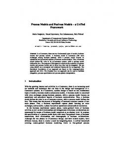
VI. EXAMPLESAND DISCUSSIONS In this section, we provide an example, based on a model of a computing system, to illustrate the effectiveness of the different variance reduction techniques discussed in the previous sections. A block diagram of the computing system considered is shown in Fig. 1. We use two different parameter sets to create a “balanced and an “unbalanced” system. A balanced system is one in which each type of component has the same amount of redundancy, (i.e., same number of components of a type must fail in order that the system fail, e.g., 1-out-of-2 of a type has the same redundancy as 3-outof-4 of another type); in addition, the components must have

45

processors

cc

Fig. 1 A block diagram of the computing system modeled.

the same order of magnitude failure rates. A system that is not balanced is unbalanced. For a balanced system we select two sets of processors with two processors per set, two sets of controllers with two controllers per set, and six clusters of disks, each consisting of four disk units. In a disk cluster, data are replicated so that one disk can fail without affecting the system. The “primary” data on a disk is replicated such that one third is on each of the other three disks in the same cluster. Thus, one disk in each cluster can be inaccessible without losing access to the data. The connectivity of the system is shown in Fig. 1. We assume that when a processor of a given type fails, it has a 0.01 probability of causing the operating processor of the other type to fail. Each unit in the system has two failure modes which occur with equal probability. The failure rates of processors, controllers, and disks are assumed to be 1/2000, 1/2000, and U6000 per hour, respectively. The repair rates for all mode 1 and all mode 2 failures are 1 per hour and 1/2 per hour, respectively. Components are repaired by a single repairman who chooses components at random from the set of failed units. The system is defined to be operational if all data are accessible to both processor types, which means that at least one processor of each type, one controller in each set, and 3 out of 4 disk units in each of the 6 disk clusters are operational. We also assume that operational components continue to fail at the given rates when the system is failed. We make minor changes to the above parameters setting in order to create an unbalanced system. We increase the number of processors of each type to 4, and double each processor’s failure rate to 1/1000 per hour. We decrease the failure rates of all other components by a factor of ten. In this system, although a processor failure is more likely to occur in a failure transition, it is less likely to cause a system failure due to the high processor redundancy. This is typical behavior for an unbalanced system.

A. Steady-State Measures In this section we discuss the results of our experiments for estimating the steady-state unavailability and the mean time to failure. Numerical (nonsimulation) results for these measures were obtained using the SAVE package [18]. Since


46

the balanced system has a few hundred thousand states and the unbalanced system has close to a million states, only bounds could be computed ([35]). These bounds are very tight and typically do not differ from the exact results significantly. We simulate both the balanced and the unbalanced systems. The goal of the simulation experiments is to study the efficiency of the importance sampling methods, described in this paper, compared to standard simulation. We also experimented with the MSDIS technique described in Section 111. It is shown that the Bias1 method gives many orders of magnitude variance reduction over the standard Monte Carlo simulation. Moreover, further significant improvements can be obtained using the BiasllBias2 method for the balanced systems and BiasllBalancing method for the unbalanced systems. Further improvements are obtained when these methods are combined with MSDIS. Table I and Table I1 show the results obtained for the balanced and the unbalanced systems, respectively. We ran the simulation long enough so that the smallest entry in the tables for the percentage relative half-widths of the 90% confidence intervals was less than 5%. The percentage relative half-width of a confidence interval is defined to be 100% times the confidence interval half-width divided by the point estimate. This corresponds to approximately 100 000 events for each entry in Table I and 1 000 000 events for each entry in Table 11, respectively. For the MSDIS entries, we assigned 10% of the total events to estimate the denominator (numerator) for unavailability (MTTF) as suggested in Section 111-D. Based on empirical results obtained in [4], [19], and [43], the values for bias1 and bias2 were selected as follows: for DIS, 0.5 and 0.5, and for MSDIS, 0.9 and 0.9. For the balanced system (Table I), the BiasllBias2 method is most effective, which supports our intuition that it helps push the system quickly toward a likely path to failure. For the unbalanced system (Table 11), the BiasllBaZancing is the most effective method, which also supports our intuition as follows. By making individual failures equally likely we are also increasing the failure probability of a more reliable but less redundant component, thus leading to a more likely path to failure. Note that the percentage relative half-widths for both the steady-state unavailability ( U ) and the mean time to failure (MTTF) are approximately equal. This is because the estimate of U is approximately proportional to the estimate of l/MT"F. To see this, using the notation of Section 11, m i n ( a F , (YO) = QO with high probability when no importance sampling is used. Thus an individual sample r.v. in the numerator of the ratio for MTTF (2.9) is equal to the r.v. in the denominator of U (2.7) with high probability. Now for the three state model, a sample r.v. G in the numerator of U is G = h2 x n F where n F is the number of times the failure state is entered. Using our importance sampling schemes, G = h 2 l i n F Z l )with high with high probability. Furthermore, l{nF=l} = 1{,,,,,) probability so an individual sample r.v. in the denominator of the M'ITF ratio is proportional to the r.v. in the numerator of U with high probability. Thus, an estimate of U is approximately proportional to 1°F. Finally, direct manipulation of the asymptotic variance (3.6) shows that the relative half-width of a ratio is equal to the relative half width of its reciprocal.


We next performed the coverage experiments (see e.g., [26]) to determine the validity of the confidence intervals that are formed based on the asymptotic central limit theorems described in Section 111. Such studies are important since certain variance reduction techniques sometimes do not produce valid confidence intervals, except for very long run-lengths (see e.g., [26]). In such cases, the variance reduction technique cannot be relied upon to actually shorten simulation run lengths. We performed coverage experiments on estimates of the steadystate unavailability, U , in the above described balanced system as follows. We chose three run lengths corresponding to small, medium and large sample sizes and considered three ways of estimating U : standard simulation, the BiasllBias2 method with DIS and the BiasllBias2 method with MSDIS. For each method and run length we ran R = 100 replications and formed point estimates U,, ' . ' , U, and 90% confidence intervals. We then calculated the mean percent relative bias (= 100% x ( l / R ) xkl(Ui- U ) / U ) and the standard deviation of this mean. Note that if an estimate is unbiased, then its mean percent relative bias should converge to zero as R + CO. We also calculated the 90% coverage which is the percentage of the (alleged) 90% confidence that actually contain the true value U. If the confidence interval is valid, then by definition, the 90% coverage should be close to 90%. We also computed the mean percent relative half width of the 90% confidence intervals. For each replication, this relative value is computed using the point estimate and not the true value. The mean is computed over all replications with a nonzero point estimate. The results are listed in Table 111. As anticipated from Section 111-E, the standard estimate is significantly more biased than either the DIS-BiasllBiasZ or the MSDIS-Biasl/Bias2 estimates and that its confidence intervals are at least an order of magnitude wider. Furthermore, for the small run length, its coverage drops significantly below 90%. In fact, there were no system failures in the runs corresponding to the 46% of the confidence intervals which did not contain U . Using our variance reduction techniques, all the coverages are close to the nominal 90% value except for the longest run using MSDIS which had a coverage of 81%. Changing the random number generator from the multiplicative linear congruential generator In+l = ( I , x 16807) mod 231 - 1 to the combined generator described in [27], and running R = 200 replications, increased the coverage to 85% which still represents a statistically significant departure from 90%. Despite a considerable effort, we have been unable to identify the source of this slight coverage problem. However, note that the first nonzero digit in U is in the sixth decimal place, so the problem (if any) is occurring in the eighth decimal place. In practice, such high precision may not be warranted, given inaccuracies in model parameters and distributional assumptions.

B. Transient Measures In this section we discuss the results of our experiments for estimating reliability and expected interval availability. Recall that for transient measures we not only want the system to move quickly toward the set of system failed states F ,


47


Numerical Results

Direct

10.9309x

1.0171 x

(0.5)

(0.5)

(0.5/0.5)

MSBias 1/Bias2 (0.9/0.9)

0.9779 x

0.9547 x lo-'

0.9395 x lo-'

0.9317 x

Bias 1

Biasl/Balancing Biasl/Bias2

Unavailability f 27.1 YO

f 7.6 Yo

f 6.2 Yo

& 2.7 Yo

* 1.0 Yo

0.1637 x

0.1524 x

0.1581 x lof6

0.1631 x lof6

0.1626 x lof6

0.1633 x lof6

MTTF

- 25.7 Yo

+

f 7.0 Yo

f 5.7 Yo

*

f 1.0 Yo

Numerical Results

Direct

Bias 1

Biasl/Balancing Biasl/Bias2

(0.5)

(0.5)

(0.5/0.5)

MSBias 1/Balancing (0.9)

0.6967 x

0.4164 x lo-'

0.6644 x

0.6976 x

0.6375 x lo-'

0.6810 x

Unavailability

164.5 YO

2.5 %

f 46.1 YO

f 2.4 Yo

f 5.6 Yo

f 2.2 Yo

0.2188 x 10"

0.4703 x 10"

0.2227 x lo+'

0.2183 x lo+'

0.2349 x lo+'

0.2222 x 10"

MTTF

f 164.5 Yo

+ 43.7 Yo

f 2.3 Yo

f 5.1 Yo

f 2.0 Yo

TABLE I11 COVERAGE EXPERIMENTS FOR THE BALANCED SYSTEM Events per Replication

MS - Biasl/Bias2 (0.9/0.9)

Direct Simulation

BiasliBias.2 (0.5/0.5) Relative H W

Coverage

Relative Bias (Std. Dev.)

Relative HW

Coverage

(Std. Dev.)

Relative Bias (Std. Dev.)

2000

6.95 Yo (12.88 Yo)

0.74 Yo (1.21 Yo)

18.88 Yo

85 %

0.35 Yo (0.91 Yo)

6.70 Yo

91 %

20000

-3.94 %

0.39 % (0.34 Yo)

5.99 Yo

90 Yo

0.11 Yo (0.22 Yo)

2.56 Yo

91 %

200000

1.29 Yo (1.09 Yo)

0.05 Yo (0.13 Yo)

1.90 Yo

90 Yo

0.03 Yo (0.073 Yo)

1.04 YQ

81 Yo

19.6 Yo

96 Yo

but also reach there before the observation period expires. Since these two issues are, in some sense, orthogonal, we use the same technique as in the steady-state case to bias the embedded Markov chain toward the system failed set, in addition to another independent technique (e.g., forcing or conditioning as discussed in Section V) to reduce the variance due to holding times in the various states. The likelihood ratios corresponding to these two aspects of simulation are independent and can be formulated as in Proposition 4.1. The goal of the simulation is to study the effect of the forcing and conditioning techniques. We considered only the balanced system. For each measure, we allowed each method to run for 400 000 events. Standard simulation was not considered as it is very ineffective for estimating transient measures. The results are given in Tables IV and V.

For all methods, the confidence intervals are smaller for some range of intermediate time periods and wider at the ends. To explain this, we recognize two key factors affecting the variance of the estimates; namely, the number of replications in a simulation run and the value of biusl used with importance sampling. For smaller time intervals, there are more replications in a simulation run than for larger time intervals (since we kept the total number of events fixed). This contributes to a larger variance for larger time intervals. Furthermore, for each time interval, there is an optimal value for biusl which maximizes the variance reduction. While bias1 = 0.5 may be close to optimal for some intermediate range of time intervals, it departs from the optimal value for either smaller or larger time intervals. The two tables indicate that forcing and conditioning are



48

TABLE IV UNRELIABILITY ESTIMATES IN A BALANCED SYSTEM

Time (r) Vumencal in Jnreliability Hours 4

-t

Biasl ( O S ) Standard

f 25.0 Yo f

16

3ias 1/Bias2

Bias 1/Balancing (0.5) Forcing

Conditioning Standard

,1477

.1435

5.2 Yo ,8569 x

1 0 - ~ ,1255

lo4

.I531

.5/o.5)

Conditioning jtandard

Forcing io4

,1463

1583

lo4

f 7.5 Yo

f 21.3 Yo

f 4.0 ‘?A

f 5.5 %

t 7.0 Yo

,8383 x lo4

,8855x lo4

,8565 x IO“

,8301 x

8693 x

k 3.3 Yo

f 10.7 Yo

3801 x

64

k 1.8 Yo 1565 x

256

1024

+ 5.8 YQ

k 1.5 Yo

1.1968 x IO-

6275 x

I 6226 x

++ +

k 4.9

f 73.3 Yo

-

TABLE V EXPECTED INTERVAL UNAVAILABILITY ESTIMATES IN A BALANCED SYSTEM

rime ( t n Hours

Vumerical

1

3178 x lo-’

Forcing

1024

,2572 x lop5

f 6.8 Yo

f 4.7 Yo

f 27.5 %

7148

,7401 x lo-’

,7677 x

k 6.7 %

f 3.9 Yo

f 12.9 a?‘

f 5.5 %

f 3.1 Yo

f 4.8 Yo

* 2.1

,8651 x lo-’

,9012 x

,8822 x IO-’

,8862 x IO-’

,8966 1 0 - ~ ,8821

f 3.2 Yo

+

56 9178 x

Conditioning Standard

,3057 x lop5 3110 x 1 0 - ~ ,3224 x

f 15.8 %

54

I Bias 1/ Bias2 (0.5/0.5)

IBias 1/Balancing (0.5)

Biasl (0.5)

Interval Unavailability

f 3.5.0 Yo

16

To

8866 x l o r 5 .9276 x IO-’

%

f 1.2 Yo

lo-’

f 11.4 %

k 8.3 %

f 6.6 Yo

f 4.0 %

f 2.4 Yo

f 1.5 Yo

.9882 x

9442

1.0766 x

1.0010 x lo-’ .9049 x

,9133 IO-’

,9063

k 12.9 Yo

f 13.9 Yo

f 9.3 Yo

f 4.4 Yo

f 4.2 Yo

f 3.3 Yo

9677 x l o r 5

.3707 x IO-’

.6168 x lo-’

1.0760 x 10- 1.0728 x IO-’ .7822 x

f 36.1 %

f 51.6 Yo

f 64.8 Yo

If

91.5 %

lo-’

t 91.5 Yo

& 103.5 Yo

If

36.3 %

most effective for short time intervals. This is intuitive because for a long interval enough transitions occur before the interval expires, and therefore, the embedded Markov chain has a chance to reach the system failed set using only failure biasing. This is not true for short intervals, and therefore, either forcing transitions to occur before the end of the period or conditioning the holding time out in state 0 has a significant effect. Both forcing and conditioning give similar results for unreliability, while conditioning is consistently better for the interval unavailability. Note that for interval unavailability we are using (4.7) with conditioning, but not with forcing. However, forcing can be similarly combined with (4.7) to possibly yield better results. Also, note that

f 65.0 Yo

IO-^

f 21.3 Yo

BiasllBias2 method is consistently better than both the Biasl and the BiasllBalancing methods. This is consistent with a similar conclusion with respect to the steady-state measures in a balanced system.

VII. SUMMARY AND DIRECTIONS FOR FUTURE WORK In this paper, we have developed a unified framework for simulation of Markovian models of highly dependable systems. Conventional numerical techniques are difficult to apply to this class of stochastic models because of the fact that the size of the state space of the Markovian model increases exponentially with the number of components in the system.



On the other hand, simulation algorithms tend to be relatively insensitive to the size of the state space of the simulated Markovian model, both in terms of storage and computational requirements. However, standard simulation is inefficient in our setting because the principle focus of interest; namely, system failures, occur so infrequently in highly dependable systems. As a consequence, few system failures, if any, would be observed if standard simulation methods were to be used in our problem context. The emphasis in this paper has therefore centered on applying variance reduction techniques to improve the efficiency of the simulations associated with Markovian models of highly dependable systems. We have reviewed the basic theory of importance sampling in several elementary problem settings and then used this insight to develop sampling heuristics for the complex systems of interest here. Different variants of these ideas were developed for both transient and steadystate dependability measures. In addition, we have "fine-tuned" the importance sampling techniques to take advantage of the structure of highly dependable systems which are either balanced or unbalanced. Our work has also shown that importance sampling may be fruitfully applied in conjunction with a variance reduction method known as conditioning. The basic idea here was to observe that highly dependable systems spend a significant fraction of time in the state in which all components are fully operational. Since the stochastic behavior of the time spent in the fully operational state was easy to calculate analytically, this permitted us to effectively integrate out the randomness in our importance sampling estimators due to the holding times in the fully operational state. Our empirical investigation showed that the combined variance reduction obtained by using both conditioning and importance sampling is typically substantial. In fact, in all of our experiments, our methods yielded estimators in which the variance was decreased by several orders of magnitude. In a recent analytical work in this area ([44]), the heuristics used in this paper have been proven to be very efficient. Our empirical work also showed that the confidence intervals associated with our estimators typically provided acceptable levels of coverage. We view this as important, since the scientific representation of the accuracy of a simulation estimator is usually gauged through a confidence interval. A number of possible directions for future research present themselves. One important issue relates to the fact that the importance sampling heuristics presented in this paper were basically developed for systems in which system dependability is achieved principally through high component reliability. However, another approach to obtaining high system dependability is through high levels of component redundancy. Importance sampling methods approprizte for the analysis of highly redundant systems differ from those presented here. Such techniques would likely have important ramifications for the simulation of certain highly dependable systems. A second important research area involves the generalization of the ideas developed in this paper to stochastic models of highly systems in which the underlying failure . dependable . and repair distributions are nonexponential. Since the resulting

49

stochastic process is typically no longer either Markovian or regenerative, many of the ideas presented in this paper cannot be implemented directly. Some work in this direction is reported in [37]. APPENDIX ESTIMATING THE DISTRIBUTION OF INTERVAL AVAILABILITY We will find it more convenient to estimate the distribution of the time in the set of failure states, U ( t ,x) = P { U ( t )I z}, where U ( t ) = Jstt=o l { Y s E F ) d ~Since . A ( t ) = 1 - U ( t ) / t we have A ( t , x ) = P { A ( t ) I x} = 1 - U ( t ,(1 - z ) t ) .To derive an estimator for U ( t , x ) ,write

U ( t ,x) = Ul(t, x) + UZ(t, ).

(A.1)

where Ul(t,x) = P{U(t) 5 x , y t F } and U~(t,x) = P{U(t) I x,K E F}. Define D, = xi=ot31{~,E~} and

C, = t,l{x,+o,x,g~}, with Y,,4, and no(i) as defined previously. Note that 4, = C, D, and T,+1 = y, C, D,. Consider U1(t, x):

+ +

+

U1(t,x) = P { U ( t ) I x,yt

# F}

00

=

P{U(t)

I x,X,# F,N ( t ) = i}

2=0 00

= CP{D,-i

5 x , X , # F,T, < t < Tz+1}

2=0

2=0

+ 42-1

< t < Yz + 42).

(A.2)

Now if X, = 0, then dzP1= 4,.If X,# F and X, # 0, then no(z - 1) = no(z) and therefore yz-l = 7,. In either case, by conditioning on the sequence of states and the holding times in the nonzero states, we can write Ul(t,X) = E

[

03

l { D , - l < z , x , @ F }(Eno(z-l)(t - 4 2 - 1 ,

Xo)

2=0

- Eno(z)(t- 4 2 , Xo))

1

.

('4.3)

Now consider UZ(t,x). If Yt E F and N ( t ) = a, then U ( t ) = DZp1 + t - T, = t - -y,-l - Cz-l. Furthermore, on this set no(z - 1) = no(z),yz-l = y, and C,-l = C, so that 0

0

,

-



50

This development provides a computationally attractive way to estimate U ( t ,x) without sampling from the state 0 holding time distribution. It is easily combined with failure biasing. Practical implementations may require truncation or stopping rules as described in Section IV-B.

REFERENCES [I] A. Bobbio and K. S. Trivedi, “An aggregation technique for the transient analysis of stiff Markov chains,” IEEE Trans. Comput., vol. C-35, pp. 803-814, 1986. 12) W. G. Bouricius, W. C. Carter, and P. R. Schneider, “Reliability modeling techniques for self-repairing computer systems,” in Proc. ACM Nat. Conj, San Francisco, CA, 1969, pp. 295-309. [3] K. L. Chung, Markov Chains With Stationary Transition Probabilities, Second Edition. New York: Springer-Verlag, 1967. [4] A. E. Conway and A. Goyal, “Monte Carlo simulation of computer system availability/reliability models,” in Proc. Seventeenth Symp. FaultTolerant Comput., Pittsburgh, PA, 1987, pp. 230-235. [5] A. Costes, J. E. Doucet, C. Landrault, and J. C. Laprie, “SURF-A program for dependability evaluation of complex fault-tolerant computing systems,” in Proc. Eleventh Symp. Fault-Tolerant Comput., Portland, ME, 1981, pp. 72-78. [6] M. Cottrell, J. C. Fort, and G. Malgouyres, “Large deviations and rare events in the study of stochastic algorithms,” IEEE Trans. Automat. Contr., vol. AC-28, pp. 907-920, 1983. [7] H. CramCr, Mathematical Methods of Statistics. Princeton, NJ: Princeton University Press, 1946. [8] M. A. Crane and D. L. Iglehart, “Simulating stable stochastic systems, 111: Regenerative processes and discrete event simulations,” Oper. Res., vol. 23, no. 1, pp. 3 3 4 5 , 1975. [9] J. B. Dugan, K. S. Trivedi, M. K. Smotherman, and R.M. Geist, “The hybrid automated reliability predictor,” J. Guidance, Contr., Dynamics vol. 9, no. 3, pp. 319-331, 1986. [lo] B. L. Fox and P. W. Glynn, “Discrete-time conversion for simulating semi-Markov processes,” Oper. Res. Lett., vol. 5, pp. 191-196, 1986. [ 1I] -, “Discrete-time conversion for finite-horizon Markov processes,” SIAM J. Appl. Math., vol. 5, no. 5, pp. 1457-1473, 1990. [12] R. M. Geist and K. S. Trivedi, “Ultra-high reliability prediction for fault-tolerant computer systems,” IEEE Trans. Comput., vol. C-32, pp. 1118-1127, 1983. [13] R. M. Geist and M. K. Smotherman, “Ultrahigh reliability estimates through simulation,” in Proc. Annu. Reliability and Maintainability Symp., Atlanta, GA, 1989, pp. 350-355. [14] P. W. Glynn and P. Heidelberger, “Bias properties of budget constrained simulations,” Oper. Res., vol. 38, no. 5, pp. 801-814, 1990. [15] P. W. Glynn and D. L. Iglehart, “Importance sampling for stochastic simulations,” Management Sci., vol. 35, no. 11, pp. 1367-1392, 1989. [16] A. Goyal, W. C. Carter, E, de Souza e Silva, S. S. Lavenberg, and K. S. Trivedi, “The system availability estimator,” in Proc. Sixteenth Symp. Fault-Tolerant Comput., Vienna, Austria, 1986, pp. 84-89. [I71 A. Goyal, S. S. Lavenberg, and K. S. Trivedi, “Probabilistic modeling of computer system availability,” Ann. Oper. Res., vol. 8, pp. 285-306, 1987. [18] A. Goyal and S.S. Lavenberg, “Modelihg and analysis of computer system availability,” IBM J. Res. Develop., vol. 31, pp. 651-664, 1987. [19] A. Goyal, P. Heidelberger, and P. Shahabuddin, “Measure specific dynamic importance sampling for availability simulations,” in I987 Winter Simulation Conj Proc., A. Thesen, H. Grant, and W.D. Kelton, Eds., IEEE Press, 1987, pp. 351-357. 1201 D. Gross and D. R. Miller, “The randomization technique as a modeling tool and solution procedure for transient Markov processes,” Oper. Res., vol. 32, pp. 343-361, 1984. J. M. Hammersley and D. C. Handscomb, Monte Carlo Methods. London, England: Methuen, 1964. A. Hordijk, D. L. Iglehart, and R. Schassberger, “Discrete time methods for simulating continuous time Markov chains,” Adv. Appl. Prob., vol. 8, pp. 772-788, 1976. H. Kahn and A. W. Marshall, “Methods of reducing sample size in Monte Carlo computations,” J. Oper. Res. Soc. Amer., vol. 1, no. 5, pp. 263-278, 1953. S. Karlin and H. M. Taylor, A First Course in Stochastic Processes, Second Edition. New York Academic, 1975. [25] D. E. Knuth, “Big omicron, big omega and big theta,” SIGACT News (ACM), vol. 8 , no. 2, pp. 18-24, 1976.

[26] S. S. Lavenberg, T. L. Moeller, and C. H. Sauer, “Concomitant control variables applied to the regenerative simulation of queueing systems,” Oper. Res. vol. 27, no. 1, pp. 134-160, 1979. I271 P. L’Ecuyer, “Efficient and portable combined random number generators,” Commun. ACM, vol. 31, no. 6, pp. 742-774. 1988. [28] E. L. Lehmann, Theory ofpoint Estimation. New York: Wiley, 1983. [29] E. E. Lewis and F. Bohm, “Monte Carlo simulation of Markov unreliability models,” Nuclear Eng. and Design, vol. 77, pp. 49-62, 1984. [30] C. A. Liceaga and D. P. Siewiorek, “Toward automatic Markov reliability modelling of computer architectures,” NASA Tech. Memo. 89009, 1986. [31] S.V. Makam, A. Avizienis, and G. Grusas, UCLA ARIES 82 User’s Guide. Also Tech. Rep. CSD-820830, Univ. of California at Los Angeles, 1982. [32] A.M. Johnson, Jr. and M. Malek, “Survey of software tools for evaluating reliability, availability, and serviceability,” ACM Comput. Surveys, vol. 20, no. 4, pp. 227-269, 1988. [33] J. F. Meyer, “On evaluating the performability of degradable computing systems,” IEEE Trans. Comput., vol. C-29, no. 8, pp. 720-731, 1980. [34] R. G. Miller, “The Jackknife-A review,” Biometrika, vol. 61, pp. 1-15, 1974. [35] R. R. Muntz, E. de Souza e Silva, and A. Goyal, “Bounding availability of repairable computer systems,” IEEE Trans. Comput., vol. 38, no. 12, pp. 1714-1723, 1989. [36] V. F. Nicola, “Lumping in Markov reward processes,” IBM Res. Rep. RC 14719, Yorktown Heights, N?’, 1989. [37] V.F. Nicola, M.K. Nakayama, P. Heidelberger, and A. Goyal, “Fast simulation of dependability models with general failure, repair and maintenance processes,” in Proc. Twentieth Symp. Fault-Tolerant Comput., Newcastle upon Tyne, England, 1990, pp. 491498. [38] S. M. Ross, Applied Probability Models with Optimization Applications. San Francisco, CA. Holden-Day, 1970. [39] S. M. Ross and Z. Schechner, “Using simulation to estimate first passage distribution,” Management Sci., vol. 31, no. 2, pp. 224-234, 1985. [40] S. Parekh and J. Walrand, “A quick simulation method for excessive backlogs in networks of queues,” IEEE Trans. Automat. Contr., vol. 34, no. 1, pp. 54-66, 1989. [41] R. A. Sahner and K. S. Trivedi, “Performance and reliability analysis using acyclic directed graphs,” IEEE Trans. Sofhvare Eng., vol. SE-13, no. 10, pp. 1105-1114, 1987. [42] W. H. Sanders and J. F. Meyer, “METASAN: A performability evaluation tool based on stochastic activity networks,” in Proc. 1986Fall Joint Comput. Con$, AFIPS, NY, 1986, pp. 807-816. (431 P. Shahabuddin, V. F. Nicola, P. Heidelberger, A. Goyal, and P. W. Glynn, “Variance reduction in mean time to failure simulations,” in I988 Winter Simulation Conj Proc., M. A. Abrams, P. L. Haigh, and J.C. Comfort, Eds., IEEE Press, 1988, pp. 491-499. [44] P. Shahabuddin, “Simulation and analysis of highly reliable systems,” Ph.D. dissertation, Dep. Oper. Res., Stanford Univ., 1990. [45] D. Siegmund, “Importance sampling in the Monte Carlo study of sequential tests,” Ann. Statistics, vol. 4, pp. 673484, 1976. [46] W. L. Smith, “Regenerative stochastic processes,” Proc. Roy. Soc. A., vol. 232, pp. 6-31, 1955. 1471 J. Walrand, “Quick simulation of rare events in queueing networks,” in Proc. Second Int. WorkshopAppl. Math. and PerformancelReliabiIity Models of ComputKommun. Syst., G. Iazeolla, P. J. Courtois, and 0 .J. Boxma, Eds. Amsterdam, North Holland, 1987, pp. 275-286.

I

Ambuj Goyal (S’81-M’82) received the B.Tech. degree from the Indian Institute of Technology, Kanpur, and the M.S. and Ph.D. degrees from the University of Texas at Austin, He is a research staff member at the IBM Thomas J. Watson Research Center where he manages the Fault-Tolerant Systems Theory group. His research interests include fault-tolerant computing, computer architecture, communication networks, and performance evaluation. Dr. Goyal is a member of the IEEE Computer Society. He has served as the Program Committee Chairman of the Workshop on Reliability/Availability Modeling Tools and Their Applications.



Penvez Shahabuddin received the B.Tech. degree in mechanical engineering from the Indian Institute of Technology, Delhi, in 1984. After working for a year in Engineers India Limited, India, he joined the Ph.D. program in Operations Research at Stanford University, Stanford, CA. After completing the Ph.D. degree in 1990, he joined the IBM T. J. Watson Research Center as a Research Staff Member. His research interests include simulation techniques, queueing theory, and performance analysis of computer systems. Dr. Shahabuddin is a member of the Operations Research Society of America.

Philip Heidelberger (M’82) received the B.A. degree in mathematics from Oberlin College, Oberlin, OH, in 1974 and the Ph.D. degree in operations research from Stanford University, Stanford, CA, in 1978. He has been a Research Staff Member at the IBM Thomas J. Watson Research Center, Yorktown Heights, NY, since 1978. His research interests include modeling and analysis of computer performance and statistical analysis of simulation output. Dr. Heidelberger is an Associate Editor of Operations Research and was the Program Chairman of the 1989 Winter Simulation Conference, which is co-sponsored by the IEEE. He is a member of the Operations Research Society of America and the Association for Computing Machinery.

51

Victor F. Nicola (M’89) received the B.S. and M.S. degrees in electrical engineering from Cairo University, Egypt, and Eindhoven University of Technology, The Netherlands, respectively, and the Ph.D. degree in computer science from Duke University, Durham, NC, in 1986. In 1979 he joined the scientific staff of the Measurement and Control Group at Eindhoven University. Currently, he is a Research Staff Member with the Department of Computer Sciences at IBM Thomas J. Watson Research Center. His research interests include perf01rmance and reliability modeling of computer systems, queueing theory, fault tolerance, and simulation. Dr. Nicola is a meniber of the IEEE Computer Society.

Peter W. Glynn received the Ph.D. degree from Stanford University, Stanford, CA, in 1982. He spent five years as an Assistant Professor in the Department of Industrial Engineering at the University of Wisconsin-Madison. He is currently an Associate Professor in the Department of Operations Research at Stanford University. His research interests include stochastic systems, computational probability, and simulation.


A unified framework for simulating Markovian models ...

A unified framework for simulating Markovian models ...

Suggest Documents

A unified framework for differential aggregations in Markovian process ...

StarL: Towards a Unified Framework for Programming, Simulating and ...

A Unified Theoretical Framework for Mapping Models for the

A unified theoretical framework for fluctuating-charge models in ... - arXiv

Markovian Models for Sequential Data

a Unified Framework - CiteSeerX

Simulating The Republican âUnified Framework ... - Laurence Kotlikoff

A framework for modeling and simulating energy

Markovian Framework for Foreground-Background-Shadow ...

A UNIFIED FRAMEWORK FOR GENERALIZED MULTICATEGORIES

A Framework for the Unified Presentation of

Relativization a Framework for Constructing Unified ...

A Unified Framework for Probabilistic Component Analysis

A unified geometric framework for the statistical

A Unified Computational and Statistical Framework for

A Unified Framework for Adaptive BDDC - Ricam

Towards A Novel Unified Framework for Developing

A Unified Framework for Bases, Frames, Subspace

A Unified Authentication Framework for JPEG2000

Understanding Forecasting: A Unified framework for ...

A Unified Conceptual Framework for Service ...

A unified framework for non-Brownian suspension

A Unified Framework for Adaptive BDDC - Ricam

A Unified Security Framework for Networked Applications

A unified framework for simulating Markovian models ...