408
IEEE TRANSACTIONS ON SYSTEMS, MAN, AND CYBERNETICS—PART A: SYSTEMS AND HUMANS, VOL. 28, NO. 4, JULY 1998
A Unified Model for Abduction-Based Reasoning B´echir Ayeb, Member, IEEE, Shengrui Wang, and Jifeng Ge
Abstract— In the last decade, abduction has been a very active research area. This has resulted in a variety of models mechanizing abduction, namely within a probabilistic or logical framework. Recently, a few abductive models have been proposed within a neural framework. Unfortunately, these neural/probablistic-/logical-based models cannot address complex abduction problems. In this paper, we propose a new extended neural-based model to deal with abduction problems which could be monotonic, open, and incompatible. Index Terms— Competition model, distributed processing, monotonic/open/incompatibility abduction problems, neural networks.
I. PROLOGUE
T
HE intuition behind abduction can be stated as follows [5], [31]. Given an observation (e.g., a manifestation or a symptom in medicine), a hypothesis (e.g., a disorder or a disease in medicine), and the knowledge that causes , it is an abduction to hypothesize that occurred. The main issue of abduction is to synthesize a composite hypothesis explaining the entire observation from elementary hypotheses. In [5], deep insights into the mechanization of abduction were pointed out. The computational complexity of each class of abduction problems has been provided. In fact, the ubiquity of abduction is remarkable. Once one learns it, one discovers it virtually everywhere. This includes diverse areas such as diagnosis [34], planning [17], natural language processing [7], machine learning [28], legal reasoning [41], and text processing [27]. Unfortunately, the applicability of abduction suffers from its computational complexity. Although abduction is in general NP-Hard [5], [18], some models (e.g., [1], [2], [4], [9], [25], [29], [32], [35]) aiming at mechanization of abductive reasoning (called also hypothetical reasoning) have been provided. All of these models make several assumptions to address only a simple case, called the class of independent abduction problems. The main objective of this paper is to address complex classes of abduction. Specifically, we propose a unified neuralbased model dealing with the monotonic class, the open class, and the incompatibility class of abduction problems. The strengths of this work are two-fold. First, it is innovative. Manuscript received November 7, 1995; revised October 15, 1996 and October 22, 1997. This research was supported in part by the NdL project under FRAI Grants 0238A and 0291A and NSERC Grants OGP0121468/OGP0121680; EQP0121469/EQP0139397. Project ?dL/NdL is an experimental diagnosis laboratory which aims at adapting and mechanizing model-based diagnosis techniques depending on the class of diagnostic problems. The authors are with the Faculty of Sciences/DMI, University of Sherbrooke, Sherbrooke, P.Q., Canada J1K 2R1 (e-mail:
[email protected];
[email protected];
[email protected]). Publisher Item Identifier S 1083-4427(98)04360-4.
To our knowledge, this is the first model which tackles complex abductive problems (e.g., the incompatibility class) and provides an effective algorithm to generate explanations for this class. Second, it is instructive in itself. Starting from a simple model addressing the class of independent abduction problems, we extend progressively this model to address a variety of abduction problems regardless of their class. Consequently, we show how neural networks can be very effective to address complex problems. We also open the door for a wide applicability of abduction on real-world problems. The rest of this paper is organized as follows. Section II gives preliminary material on abduction. Section III presents our initial model for the independent class. Section IV provides in a stepwise refinement way our unified model. Section V summarizes our model and theoretical foundations. Section VI discusses related work and experimental results. Section VII includes concluding remarks and further research. II. CONCISE SUMMARY ON ABDUCTION CLASSES The main goal of this section is to provide preliminary materials on abduction, facilitate the introduction of neuralbased abduction, and characterize in a concise way different classes of abduction problems.1 Depending on the context, an abduction problem can be formalized in several ways. Let us adopt the following definition. Definition 1: An abduction problem AP is a tuple , where and are two disjoint finite sets of is a finite set of causal relationships between symbols; and . Intuitively, denotes the set of elementary hypotheses, denotes the set of observable facts, whereas denotes to . Following the form of the causal a mapping from relationships embedded in , we can introduce several classes of abduction problems. For convenience, let us first introduce the following notation. , a subset of elementary hyNotation 1: Consider , an observable fact. We write potheses and to express a causal relationship between the hypotheses in and the observable fact with a given weight [0, 1]. In the following, we say that is covered by with respect may cause with the weight . to a weight , or A. Independent and Monotonic Abduction Problems Using Notation 1, we now define straightforwardly the class of independent and monotonic abduction problems. 1 For a thorough and general introduction to abduction, see [5], [33], and [37].
1083–4427/98$10.00 1998 IEEE
AYEB et al.: UNIFIED MODEL FOR ABDUCTION-BASED REASONING
Fig. 1. A general abduction problem.
Definition 2: Let be an abduction problem, then we have the following. AP belongs to the independent class if each causal relacan be expressed as , where tionship in and . In other words, each causal relationship involves exactly one and only one elementary hypothesis and one observable fact. Hence, there is no interaction between the elementary hypotheses in . AP belongs to the monotonic class if there is at least one which is expressed as: , causal relationship in and does not hold. This time, where an additive interaction between the hypotheses in is required to cause the observable fact . Fig. 1 introduces a general abduction problem2 , where parenthesized identifiers refer , let us define , an to abbreviated names. Using , a monotonic independent abduction problem, and abduction problem, as follows. , where Example 1: , and . where Example 2: , and . 2 This is drawn from mechanical engineering, namely an oversimplified model for automobile troubleshooting [8]. We do not intend that our illustrative examples correspond to actual cases; real-world cases are reported in Section V. Note also that weights of causal relationships are split into several categories, e.g., weight 1.0 (resp., 0.75, 0.5) expresses must cause, (resp., may cause, leads to) relationships. Other categories could be introduced depending on the application domain.
409
Given an abduction problem, we introduce the concept of a simple observation as follows. be an independent or a Definition 3: Let monotonic abduction problem, a simple observation SO is a . given subset of observed facts, SO As an example, let us consider the following simple observations. Example 1 (Continued): SO . Example 2 (Continued): SO . The following notation, inspired from [5], [33], is useful to introduce the concept of explanation for an abduction problem. be an elementary hypothesis and Notation 2: Let causes , i.e., . We suppose that . define the following “function”: EXPLAIN denotes a subset of elementary hypotheses, then If EXPLAIN . EXPLAIN Definition 4: Let be an independent or a monotonic abduction problem. Suppose that SO is a given , then an explanation for simple observation for with respect to SO is such that: 1) , 2) SO EXPLAIN , and 3) is minimal with respect to set has the inclusion/cardinality. If among all explanations, maximal plausibility (i.e., with respect to a given belief is said to be the best explanation. function) then For our illustrative examples, we have the following explanations. , Example 1 (Continued): for with respect and to SO . , Example 2 (Continued): for with respect and to SO . Notice that the above explanations take minimality criterion and appear to with respect to set cardinality. Moreover, be the best explanations if plausibility is a simple normalized sum of weights attached to causal relationships. B. Open and Incompatibility Abduction Problems Unlike independent and monotonic classes, open and incompatibility classes require introduction of the concept of multiple observation as follows. be an abduction problem, Definition 5: Let where a multiple observation MO is an uplet denotes the facts which are known to be present, denotes the facts which are known to be absent, denotes the unknown facts. Naturally, we have and . Now, we introduce a final convention followed by two definitions related to the class of open and incompatibility abduction problems. Notation 3: We make use of the distinguished symbol to denote a fact which can never be observed. Definition 6: Let be an abduction problem. is necessarily multiple, Suppose that every observation to then we have:
410
IEEE TRANSACTIONS ON SYSTEMS, MAN, AND CYBERNETICS—PART A: SYSTEMS AND HUMANS, VOL. 28, NO. 4, JULY 1998
belongs to the open class if for every multiple obser, we have or . vation, say MO belongs to the incompatibility class if: 1) there is at least one causal relationship which is expressed as , and 2) . Here, we have a nonempty set of elementary hypotheses which cannot coexist together. Now we introduce the concept of explanation as follows—compare with Definition 4. be an incompatibility or Definition 7: Let an open abduction problem. Suppose that MO is a given multiple observation for , then an explanation with respect to MO is such that 1) , for EXPLAIN , 3) is minimal with respect 2) EXPLAIN is to set inclusion/cardinality, and 4) minimal with respect to set inclusion/cardinality. If among has the maximal plausibility (i.e., with all explanations, is said to be the respect to a given belief function) then best explanation. Considering the relationships of in Fig. 1, let us , an open abduction problem, and , an define incompatible abduction problem. where Example 3: , and . where Example 4: , and . Consider the following multiple observations for our illustrative examples. , where Example 3 (Continued): MO , and . , Example 4 (Continued): MO where , , and . Then, we obtain the following explanations. for Example 3 (Continued): with respect to MO . Example 4 (Continued): and for with respect to MO . Observe that the potential explanation for is removed because it covers , considered as absent. In the same way, explanation for is also rejected due to the incompatibility relationship. C. Related Issues From the definitional viewpoint, we notice that we deliberately create a set of primitive classes. The incompatibility class is in fact a combination of open and monotonic classes of abduction. Unfortunately, these primitive classes are not “complete” since some classes of abduction problems cannot built them. The cancellation abduction problems introduced in [5] is an example of a such abduction class. Is there one formulation which allows us to define a minimal, however coplete, set of classes? Further research should shed some lights on this issue. From the semantical viewpoint, we should pay attention to minimality and plausibility criteria which are subject to several
implicit assumptions and case sensitive [38]. Nonetheless, these criteria are used virtually in all abduction approaches and a precedence relation between them is introduced to solve the potential conflict. Plausibility is often considered after minimality criterion. In this work, we adopt these conventional criteria, hence their implicit assumptions. From the operational viewpoint, mechanizing abduction is actually complex. Indeed, determining the number of explanations for an independent abduction problem is just as hard as determining the number of solutions to an NP-complete problem [5, Theorem 4.1]. In the same way, determining whether an additional explanation exists for a monotonic abduction problem, given a set of explanations, is NP-complete [5, Theorem 4.3]. As for an incompatibility abduction problem, determining whether an explanation exists for it is NPcomplete [5, Theorem 4.5]. Finally, determining the best explanation for a incompatibility abduction problem is NPhard [5, Corollary 4.6]. III. INITIAL MODEL FOR NEURAL-BASED ABDUCTION In contrast to the variety of proposals (e.g., [9], [29], [37]) provided within a logical/probabilistic framework, a few proposals (i.e., [20], [34], [41]) have been made to mechanize abduction within a neural framework. In fact, mechanization abduction becomes very complex because it involves multiple and bidirectional inferences. Ultimately, neither Perceptronlike associative neural networks nor more flexible models like ART [6], bidirectional associative networks [26] can easily be used to model the abductive reasoning process. As other proposals [20], [34], [41], our initial neural model addresses only the class of independent abduction problems [3]. The goal of this section is two-fold. First, discuss the reasoning process of this initial model to facilitate the introduction of the unified model in the next section. Second, bridge the gap between the conventional framework of abduction (i.e., Section II) and the neural framework of abduction (i.e., Section III). A. Neural Architecture , Given an independent abduction problem we start by designing the architecture of the neural network as depicted in Fig. 2. ) and inhibitory (i.e., ) connecExcitatory (i.e., tions could be initialized to any small real value. However, will be initialized by , the weight given in , each . At its turn, each will be initialized by i.e., a normalized fraction of the number of common observable and , and the total number of observable facts. facts of (resp., ) for each elementary hypothesis There is a cell (resp., observable fact ). The layer (resp., ) includes the cells of the observable facts in (resp., the elementary hypotheses in ). The first type of is between an elementary hypothesis cell connection and an observable cell . There is a connection , called an excitatory connection, whenever there is a causal . The second type of connection relationship is between some elementary hypotheses and is called
AYEB et al.: UNIFIED MODEL FOR ABDUCTION-BASED REASONING
411
Fig. 2. The architecture for neural-based abduction.
inhibitory connection. Two elementary hypotheses cells and are connected if they can explain at least one common observable fact. B. Competition Process of a given observable fact cell is set to The activity if the effect is in the given observation, a given constant is set to zero. Moreover, their activities will stay otherwise unchanged through out the reasoning process. On the other of the cell of an elementary hypothesis hand, the activity , is governed by the shunting competitive equation [21] (1) where is a small positive real number (i.e., 0.1) representing . the decay rate of the cell Formula (1) is in fact used as a theoretical model combining positive and negative influences of elementary hypotheses. Let , us rewrite (1) to obtain , is the sigmoid function, where and . Here, is the total inhibitory from all other cells in . Its action on input to the cell is modulated by the activation level of the activity of itself. This guarantees smooth evolution of cell activity and long transient period during which the network is devoted to is the total excitatory the reasoning process. Conversely, from cells in . Note that is not modulated input to since is a supporting evidence for . Note also by ), the that in absence of the excitatory inputs (i.e., activity will converge to zero due to the decay parameter .
Fig. 3. The initial neural-based abduction algorithm—Steps.
Suppose that denotes the designed network for the and let given independent abduction problem . Without loss of generality, SO be a simple observation for [0, 1] is attached to assume also that a real number each observed fact in SO—such a real can be interpreted as a certainty degree of user’s observation. Figs. 3 and 4 summarize our initial competition process [3], to generate a with respect to SO. best explanation for The algorithm given in Fig. 3 consists of two major stages. The first stage includes the first two steps. It aims at initializing the activities of hypotheses and observable cells. The initialization3 of these activities proceeds as follows: if SO otherwise
(2) (3)
are Formula (2) in the first step assumes that values positive and normalized (i.e., bounded above). Formula (3) is derived from (1) assuming that when the observable cells 3 Recall that excitatory and inhibitory connections have been already initialized during the design step.
412
IEEE TRANSACTIONS ON SYSTEMS, MAN, AND CYBERNETICS—PART A: SYSTEMS AND HUMANS, VOL. 28, NO. 4, JULY 1998
gaining greater belief are normally those which resist better the competition. On the other hand, the normalization ensures that an exclusive hypothesis is always gaining the maximal belief, which is 1, no matter how strong the other competitive cells are.
such that (8) where is a small constant, i.e., 0.1. Formula (8) is applied connecting two hypotheses, and , having at only to least one common observable fact. It is designed for increasing and when their inhibitory connection weights between is gaining activities evolve in opposite direction. Hence, if is loosing, mutual inhibition is strengthened. support while and evolve in the same direction, mutual Conversely, if inhibition is weakened. The fifth step is simply for pruning hypotheses. It eliminates causal relationships which are no more significant for the subsequent reasoning. Ultimately, we have the following rule: Fig. 4. The initial neural-based abduction algorithm—Notations.
(9) turn on, the hypotheses cells enter immediately to an equilibrium state before the competition process begins. This means while for all . The second stage (i.e., step 3–6) engages the network into a competition process. The third step aims at updating the activities of hypotheses cells as follows: (4) In fact, this step consists of resolving the system of nonlinear differential equations in its equilibrium state assuming that the states of the cells vary smoothly from one iteration to another and the output of each cell is approximately constant within a short time interval. An increases with (depending important property is that ) and decreases with on the connection of all weights (depending on a great extent on the connection weights ). , we have . Furthermore, when The fourth step updates the connection weights to reflect the current variations of the network’s belief on hypotheses plausibility as follows: (5) (6)
(7) is a small constant, i.e., 0.1. Formula (5) together where with the weight normalization (6), consist of a redistribution that is caused by . Hypotheses of belief strengths
The sixth step concerns the termination test. The reasoning process is terminated when each of the remaining elementary hypotheses is temporarily exclusive. An elementary hypothesis is temporarily exclusive if there is an observed fact such is the only remaining elementary hypothesis covering that it. Exclusiveness is thus related to the temporal belief of the network. The goal of updating the network is to eliminate those elementary hypotheses which are not considered to be essential and make every remaining elementary hypotheses exclusive for at least one observed fact. C. Illustrative Example , the indeFor the sake of illustration, let us consider pendent abduction problem introduced in Section II. Suppose that we already design the 2-layer neural network correspond. As before, lets us take SO ing to as a simple observation for . Assume also that the user , , provides the following certainty degrees: . The first stage of algorithm GOBE is merely for initialization and is obvious. Let us then focus on the second stage which engages the competition process. Figs. 5 and 6 summarize the dynamic of network through the evolution of cell activities and connection weights. The initial activities of hypothesis cells are 0.50 for carbu( ), 0.46 for retor ( ), 0.1 for ( ), and 0.3 for ( ). Due to the competition and and mutual inhibition, hypotheses are quickly eliminated as depicted in the evolution of the activities in Fig. 5 as well as in the evolution of the corresponding excitation weights shown on Fig. 6. and are the winners Hypotheses of the competition process. Fig. 6 shows that for a surviving
AYEB et al.: UNIFIED MODEL FOR ABDUCTION-BASED REASONING
Fig. 5. Activities evolution.
413
In fact, it requires the introduction of an intermediate layer. Without loss of generality, let us consider the causal relationship . Fig. 7 depicts the new three-layer . architecture introducing the intermediate layer is associated to each causal An intermediate cell in . The intermediate relationship having the form models the additive interaction between the subset of cell and . The role of is elementary hypotheses acts as an information namely information flow. That is, and . transmitter between , plays the role of one macroNotice that for elementary hypotheses. hypothesis representing connecting and is similar to a regular Hence is excitatory connection in the initial model. Moreover, ) and initialized by (i.e., the weight in straightforwardly updated by (6). Let us now discuss the additional connections, noted . These connections represent in fact a . Ultimately, mere redistribution of must always holds. It follows that (10)
Fig. 6. Weights evolution.
hypothesis there is at least one corresponding weight that gradually converges to 1. This means that the hypothesis becomes hypothesis is exclutemporarily exclusive. Here (ogl) and to sive to (oae)—hence, and converge to 1. At the end of competition, the algorithm collects the winners hy, that is the explanation potheses with respect to SO . for IV. UNIFIED MODEL FOR NEURAL-BASED ABDUCTION We propose several extensions to the initial model to deal with complex abduction problems, namely the monotonic, open and incompatibility problems. Fundamental to these extensions is that they are monotonic; once one extension is done, it will be never undone by another extension. Consequently, the new unified model will solve not only abduction problems of monotonic, open, or incompatible classes but also any abduction problem resulting from a combination of these classes. For the sake of readability, we present progressively the unified model in a modular way. Moreover, we adopt an intuitive viewpoint and use illustrative examples systematically. Analytical materials are postponed to Section V. A. Monotonic Class Clearly, abduction problems of this class cannot be solved by using the initial two-layer network architecture of Fig. 2.
, , and . Intuitively, where measures the individual contribution of the weight among to cause the observable fact . Finally, let us turn to the activities’ cells. According to , where denotes the activity (4), . Taking into account the additive interaction between of now becomes hypotheses, the excitatory term (11) represents the direct excifrom the layer . The second term represents its indirect excitatory input also but via , the intermediate layer. from the layer Note that the additive interaction between hypotheses does . Indeed, recall that an inhibitive connection not affect exists iff such that , i.e., and share at least one common observable fact. Summing up, we obtain
The first term tatory input to
(12) stands for a macro-hypothesis Since the intermediate cell , it follows that representing the conjunction of . its activity must be governed by the activities of , can explain the observThis also means that if each hypothesis cell is active, i.e., able fact . Hence, we obtain (13)
414
IEEE TRANSACTIONS ON SYSTEMS, MAN, AND CYBERNETICS—PART A: SYSTEMS AND HUMANS, VOL. 28, NO. 4, JULY 1998
Fig. 7. The new three-layer architecture.
Fig. 8. Activities evolution with respect to
APMN .
For the sake of illustration, let us consider the monotonic introduced in Section II. As before, abduction problem as our simple observation for we take SO . We suppose that certainty degrees are: , , . Figs. 8 and 9 summarize the competition process through the evolution of cell activities and connection weights. According to the graph of Fig. 8, the winning hypotheses are and , i.e., . Observe cell and the that Fig. 9 shows that the strong activity of and cells have greatly additive interaction between to win the competition against . contributed to B. Open Class According to Definitions 6 and 7, an abduction problem of the open class has two distinctive features. First, it requires ) specifying a multiple observation (e.g., MO ), but not only observable facts which are present (i.e., ) and unknown (i.e., also those which are absent (i.e., ). Second, an explanation for a problem of this class must not only include as few as possible hypotheses covering
Fig. 9. Weights evolution with respect to
APMN .
observable facts in , but also covers as few as possible , i.e., EXPLAIN has to be observable facts in minimal. The first feature leads to a new initialization scheme of the activities of observable cells. Ultimately, we adapt (2) of the initial model as follows: if otherwise
(14)
measures the where we assume this time that is present or absent. user’s belief that The second feature concerns the activities of hypothesis cells and directly affects the competition process. The activity of an hypothesis cell in (4) is . denotes the total inhibitory input from all the other cells . On the other hand, of hypotheses which compete with is calculated from the activities of the cells representing in order to observable facts. Let us then split the term take into account both categories of observable facts in a given multiple observation. We have (15)
AYEB et al.: UNIFIED MODEL FOR ABDUCTION-BASED REASONING
415
The possible explanations for are , and . The absence of has in such a way that has won easily strongly penalized the competition in less than 20 iterations. If had been considered as unknown, could still have won but the competition would have taken much iterations. This confirms that an unknown fact has little impact on the activity of hypothesis cells compared to a present or absent fact. C. Incompatibility Class
Fig. 10.
Activities evolution with respect to
and , a pair of Without loss of generality, consider . Clearly, and incompatible hypotheses, i.e., are by definition competitors to each other. That is why, linking we create two “incompatibility” connections: 1) to ; 2) linking to . The role of (resp., ) is to inhibit the activity of (resp., of ). Let us rewrite (1) (i.e., the initial shunting competition equation) to take these new connections into account. We have
APOP.
(18) Assuming that the activity of hypotheses cells varies smoothly within a short interval, we obtain Fig. 11.
Weights evolution with respect to
APOP .
(19)
(16)
, , where and . Let us now focus on the initialization and updating of incompatibility connections. The initialization of is straightforward. Given two incompatible elementary , , and are initialized by hypotheses . Updating is somewhat more subtle as shown below. At first sight, inhibitive and incompatibility connections are similar since both aims at weakening competitors activities. More precisely, we have
. Summing up, we obtain
(20)
(17)
(21)
. In particular, Observe that enables that then . Conversely, if if then is almost reduced to zero. Therefore, the inhibition effect resulting from absent facts is modeled through a division instead of a subtraction in (15). together As an illustrative example, we take again AP with the multiple observation MO introduced in Section II , , and , Figs. 10 and and 11 summarize the competition process through the evolution of cell activities and connection weights.
if , 0 otherwise. With respect where to (8) used for updating inhibitory connections, incompatible connections are updated in an asymmetric way thanks to function. Ultimately, we ensure that activity inhibition affects one and only one cell, namely the cell whose activity is already weakened. Formulas (20) and (21) are pretty good except that they may weaken the activity of an exclusive hypothesis. By definition, an exclusive hypothesis must remain and ultimately win the competition, since it is the only one covering an observed fact—see formal definition in Fig. 4. Taking exclusiveness into
where
and
. should play the role of excitation for (the Clearly ), while has to inhibit . Nonetheless, activity of to prevent we should control the inhibition effect of from becoming negative, namely when . Let us rewrite (15) by introducing a control factor noted . We have
where
416
Fig. 12.
IEEE TRANSACTIONS ON SYSTEMS, MAN, AND CYBERNETICS—PART A: SYSTEMS AND HUMANS, VOL. 28, NO. 4, JULY 1998
Activities evolution with respect to
APIC .
Fig. 13. Weights evolution with respect to
APIC .
Fig. 14. Weights evolution with respect to
APIC .
account, we rewrite (20) and (21) as follows:
(22)
(23) if EXCLUSIVE holds, 0 otherwise. The where ensures that the activities of incompatible new function hypotheses cannot be greatly weaken if they are exclusive. Ultimately, they remain in the competition and necessarily survive the competition process. together with the multiple As an illustration, consider observation MO introduced in Section II. Assume also that , , and , by default . Figs. 12–14 analyze the competition process through the evolution of cell activities and connection weights. and win the comIt is easy to understand why is exclusive with respect petition. As a matter of fact, . The survival of is so guaranteed. This, in turn, to since and contributes to quick elimination of are incompatible. For , it wins the competition basically because it covers two observed present facts without covering and , each of them covers one absent ones. As for observed fact but no one is exclusive. Furthermore, competes with to explain , competes with to explain , and and are incompatible. All these at the expense of and factors play in favor of . As depicted on Figs. 12 and 13, the wining hypotheses and compete also with each other to explain . The competition becomes more dominant when the other and ) become weaker. However, none competitors (i.e., and succeeds to eliminate the other since both are of necessary to explain all of observed facts. The evolution of the weight of incompatibility connections deserve some remarks. Observe that in Fig. 14, both and remain unchanged, whereas and increase because and are considered and . Taking into account the more relevant than and receive stronger and evolution of cell activities, stronger inhibition and are eliminated from the competition.
Conversely, the weak inhibition received by them to win the competition. V. SYNTHESIS
AND
and
help
THEORETICAL ANALYSIS
Two basic methods could be used to construct an neural model for abduction. The conventional method, adopted by the other neural abduction models, consists of: 1) propose a target/energy function modeling the adopted criteria; 2) design an architecture of the network to optimize the target function. The second method, adopted here, consists of: 1) design the architecture of the network for the class of abduction problems; 2) analyze the network dynamics and characterizes generated explanations. The main advantage of the conventional method is to make available the target function in an earlier stage. Unfortunately, such a function may, if not properly designed, impose severe constraints on network design and optimization mechanisms to be used. On its turn, the second method offers the possibility to construct various mechanisms into the network architecture to take into account the characteristics of the diagnostic problems. Yet, such an advantage depends on the availability of an energy function to analyze the network dynamics. In what follows, we present a formal analysis of the dynamics of the proposed network model. We show that the network algorithm performs a gradient descent type of optimization process on an energy function. Furthermore, this energy function bears a significant relationship to the characteristics of the explanation generated by the network.
AYEB et al.: UNIFIED MODEL FOR ABDUCTION-BASED REASONING
417
Fig. 16. Synthesizing example: a monotonic, open, and incompatibility abduction problem.
Fig. 15.
UNIFY: the unifying abduction algorithm.
A. Unifying Algorithm Prior to formal analysis of our neural model, let us summarize all extensions proposed in Section IV. Fig. 15 depicts UNIFY algorithm which takes five param, , and included in a given eters. Three subsets multiple observation—for simple observations, . The vector denotes the certainty degree . Finally, denotes the of elements in network of the abduction problem at hand.4 B. Synthesizing Example Here is a real case drawn from the domain of legal reasoning. Cara Knott was killed on Dec. 27, 1986, and Craig Peyer, a veteran California Highway Patrolman, was accused. Twenty4 In addition to notations and conventions used in Section IV and Fig. 4, we adopt the following ones. Subscripts i and k index quantities attached to ic hypotheses, e.g., xi ; Wi;exk ; Wk; ; subscript j indexes quantities attached to i an observable fact, e.g., xj ; Wi;exj ; subscript l indexes quantities attached ex ex to an intermediate cell, e.g., xl ; Wk; ; AXi W x ; Oi; k l l i; l l ex ex foj such that Wi; j Wk; j 6 g; and (set) denotes cardinality set.
=0
#
=
=
two women, young and attractive like the victim, testified that they had been pulled over by Peyer for extended personal conversations near the stretch of road where Knott’s body was found. On Dec. 28, 1988, the San Diego Union and San Diego Tribune covered the trial, which ended at San Diego on February 27, 1988. Based on these extensive news reports, this case was formulated as an abduction problem in [41]. The following formalization in Fig. 16 is adapted from [41]; the legend is depicted in Fig. 17. The purpose of this example is twofold. First, we show how our model is able to effectively deal with complex abduction problems, namely open, monotonic and incompatibility problems. Second, we proceed to a sensitivity analysis of our algorithm by modifying progressively the input data of the synthesizing example. Of course, a sensitivity analysis could be enhanced by comparing the behavior of our algorithm with respect to other proposals. Unfortunately, this is not yet possible since the literature does not offer abduction algorithms to deal with complex problems—more details are given in Section VI. Figs. 18–20 summarize the evolution of the activity of hypotheses cells in three experimentations. These experimentations were selected to underlie the role and the influence of each observation on the competition process. Starting from in Table I), the initial input data (i.e., Fig. 18 and our UNIFY algorithm concludes that the surviving of the , and . Taking into competition are: account the final activity of each of these surviving hypotheses
418
Fig. 17.
IEEE TRANSACTIONS ON SYSTEMS, MAN, AND CYBERNETICS—PART A: SYSTEMS AND HUMANS, VOL. 28, NO. 4, JULY 1998
Fig. 18. Experimenting set:
OBS1 in Table I.
Fig. 19. Experimenting set:
OBS2 in Table I.
Fig. 20. Experimenting set:
OBS3 in Table I.
Synthesizing example legend.
depicted on Fig. 18, the generated explanation is it is most probable that Peyer is guilty, however, it is not excluded that Peyer is innocent. Indeed, there is a thin difference between the final activity of the guiltiness (resp., innocence) hypothesis (resp., ) which is 0.98 (resp., 0.77). Nonetheless, this difference between final activities depends on the value of
and —the Hebbian constants which were set to 0.1 in our experimentations. More precisely, the inhibition effect resulting from incompatibility relationships is under control of these constants. The innocence of Peyer becomes much clearer when considof Fig. 19. In this observation, two facts (i.e., ering and ) were dropped and three others (i.e., , and ) were considered as unknown. That is why UNIFY algorithm
AYEB et al.: UNIFIED MODEL FOR ABDUCTION-BASED REASONING
419
Where
th iteration, and . Let us now focus , the variation of activity between two succeeding on iterations, we have
TABLE I EXPERIMENTING SET
denotes the
(25) Since
, we obtain (26)
where
is defined as follows that
(27) Since follows that6
and
, it
(28) generates the final explanation, depicted in Fig. 19, which is: , , and . Hence, it is most probably that Peyer is innocent, however, some guiltiness doubts still exist. One could ask why the final explanation includes both innocent and guilty hypotheses. The answer is simply that . Ultimately, UNIFY tries to explain all of observed facts in each hypothesis included in the final explanation contributes . of Fig. 20, where to explain at least one fact in , and , gives us a simple the final explanation is and as unknown, the illustration. By considering and which are now no longer competition eliminates required.
Taking into account this approximation of we rewrite (26) as follows:
by (28),
(29)
is influenced by three Formula (29) points out that , , and . Since factors: the dynamics of the system mainly depends on the evolution of , active hypothesis cells, the determinant factor is then . Let us focus our analysis on this except when determinant factor. By definition, we have
C. Theoretical Analysis Let us now analyze the dynamic of the network where we and leading to , assume that , and . Note that this assumption actually holds since both and are very small and the activities of hypothesis cells vary smoothly except for the first iteration.5 For the sake of readability, we split our analysis into two steps. First, we consider the classes of monotonic and open abduction problems. Then we generalize our analysis to the classes of monotonic and incompatibility abduction problems. Considering monotonic and open abduction problems, the activity of a hypothesis cell is calculated as follows:
(30) where
(24) 5 The
large variations of cells activity at the first iteration is because of weights normalization and activity initialization.
is defined as follows:
(31) 6 For
the sake of readability, we will omit the parameter (t), whenever there is no ambiguity.
420
IEEE TRANSACTIONS ON SYSTEMS, MAN, AND CYBERNETICS—PART A: SYSTEMS AND HUMANS, VOL. 28, NO. 4, JULY 1998
Now, observe that
and . Consequently, we
have (32)
is defined on all competing and nonexclusive hypotheses. Observe that the term converges to 0 tends to 1. Thus if we let as whenever , then the energy function defined by (37) becomes (39)
and
Using the facts that rewrite (32) to obtain
, we
(33)
when
Since simply (33) as follows:
, we can further
(34) Summing up, we have (35) . Since , Now let us define can be interpreted as an overall (weighted sum) explanation that the active hypothesis cells provide to the observed fact measures in fact the associated with . It follows that with respect to this explanation, i.e., strength of the cell then the cell the weighted sum. Ultimately, if is likely a better hypothesis than most others to explain . Conversely, if then it should exist the cell which could better explain the cell . Based another cell in (35), we obtain on these remarks and substituting (36)
reaches its minimum (i.e., zero) when The function every surviving hypothesis ( ) is exclusive for an observable fact in the given observation. The algorithm UNIFY given in Fig. 15 allows effectively the network to reach this state of exclusiveness. However, it is worth noting that exclusiveness reflects a temporary belief (or preference) of the network. In fact, at the end of competition it does not mean that every surviving hypothesis is actually the only remaining hypothesis covering some observable facts in the given observation. Ultimately, a hypothesis can survive the competition only if it is actually exclusive or it is one of those which explains as many as possible the observable facts, and may explain as few as possible observable facts known to be absent. Consequently, the energy function not only allows to analyze the convergence of the algorithm but also allows to evaluate the plausibility of the generated explanation. For this ] end, we should replace all temporary weights [i.e., ]. The with their initial normalized value [i.e., value of the function is now a weighted sum of the squared differences between the strength of each surviving hypothesis and the strength of an overall explanation to each observable ranges into the interval , where fact. The value of is a positive value. However, a simple transformation such as , can map the range of within . This time the maximum value in this range (i.e., 1) correspond to the minimum of the initial energy function (i.e., 0). Let us now address the class of incompatibility abduction problems. Taking the following additional assumption and dealing in a similar way as before, we obtain (40)
which is actually a combination trading off the for and the . against of the hypothesis cell in (33), let us define Keeping in mind the definition of the following energy function:
, and
where, . Let us rewrite (40) as follows:
(41) (37)
Focusing on
. Considering (41), we obtain where the following energy function:
, we obtain (38)
(42)
is not exclusive (i.e., ), then . This means that the evolution of follows the gradient descent of , provided that is not exclusive. Let us now generalize the energy function which
which is exactly the same energy function given by (39) for the class of independent and open abduction problems. In fact, the distinctive feature of incompatibility abduction problems is captured through . A detailed analysis reveals that the term
Hence, if
AYEB et al.: UNIFIED MODEL FOR ABDUCTION-BASED REASONING
421
in the denominator of penalizes mainly weak incompatible hypotheses. Experimental analysis in ( )Section VI-C confirms also that incompatible hypotheses may never survive if they are not exclusive. The extension of the above energy function to the class of monotonic abduction problems requires more computational efforts. Let us first use the following approximation:
is the logical/probabilistic framework including a variety of proposals, e.g., Assumption Truth Maintenance System [10], Belief Revision Networks [29], and Probabilistic Networks [24], [35], [36]. The second framework is the connectionist/neural framework and includes very few proposals, namely [20], [34]. A. Logical/Probabilistic Framework
(43) , where We then focus on represents the (direct) part of generated from all cells of —the layer of observable facts. On the other hand, represents the (indirect) part of generated from all —the intermediate layer. Observe that in absence cells of . Using (36), of intermediate cells, we have can be approximated as follows: (44) Similarly,
can be derived as
(45) Summing up, we obtain function as follows:
and the corresponding energy
(46)
(47)
This new energy function differs from the energy function defined in (36) and (42) by the introduction of a new second term. Clearly, this term models the additive interaction of hypotheses in the class of monotonic abduction problems. Moreover, the energy function defined in (36) and thereby in (42) are special cases of the new energy function defined in (47). VI. COMPARISON AND CONNECTION TO OTHER WORK This section primarily aims at a functional comparison pointing out the capability of different proposals. Mechanizing abduction has been approached in two frameworks. The first
Assumption-Based Truth Maintenance (ATMS) [11] is built within a logical framework and use propositional calculus. From a functional view, an ATMS7 can be viewed as a builder of explanations. While monotonic and incompatibility abduction problems could be encoded as required by an ATMS, there is no simple way to encode open abduction problems without radically altering the mechanism itself of an ATMS. Moreover, an ATMS handles only logical formulas and does not accept fuzzy relationships. As a matter of fact, an ATMS cannot generate an explanation for our synthesizing example. Indeed, when considering pure logical relationships instead of fuzzy relationships this example is already inconsistent for an ATMS—Peyer cannot be guilty and innocent. Most importantly, an ATMS aims first at generating all consistent explanations which raises a potential combinatorial explosion. Several authors (e.g., [12], [14], [15], [39]) proposed to focus an ATMS for the generation of most probable explanations. Typically, this consists in attaching a probability to each hypothesis in such a way that the ATMS considers the most probable hypotheses, e.g., Sherlock, HTMS [22]. Unfortunately, the combinatorial explosion cannot be avoided, namely when all hypotheses have similar8 probability [13]. Table II summarizes the capabilities of an ATMS versus those of the proposed algorithm UNIFY. It is worth noting that Table II only underlines the capabilities of different proposals to handle abduction problems. A full comparison of proposals requires a variety of criteria and could be hazardous, e.g., how to compare the efficiency of an ATMS versus UNIFY since the first generates several explanations while the latter generates only one. Within a probabilistic framework, Bayesian (or Bayes) networks such as [24], [29], [30], [36] are the most familiar. We first note that incompatibility abduction problems are not addressed in this framework. Interesting however is the model of Pearl [29] which is able to address open abduction problems. In fact, there are some similarities between our proposal and Pearl’s proposal.9 First of all, both proposals do generate only best (parsimonious and plausible) explanations. Both proposals can address independent and open abduction problems. However, incompatibility abduction problems cannot be addressed by Pearl’s network. From a macroscopic viewpoint, the positive influences and the mechanism of belief distribution in 7 We use “an ATMS” instead of “the ATMS” to make our analysis general. In fact, after 1986 (publication date of [11]), a variety of ATMS-like have been proposed [16], [22]. Our analysis, however, holds since these extensions did not change the intrinsic function of an ATMS. 8 While assigning different probabilities to causal relationships between hypotheses and observables seems be the case, it is rare that hypotheses have different probabilities. 9 Note that Bayes network are sometimes called causal nets, Bayesian belief networks, or probabilistic causal networks [23].
422
IEEE TRANSACTIONS ON SYSTEMS, MAN, AND CYBERNETICS—PART A: SYSTEMS AND HUMANS, VOL. 28, NO. 4, JULY 1998
CAPABILITIES
OF
TABLE II ATMS/BAYES NETWORK/UNIFY
Pearl’s proposal play somewhat the same role as our excitatory ) and the updating rules (i.e., Formulas connections (i.e., of Stage 4 in Fig. 15). On the other hand, there is no “negative” influences in Pearl’s proposal which could play the role of ) and inhibitory/incompatibility connections (i.e., the updating rules (i.e., Formulas of Stage 6 and 7 in Fig. 15) in our proposal. This limits the ability of Pearl’s model and Bayes nets since inhibitory/incompatibility connections in our model (i.e., “negative” influences) are crucial to sustain and to handle the competition between incompatible hypotheses. Is there a way to introduce “negative” influences in Bayes networks without altering the fundamentals of the probabilistic framework in which they are built? The above analysis shows that with respect to abduction and from a functional viewpoint, our proposal is the most appropriate since it can generate best explanations for monotonic, open and/or incompatibility abduction problems. This does not mean that our proposal beats the others, but it offers several capabilities to address complex abduction problems (see Table II). In this vein, let us mention that Bayes networks and ATMS could be more appropriate in several cases. For example, an ATMS is appropriate namely when we are interested in generating all explanations. Neither our proposal nor Bayes Network can do. Causal networks spanning on several layers can be addressed by an ATMS as well as Bayes networks. Although the extension of our proposal should be straightforward, this paper focused on two-layer causal networks. B. Connectionist/Neural Framework The proposal of Peng and Reggia [34] is based on a probabilistic model [33] where maximal plausibility and minimal cardinality criteria are cast into a single function. The value of this function is proportional to the posterior probability of the set of explanations (called diagnoses in [34]) for the observed facts (called effects in [34]). This target function10 is to be maximized in order to generate the best explanation (diagnosis in [34]). In Peng and Reggia’s model, the target function is decomposed into different components, each of which forms local optimal criteria for a single cause. Each component is associated with a unit in the connectionist architecture. The activation rules for these units are derived from those local criteria. In this way, the global optimization problem is decomposed into a set of concurrent local problems for all 10 In fact, such a function plays the role of an energy function where the minimization task of the energy function is reduced the maximization task of the target function.
elementary hypotheses (diseases in [34]). The design of this connectionist model has greatly benefited from the theoretical framework put forward by the same authors in [33]. From a formal point of view, the model captures all major aspects of the framework. Furthermore, when the size of the abduction problem is small, the model does calculate the best or one of the best explanations (diagnoses in [34]) according to the framework. In another paper [42], the convergence problem in dealing with large size abduction problem has been approached by using a pseudo simulated annealing process. The approach has been successful to some extent, although it is not clear how to chose the initial temperature and what the best way to decrease it is. To our knowledge the proposal of Reggia et al., is the first one aiming at mechanizing the abductive reasoning within a neural/connectionist framework. Nonetheless, it is unclear whether this proposal can be extended to account for other types of diagnostic problems (e.g., open or incompatibility diagnostic problems), since it is strictly dependent on a probabilistic framework allowing little flexibility. In the same way, the adaptation of this model to situations where causal relationships cannot be completely specified in terms of probabilities, does not seem straightforward. In [20], Goel et al., suggest two proposals. The first one is based on an energy function that seems capable of accounting for maximal plausibility and minimal cardinality criteria. The main problem as pointed out by Goel et al., is that such an energy function imposes high order neural networks. The second proposal of Goel et al. [20] consists of a functional architecture emphasizing modular representation of problem constraints and functionality. Of course, this representation may in principle result in a reduced complexity of local neural architectures. However, the mechanisms in each module as well as mechanisms for interactions between modules remain to be specified. The strong feature of the work of Goel et al., consists of providing several useful guidelines to model and to mechanize abductive reasoning within a neural framework. It is difficult however to assess the utilities of these proposals, namely because of lack of precisions. In [41], a new computational theory of explanatory coherence is proposed. In his paper, Thagard provides a neural based algorithm to solve a variety of problems formulated in this theory. At first sight, there are several similarities between our proposal and this model. In fact, both proposals use excitatory/inhibitory connections and are based on a competition-based reasoning. Nonetheless, there are several fundamental differences between both models.
AYEB et al.: UNIFIED MODEL FOR ABDUCTION-BASED REASONING
423
First, there is a difference from the architectural viewpoint. We model the additive interaction between hypotheses explicitly by the intermediate layer, while this remains implicit in Thagard’s architecture. Second, there is a fundamental difference from the definitional viewpoint. Thagard’s explanation concept is defined within a theory of explanatory coherence, while we use the abductive theory to define what is an explanation. Hence, the nature of explanations generated by Thagard’s model are based on hypotheses coherence, while explanations of our model are based on two conventional criteria of abduction, i.e., minimal hypotheses and maximal plausibility. These differences prevent us from making a fair theoretical or experimental comparison between both models. Ultimately, it is easy to built several counter-examples leading Thagard’s model to generate a nonminimal explanation. Conversely, our model could generate explanations which do not take coherence criteria into account.
Fig. 21. Comparison with respect to
LR
ratio.
Fig. 22. Comparison with respect to
FR
ratio.
C. Experimental Results The data used in the following experiments are the same as in [42]. There are 26 causes (elementary hypotheses in our terminology), 56 associated effects (observable facts in our terminology), and about 400 causal connections. For the sake of readability, we will only present some numerical results from a comparison between our model and the connectionist model of Peng and Reggia. This comparison aims at demonstrating the major differences between the two models rather than showing which one is better than the other. Indeed, it is unfair to do so since the two models have different objective functions and use different updating rules. The connectionist model of Peng and Reggia [33] has been implemented according to the specifications given in [42]. These specifications are designed for large size diagnostic problems. According to these specifications, the initial temperature is chosen to be 2.0 and the temperature decay rate to be 0.95. The number of iterations is 80 for all tests. In our model, has been chosen to be 0.1 and to be 0.05. When an effect is observed, the activity of the cell corresponding to it affected to 1.0, otherwise the cell is affected to 0.0. Finally, we fixed the number of iterations to 300 for all tests. In order to evaluate the Peng–Reggia’s plausibility function as in [42]) and our proposed energy function [noted (noted ], a cause is considered to be present if its output is greater than 0.01. This cause will have a nominal value of 1 in the Peng–Reggia’s plausibility function while its value in our energy function is its output. The comparison between our model and the Peng–Reggia’s model is based on and . Suppose that (resp., ) denotes the diagnosis (explanation in our terminology) generated by Peng–Reggia’s model (resp., our model) and let us define the following ratios:
Since the objective is to maximize (resp., minimize) [resp., ], we can state the following rules: 1) if
,
then is more plausible (or better) than ; , then is more plausible (or better) 2) if . than Based on these rules, we experiment both models on a battery of a hundred tests to compare the behavior of both models. For each test, a set of effects is selected randomly. Each effect has a chance of 25% to be considered as being observed. Figs. 21 and 22 summarize our comparison with respect to the above ratio.11 From left to right, Fig. 21 should be read as follows. There (i.e., fails to generate are five cases where , one case where a cover), one case where , three cases where , and then the diagnosis generated so on. Recall that if ) is less plausible than the one by our model (i.e., ) generated by Peng–Reggia’s model. Hence, (i.e., 11 The
list of all detailed values is available from the authors upon request.
424
IEEE TRANSACTIONS ON SYSTEMS, MAN, AND CYBERNETICS—PART A: SYSTEMS AND HUMANS, VOL. 28, NO. 4, JULY 1998
this graph points out that is in general better than with respect to . From left to right, Fig. 22 should be read as follows. There , twelve cases where are three cases where , seven cases where , eleven , and so on. Recall that cases where then the diagnosis generated by our model (i.e., if ) is more plausible than the one (i.e., ) generated by Peng–Reggia’s model. Hence, this graph points is in general better than with out that . respect to Besides this comparison, we noticed that in most cases our model generates more causes than Peng–Reggia’s because our reasoning process is more in favor of those causes that have strong relationships with observed effects. On the other hand, Peng–Reggia’s model penalizes severely the causes which are either nonessential with respect to parsimonious covering or replaceable with a less number of other causes (see details in [42]).
To test problems including incompatibility relationships, we proceeded randomly by generating typical incompatibility relationships. Our analysis of the generated explanation and the dynamic of the network was also done case by case—analysis details can be found in [19]. Of course, proceeding in such a way raises a risk of misinterpretation. Our current concern is to build a battery of actual monotonic/open/incompatibility abduction problems.13 Most importantly, we also need the explanation for each of these abduction problems. Obviously, such explanations should be generated by another algorithm to analyze the performance of our algorithm. Finally, there is a promising research direction to extend the proposed unified model for the cancellation class [5]. This class raises several difficulties and exciting challenges.
VII. EPILOGUE
REFERENCES
The contributions of this paper can be summarized as follows. We provide a concise summary of abduction classes and a competition based model yielding a general algorithm addressing complex abduction problems. We also approximate the energy function of our model to provide theoretical foundations for this work. Finally, we tested the algorithm on a battery of 100 abduction problems to assess the effectiveness of our algorithm. Deliberately, in this paper we presented our model in a progressive and ultimately constructive way. That is, starting from our initial model for the independent class of abduction problems, we refine and extend it to deal with monotonic, open and incompatibility classes of abduction. This motivates our initial claim: one unified model/algorithm rather than a variety of models/algorithms for each abduction class. As one could expect, there are also some shortcomings in this work which should be addressed in further research. We should first investigate why the algorithm fails to solve abduction problems when incompatibility is modeled in an implicit way. Indeed, notice that Notation 3 as well as Definitions 6 and 7 have been arranged to allow an implicit modeling of an incompatibility abduction problem as a combination of an open and monotonic problem. Unfortunately, it is easy to built an ad hoc counter-example leading to a very slow convergence of our algorithm, when dealing with incompatibility problems implicitly modeled.12 A temptative analysis to fix this issue can be found in Hence, we should find an explanation of this failure to fix it. A primary investigation has pointed out the definition of the control factor but we have not found a formal evidence. There is another important issue related to the experimental viewpoint. We tested our algorithm on a database kindly provided by Reggia [40]. However, the hundred test cases in this database are in fact limited to independent/open problems. 12 This explains why we decided to model incompatible hypotheses explicitly in Section IV-C. In fact, it is even possible to build counter-examples leading the algorithm to generate a nonminimal and unsatisfactory explanation.
ACKNOWLEDGMENT The authors would like to thank Prof. J. A. Reggia who provided them with the battery of experiments used in [42] to compare both models.
[1] B. Ayeb, “Toward systematic construction of diagnostic systems for large industrial plants: Methods, languages and tools,” IEEE Trans. Knowl. Data Eng., vol. 6, pp. 698–712, Oct. 1994. [2] B. Ayeb, P. Marquis, and M. Rusinowitch, “Preferring diagnoses by abduction,” IEEE Trans. Syst., Man, Cybern., vol. 23, pp. 792–808, May 1993. [3] B. Ayeb and S. Wang, “Abduction-based diagnosis: A competitionbased neural model simulating abductive reasoning,” J. Parallel Distrib. Comput., vol. 24, pp. 202–212, 1995. [4] T. Bylander, “The monotonic abduction problem: A functional characterization on the edge of tractability,” in Proc. AAAI’90, Boston, MA, 1990, pp. 70–77. [5] T. Bylander, D. Allemang, M. C. Tanner, and J. R. Josephon, “The computational complexity of abduction,” Artif. Intell., vol. 49, pp. 25–60, 1991. [6] G. A. Carpenter and S. Grossberg, “A massively parallel architecture for a self-organizing neural pattern recognition machine,” Comput. Vision, Graph., Image Processing, vol. 37, pp. 54–115, 1987. [7] E. Charniak, “Connectionism and Explanation,” in Theoretical Issues Natural Language Processing, Las Cruses, NM, 1987, p. 3. [8] L. Console, D. T. Dupr´e, and P. Torasso, “A theory of diagnosis for incomplete causal models,” in Proc. Int. Joint Conf. Artificial Intelligence, Detroit, MI, 1989, pp. 1311–1317. [9] P. T. Cox and T. Pietrzykowski, “Causes for events: Their computation and applications,” in 8th Conf. Automated Deduction, LNCS 230. Berlin, Germany: Springer-Verlag, 1986, pp. 608–621. [10] J. de Kleer, “An assumption-based TMS,” Artif. Intell., vol. 28, pp. 127–162, 1986. [11] , “Problem solving with the ATMS,” Artif. Intell., vol. 28, pp. 197–224, 1986. [12] , “Optimizing focusing model-based diagnosis,” in Proc. Int. Workshop Diagnosis DX’92, Orcas, WA, 1992, pp. 26–29. [13] J. de Kleer and O. Raiman, “Trading off costs of inference vs. probing in diagnosis,” in Proc. Int. Joint Conf. Artificial Intelligence, Montreal, P.Q., Canada, 1995, pp. 1736–1741. [14] O. Dressler, “Problem solving with the NM-ATMS,” in 9th Eur. Conf. Artificial Intelligence, Stockholm, Sweden, 1990, pp. 253–258. [15] O. Dressler and P. Struss, “Back to defaults: Characterizing and computing diagnoses as coherent sets,” in 10th Eur. Conf. Artificial Intelligence, Vienna, Austria, 1992, pp. 719–723. [16] M. L. Ginsberg, Ed., Readings in Non Momotonic Reasoning. New York: Morgan Kaufmann, 1987. [17] K. Eshghi, “Abductive planning with event calculus,” in Proc. 4th Int. Conf. Symp. Logic Programming, 1988, pp. 563–579. [18] M. R. Garey and D. S. Johnson, Computers and Tractability. New York: Freeman, 1979. 13 Unfortunately,
it seems difficult to gain access to such a battery.
AYEB et al.: UNIFIED MODEL FOR ABDUCTION-BASED REASONING
[19] J. Ge, “Raisonnement hypoth´eique par les r´eseaux de neurones,” Universit´e de Sherbrooke, Sherbrooke, P.Q., Canada, M´emoire de MSc, Tech. Rep. (III)-906, 1994. [20] A. Goel, J. Ramanujam, and P. Sadayappan, “Toward a ‘neural’ architecture of abductive reasoning,” in Proc. 2nd Int. Conf. Neural Networks, 1988, pp. I-681–I-688. [21] S. Grossberg, “Nonlinear neural networks: Principles, mechanisms, and architectures,” Neural Networks, vol. 1, no. 1, pp. 17–60, 1988. [22] Readings in Model-Based Diagnosis, W. C. Hamscher, J. de Kleer, and L. Console, Eds. New York: Morgan Kaufmann, 1992. [23] D. E. Heckermann and B. N. Nathwani, “Probability-based representations for diagnosis,” in Proc. Int. Workshop Diagnosis DX’92, Orcas, WA, 1992, pp. 169–178. [24] D. Heckermann and E. Horvitz, “Problem formulation as the reduction of a decision model,” in Proc. Conf. Uncertainty Artificial Intelligence, 1990, pp. 82–89. [25] J. R. Josephson, B. Chandrasekaran, J. W. Smith, and M. C. Tanner, “A mechanism for forming composite explanatory hypotheses,” IEEE Trans. Syst., Man, Cybern., vol. SMC-17, pp. 445–454, 1987. [26] B. Kosko, “Bidirectional associative memories,” IEEE Trans. Syst., Man, Cybern., vol. 18, pp. 49–60, 1988. [27] D. L. Long, J. M. Golding, A. C. Graesser, and L. F. C. Clark, “Goal, event, and state inferences: An investigation of inference generation during story comprehension,” in The Psychology of Learning and Motivation, A. C. Graesser and G. H. Bower, Eds. New York: Academic, 1990, vol. 25. [28] T. M. Mitchell, R. M. Keller, and S. T. Kedar-Cabelli, “Explanationbased generalization a unifying view,” Mach. Learn., vol. 1, pp. 47–80, 1986. [29] J. Pearl, “Distributed revision of composed beliefs,” Artif. Intell., vol. 33, pp. 173–215, 1987. , Probabilistic Reasoning in Intelligent Systems. San Mateo, CA: [30] Morgan Kaufmann, 1988. [31] C. S. Peirce, “Abduction and induction,” in Philosophical Writings of Peirce, J. Buchler, Ed. New York: Dover, 1955, ch. 11, pp. 150–156. [32] Y. Peng and J. A. Reggia, “A probabilistic causal model for diagnostic problem solving: Part I,” IEEE Trans. Syst., Man, Cybern., vol. SMC-17, pp. 146–162, 1987. , “A probalistic causal model for diagnostic problem solving: Part [33] II,” IEEE Trans. Syst., Man, Cybern., vol. SMC-17, pp. 395–406, 1987. , “A connectionist model for diagnostic problem solving,” IEEE [34] Trans. Syst., Man, Cybern., vol. 19, pp. 285–289, 1989. [35] D. Poole, “Representing diagnostic knowledge for probabilistic horn abduction,” in Proc. Int. Joint Conf. Artificial Intelligence, Sydney, Australia, 1991, pp. 1129–1135. [36] G. M. Provan and J. R. Clarke, “Dynamic network construction and updating techniques for the diagnosis of acute abdominal pain,” IEEE Trans. Pattern Anal. Machine Intell., pp. 299–307, Mar. 1993. [37] J. A. Reggia, D. S. Nau, and P. Y. Wang, “A formal model of diagnostic inference,” Inf. Sci., vol. 37, pp. 227–285, 1985. [38] R. Reiter, “A theory of diagnosis from first principles,” Artif. Intell., vol. 32, pp. 57–95, 1987. [39] P. Struss and O. Dressler, “Physical negation: Integrating fault models into the general diagnostic engine,” in Proc. Int. Joint Conf. Artificial Intelligence, Detroit, MI, 1989, pp. 1318–1323. [40] M. A. Tagamets and J. A. Reggia, “A data flow implementation of a competition-based connectionist model,” J. Parallel Distrib. Comput., vol. 6, pp. 704–714, 1989.
425
[41] P. Thagard, “Explanatory coherence,” Behav. Brain Sci., vol. 12, pp. 435–502, 1989. [42] J. Wald, M. Farach, M. Tagamets, and J. A. Reggia, “Generating plausible diagnostic hypotheses with self-processing causal networks,” J. Exper. Theoret. Artif. Intell., vol. 2, pp. 91–112, 1989.
B´echir Ayeb (M’92) is an Associate Professor with the Faculty of Sciences, University of Sherbrooke, Sherbrooke, P.Q., Canada. He heads the research laboratory RIFA focusing on diagnosis, fault tolerance computing, and distributed systems. He has been interested in diagnosis since 1985 when he explored different aspects of diagnosis, including theoretical, methodological, and experimental issues. He has published several papers on these subjects. His current research interests are distributed systems, fault tolerance computing, and diagnosis. Dr. Ayeb is a member of the IEEE Computer Society.
Shengrui Wang received the B.S. degree in mathematics from Hebei University, China, in 1982, the M.S. degree in applied mathematics from the Universit´e de Grenoble, Grenoble, France, in 1986 and the Ph.D. degree in computer science from the Institut Polytechnique de Grenoble in 1989. In 1990, he was a Post-Doctoral Fellow with the Department of Electrical Engineering, Laval University, Quebec, P.Q., Canada. He is now an Associate Professor at the University of Sherbrooke, Sherbrooke, P.Q. His research interests include neural networks, expert systems, image processing, parallel computing, and numerical optimization. Dr. Wang is a member of INNS.
Jifeng Ge received the B.S. degree from Zhejiang University, China, in 1985 and the M.S. degree from University of Sherbrooke, Sherbrooke, P.Q., Canada, in 1994, both in computer science. He is with Micro-Intel Inc., Montreal, P.Q. His interests include artificial intelligence and neural network modeling.