ELEKTRONIKA IR ELEKTROTECHNIKA, ISSN 1392-1215, VOL. 20, NO. 9, 2014
http://dx.doi.org/10.5755/j01.eee.20.9.8707
A Unified SLAM Solution Using Partial 3D Structure S. Riaz un Nabi Jafri1,2, J. Iqbal3, H. Khan1, R. Chellali1 1 Istituto Italiano di Tecnologia, Genova, Italy 2 Electronic Engineering Department, NED UET, Karachi, Pakistan 3 COMSATS Institute of Information Technology, Islamabad, Pakistan
[email protected]
approaches [1]. Many researchers have proposed distinct solutions starting from late 80’s when stochastic techniques have started to replace deterministic based approaches in solving localization problem because of associated uncertainties in moving robots [3]. Due to variation in stochastic techniques, a number of SLAM versions have been found in the literature. Researchers have used Extended Kalman Filter (EKF), Information Filter (IF), Sparse Extended Information Filter (SEIF) and RaoBlackwellised Particle Filter (RBPF) to propose SLAM solution [4]. Various combinations of integrated on-board sensors (e.g. 2D laser scanner, ultrasonic sensor, camera etc) have been used for testing such solutions [4]. In [5], EKF based SLAM solution has been presented using features for map modeling while SEIF based solution has been proposed in [6]. RBPF based approaches rely on map features modeling [7] or grids based map modeling [8]. In the present research, feature based EKF SLAM algorithm is proposed to solve localization and mapping issues. A 2D laser sensor and a camera are used to perceive the environment nearer to its 3D originality. The organization of the paper is as follows: Section II discusses the related work. Section III highlights the proposed feature based representation scheme. Section IV presents unified EKF SLAM framework and its results have discussed in Section V. Finally Section VI comments on conclusion and potential applications of this research.
1Abstract—Good quality of environment mapping demands modelling the associated environment nearly to its 3D originality. This paper presents a unified Simultaneous Localisation And Mapping (SLAM) solution based on partial 3D structure. As compared to existing representations such as grid based mapping, the novelty of the proposed unified approach lies in estimation, representation and handling of compact partial 3D features-based map model for a team of robots that are working in an unknown environment with unknown poses. The approach replies on a camera to perceive the environment and a 2D laser sensor to generate a SLAM solution with partial 3D features based representation. Extended Kalman Filter (EKF) estimates the robot pose based on its motion model and map of the explored environment. The solution has been tested in an indoor environment on two identical custom-developed robots. Experimental results have demonstrated efficacy of the approach. The presented solution can be easily applied on a distributed/centralized robotic system with ease of data handling and reduced computational cost.
Index Terms—EKF, MonoSLAM.
FastSLAM,
Grid
mapping,
I. INTRODUCTION Simultaneous Localization and Mapping (SLAM) is considered as the fundamental problem in mobile robotics [1]. Initially both the map and the mobile robot position are not known and the robot moves through the environment, perceives it using on-board sensors and finally generates a map model. Due to sensor noises and process noises associated with motion of the robot, various probabilistic estimation techniques are used to explicitly model different sources of noises and their impact on measurements for efficient robotic map building. The applications of SLAM extend from land environments to aerial and underwater scenarios [2]. A number of latest findings have been reported in the present decade. SLAM solutions have been successfully integrated with path planning and navigation issues to enhance autonomy of the moving robot. SLAM problem, at present, is considered as a solved problem with different estimation
II. RELATED WORK Scientific community reports several contributions to present 3D solutions using camera [9] since it is considered as cheapest and useful sensor to detect 3D features. Camera provides rich set of information about the environment which can be used for robot localization and mapping. Numerous techniques employed to use single camera or a group of cameras to efficiently solve SLAM problem are reported in [10]. Most of these approaches have used point features (using patches) extracted from the image. This approach has been considered useful; however it cannot efficiently produce a 3D model of the explored environment. Another major challenge offered by this approach is in the features initialization [9], [11]. Camera provides bearing
Manuscript received March 23, 2014; accepted July 18, 2014. This research was funded by grant from University of Genova, Italy.
3
ELEKTRONIKA IR ELEKTROTECHNIKA, ISSN 1392-1215, VOL. 20, NO. 9, 2014 only information of the feature and it is almost impossible to extract the depth information of the features using only one image (single view) [12]. An inverse depth concept has been used to initialize features with depth uncertainty reaching to infinity [12], [13]. It has been successfully demonstrated that this scheme works well not only to localize the camera but also to map very distant features. In an attempt to model lines using end points, use of line segments has been proposed in [14], [15]. Some drawbacks associated with this solution include delayed initialization and uncertain end points [9]. To solve SLAM problem, the present work exploits simplicity and computational efficiency of MonoSLAM i.e. single camera based SLAM solutions [16]. The distinguishing features of the proposed approach include building compact map model and sharing/ processing of information among team of robots.
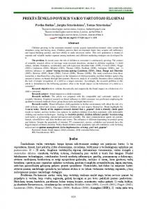
horizontal Field of View (FoV) than the camera that is why we are observing some objects with horizontal features whose vertical counterparts are not detected. Though the camera has smaller horizontal view but its wide vertical sensing range permits it to observe window limits not detected by the laser. Figure 1(b) illustrates the desired representation of the environment with the robot (represented by triangle) and extracted features from both sensors. Laser sensor can display extracted feature immediately but it is almost impossible to display camera extracted feature exactly on the actual location because of unavailability of depth information. These limitations offer several challenges to use both sensors and demand a solution to initialize camera based features immediately and to converge them after getting sufficient parallax [12]. Here we are proposing a unified approach for presenting the features in a common way and to update them in EKF SLAM.
III. PROPOSED APPROACH
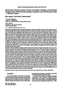
A. Camera Features After image capturing from a calibrated camera, inverse depth parameterization of vertical lines has been incorporated in EKF framework. Consider a robot moving in an indoor environment from point A to point B with initial pose (xA ,yA , θA) to final pose (xB , yB , θB) as shown in Fig. 2. During its motion, it observes a vertical line feature (as shown by solid cyan line), which is projecting on X-Y plane at point V. The bearing of the first vertical line feature is denoted as in the robotic frame of reference as shown by arrow from point A to point V in Fig. 2. The camera frame of reference and robotic frame of reference (shown by XR-YR axis with dashed arrows) are considered as same in this work. A 2D unit vector describing the direction of the line feature from the camera can be represented as (1)
In indoor environments, geometric shapes are common such as tables, walls, chairs and cupboards etc., which need to be modeled. In this work we are detecting these shapes from integrated sensors and extracting lines/corners features from them to model the environment.
a)
l w l xw
T T l yw R wc u0 uc d u / f 0 1 ,
(1)
where is the u-axis (horizontal camera axis) central coordinate in the image, is the focal length of the camera, is the physical spacing of pixel on the optical sensor of the camera, is the rotation matrix from the camera coordinate frame to the world coordinate frame and is the detected u-axis coordinate of the vertical line feature. The bearing can be represented using directional vector as b) Fig. 1. Robot is observing horizontal and vertical lines: (a) environment view; (b) extracted features.
c arctan lxw , l yw .
Figure 1(a) shows the custom-developed robot placed in an indoor environment and getting perception from integrated sensors. These sensors include 2D Hokuyu® laser scanner and a Logitech® webcam based camera. Both of the sensors are positioned at the front center of the robot, with later mounted above the former. From laser scans, horizontal lines (in brown) are extracted which are actually sides of the tables present in the room. The intersections of the sides are also detected as point features (or corners shown with brown circles). From the camera image, vertical lines (in cyan) are extracted which in this case are the end limits of tables and window. Laser sensor has wider
Fig. 2. Vertical lines parameterization.
4
(2)
ELEKTRONIKA IR ELEKTROTECHNIKA, ISSN 1392-1215, VOL. 20, NO. 9, 2014 The world frame is shown by XYZ arrows. The bearing of the feature in world frame ( ) can be computed using
A c .
T
x cos l lxc l cy T Rcw i A RBw . (9) y A sin c
(3) Equation (9) is used to find the horizontal pixel value of the older line for the image feature. Measurement model given by (10) shows the representation for finding the value of predicted older line position ( )
The inverse depth representation for the projected feature point can be given by
fil xA , yA , , i , T
(4)
lc f y 0 u p u0
where ( , ) is the location of the robot in world frame, α is the bearing of the line in world frame and is the inverse of the range (depth) information of the line feature ( ) and is initialized with a guess
i 1/ . Projected coordinates of V (
,
u p u z thu ,
) can be written as
=
lc A l .
flc xA , yA ,lc , dlc , T
.
(13)
where symbolizes laser corner feature, ( , ) is the location of robot at point A, and are bearing (in world frame) and range of the corner from the robot respectively. Corner point coordinates C ( , ) in terms of (13) can be written as
robot at point B in world frame. The older feature location can be predicted using (8) lc
(12)
The corners can be initialized and represented by
, which gives the location of the
T R cw V Aw RBw
(11)
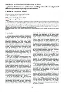
B. Laser Features This work uses laser based horizontal geometrical (line and corner) features and parameterize them as inverse depth features. Consider the same scenario of the robot movement as shown in Fig. 3. At point A, the robot observes a corner C (as pointed by brown arrow) with range (distance from robot) as and bearing as . The laser sensor frame of reference is fixed and is same as the robotic frame of reference. Bearing of the corner feature can be given by (12)
(7)
All the robot poses at A and B are known (with nearest global values) from the motion model. (6) and (7) show that only inverse depth ( ) is unknown and we need to find its value using significant changes of robotic pose as well as feature bearing angles. The proposed approach is based on taking the advantage of the robot successive movement and iteratively predicting a nearer estimate for the point V coordinates. For future matching in upcoming images, an image patch covering all vertical portion of the image with a small width around the line is stored to associate line in future observations. When the robot moves to B and takes an image then the line appears in the image on different horizontal pixel value. To associate this line with the older line, we need to predict a guess for the older line which shows that the older line will probably appear in this horizontal region of the new image shown in pixels. This guess is generated using motion model of the robot. Currently it is assumed that we are getting the pose prediction and
(10)
where is the new observation for current feature and thu is the threshold (in pixels). After getting matched pair, for more robust association, new image patch belonging to a new current feature is compared with previously stored patch through cross correlation. In case at any step, if no line is matching with new line and new line is far from older lines (greater than predefined threshold) then new line is considered as fresh candidate and is initialized immediately.
(6)
During its motion from A to B, the robot is detecting again vertical line with different local bearing in its view as shown by arrow from B to V in Fig. 2. Point coordinates of V take form of (7)
x x cos VBw V B 1/ i . yV yB sin
lxc du
.
To associate new observed lines with the old ones, nearest neighbor method is used. For each new line, it is evaluated that new observation and old prediction satisfy (11)
(5)
x x cos( ) VAw V A 1/ i . yV y A sin( )
x x cos lc C c A dlc . yc y A sin lc
(14)
(8) During motion from A to B, the robot is detecting again corner with different range and bearing (say =
Rewriting (8) in inverse depth form as
5
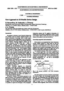
ELEKTRONIKA IR ELEKTROTECHNIKA, ISSN 1392-1215, VOL. 20, NO. 9, 2014 As the robot moves, the line feature will re observe with
) as represented by arrow from B to C in Fig. 3.
different range and bearing (say
=
) as indicated
by arrow from point B in Fig. 4. The prediction ℎ of old line feature is given by
d dll xB cos ll yB sin ll hll hll , ll B hll
where dhll and αhll are the predicted range and bearing for the old line from point B respectively, (xB, yB, θB) is the predicted new robot pose at point B, and are the old line global range and bearing respectively. Each new line feature measurement is tested with old line feature prediction for validating threshold given by
Fig. 3. Laser extracted corner parameterization.
We need to predict old corner feature and to associate this with new observed corner feature. The prediction ℎ of old corner feature is given by
d xc xB 2 yc yB 2 , hlc hlc hlc arctan yc yB , xc xB B
hll zll thll .
(15)
(19)
IV. UNIFIED EKF SLAM Based on fusion of features extracted from both kinds of sensors in the same algorithm, a unified EKF SLAM solution has been proposed.
where dhlc and αhlc are the predicted range and bearing for the old corner from point B respectively, (xB, yB, θB) is the predicted new robot pose at point B and (xC, yC) is the old corner coordinates as determined by (14). In this work, nearest neighbor method is used which is detailed in [17]. Each new corner measurement is tested with (old) prediction against threshold as given by
A. State Vector and Covariance Matrix The state vector X of the EKF SLAM consists of the robot state and features states. All the features are used in the same state vector as shown in (20) T
hlc zlc thlc .
(18)
X xvT , f il T , f lcT , f ll T ,
(16)
(20)
If the re-observed corner is found within a predefined threshold then it firmly associates with the previously seen corner. If no match is found then the corner is treated as new feature and is initialized as given by (13). At the starting location (point A), the robot is observing horizontal lines (in brown) shown in Fig. 4. One such line is pointed by brown arrow from point A in the figure. The detected line is making a global bearing of with range of . Feature initialization is given by
where = , , , , , represents the robot pose and its linear and angular velocities, , and are given by (4), (13) and (17) respectively. The covariance matrix P associated with the state vector X is
fll xA , y A ,ll , dll ,
where represents variances associated with moving robot pose and its velocities, represents variances associated with nth feature (nth feature can be from camera or from laser) and remaining elements show cross co-variances among robot state and feature state.
T
Pxv P P f n xv
(17)
where represents the laser line feature, ( , ) is the location of the robot and and are bearing and range (in world frame) of the observed line respectively. The end points global coordinates for the lines are saved to associate them in future.
Pxv f n , Pf n
(21)
B. Prediction Update In this work, the prediction step of the EKF SLAM uses constant velocities motion model [12]. It is assumed that the linear ( , ) and the angular ( ) accelerations produce impulses of the linear ( × ∆ , × ∆ ) and angular ( × ∆ ) velocities respectively with zero mean and known Gaussian distribution during time period of ∆ which affect the robot state. It gives an update on state vector and covariance matrix which becomes and given by (22) and (23) respectively: T
X xvT , filT , flcT , fllT ,
Fig. 4. Laser extracted line parameterization.
6
(22)
ELEKTRONIKA IR ELEKTROTECHNIKA, ISSN 1392-1215, VOL. 20, NO. 9, 2014
P F P F T G Q GT .
recorded at the starting location with the vertical lines (shown in green) observed from the image. Figure 5(b) indicates the corresponding results of laser lines (in blue) and corner features (in cyan) extracted from the first scan. In this figure, vertical image lines representing inverse-depth projected points (in green with numbering) and current robot location (in red) are also shown. All the vertical lines are just initialized with a predefined value and these positions are not showing the actual locations. Laser scan is covering 210 degrees around the robot, so number of horizontal features is more than extracted vertical line features (which have only 120 degree view).
(23)
The motion prediction only affects the robot state during motion without changing the features state. F and G are represent the Jacobians of motion function , , , w.r.t. system state and w.r.t. noise , , = , , ∆ respectively, Q is represents the covariance matrix for the noise , , as stated in [12]. C. Measurement Update After prediction, in the measurement update step of the algorithm, Kalman gain K is determined by [3]
K P H
H P H T R
1
,
(24)
where is Jacobian of the measurement prediction function w.r.t. the state vector. Three different functions for predicting different sensors as given by (10), (15) and (18) are used in this work. The overall Jacobian is given by (25)
H Hil , Hlc , Hll . T
(a) (b) Fig. 5. First image with lines (a); First scan and lines (axes are in m) (b).
(25)
The robot continues its motion. Figure 6(a) shows final location of the robot (having black square as its identity) while Fig. 6(b) illustrates 2D map with trajectory. The updated laser lines (in blue), laser lines corners (in cyan), vertical image lines showing inverse-depth points (in green) and current robot pose (in red) can be seen in the figure. New vertical lines (in green) are also observed which were not detected at the beginning. Each inverse-depth point, initially initialized with a default value, has now converged to its nearest world location. Successive observations lead to depth estimation and points shift to almost correct locations. Some lines are not converged correctly due to low parallax and problems in data association. Figure 7 presents the resultant partial 3D updated map of the environment and trajectory within it as shown by red marks.
In (24), is the observation noise matrix, which deals with uncertainty of the observations [14]. After determining Kalman gain , state vector and covariance matrix are updated:
X X K z h ,
(26)
P I KH P ,
(27)
where h and z represent the predictions associated with the features and current measurements respectively [12]. This procedure involves final state estimations and its covariance in the current iteration. New features are added after these steps. Though all kinds of features are distinguished w.r.t. different measurements and associated models but a balanced state and covariance updates result in a peaceful and unified solution. V. EXPERIMENTS AND RESULTS An indoor office like environment is selected for experiments having objects with orthogonal and nonorthogonal orientations. The robots are moved manually from different start-end positions to get different trajectories and corresponding laser range data and images have been recorded. The frequency of both sensor inputs is fixed to 10 Hz. Maximum linear speed of each robot is around 0.1 m/sec and maximum angular speed is around 0.03 rad/sec. The different data sets obtained are then used independently in EKF algorithm. The algorithm is developed by combining standard MATLAB functions with various open source functions such as openSLAM developed by research community. Hough transformation function is used to extract image lines while Split and Merge algorithm is used to extract laser lines. In first experiment, the robot is initialized with pose (0, 0, 0). Figure 5(a) illustrates the first image from the camera
(a) (b) Fig. 6. Robot final location (a); final updated map (axis are in m) (b).
Fig. 7. Robot trajectory and partial 3D updated map (axis are in m).
7
ELEKTRONIKA IR ELEKTROTECHNIKA, ISSN 1392-1215, VOL. 20, NO. 9, 2014 In second experiment, another similar robot is also deployed. Assuming that this robot is moving from a known location with a known orientation in the same environment, the first image view from the second robot is shown in Fig. 8(a) with the corresponding laser scan illustrated in Fig. 8(b). In the image, the first robot can also be seen in the view of the second robot (red mark).
compact map model as compared to other representations. It is easy to process and to handle during computation and sharing. Based on experiments, results are found nearly accurate for both kinds of sensors extracted features. For better performance of the proposed method, it is noticed that for image features, extraction and association of more features are required. The developed map model finds its potential in various applications requiring real-time survey of environment, 3D modeling, building map for robot navigation and path planning. Results can also beneficiate human assistance to accomplish various tasks. REFERENCES [1]
[2]
(a) (b) Fig. 8. Second robot first view from camera (a); first laser scan (axes are in m) (b).
[3] [4] [5]
[6]
[7]
[8] Fig. 9. Partial 3D Global map and robots trajectories (axes are in m). [9]
Second robot continues its motion and keeps building its map. Due to known location of the second robot w.r.t. the first one, the second robot poses and its map can be plotted in the same map model of the first robot (shown in Fig. 7). Figure 9 shows trajectories of the first and second robot in red and blue respectively in the resultant partial 3D global map of the environment. It is important to note that vertical and horizontal lines are increased as second robot has explored environment with different views as compared to first robot exploration. Table I shows the mean features position error when compared with their actual locations in the environment with the developed map model.
[10]
[11]
[12] [13]
[14]
TABLE I. FEATURES MEAN POSITION ERRORS. Robot no. Laser feature error (in cm) Image feature error (in cm) 1 15 27 2 17 35
[15]
[16]
VI. CONCLUSIONS A unified EKF SLAM framework is proposed and tested in an indoor environment for building partial 3D map by using more than one robot. The proposed method provides a
[17]
8
H. D. White, T. Bailey, “Simultaneous localization and mapping: part 1”, IEEE Robot. Automat. Mag., vol. 13, no. 2, pp. 99–110, 2006. [Online]. Available: http://dx.doi.org/10.1109/MRA.2006.1638022 J. Aulinas, Y. Petillot, J. Salvi, X. Llado, “The SLAM problem: a survey”, in Proc. Conf. on Artificial Intelligence Research and Development, Spain, 2008, pp. 363–371. S. Thrun, W. Burgard, D. Fox, Probabilistic Robotics. MIT Press 2005. B. Siciliano, O. Khatib, Hand Book of Robotics, Springer. 2008. [Online]. Available: http://dx.doi.org/10.1007/978-3-540-30301-5 A. Garulli, A. Giannitrapani, A. Rossi, A. Vicino, “Mobile robot SLAM for line-based environment representation”, in Proc. 44th IEEE Conf. on Decision and Control, Spain, 2005, pp. 2041–2046. [Online]. Available: http://dx.doi.org/10.1109/CDC.2005.1582461 S. Thrun, Y. Liu, D. Koller, A. Ng, Z. Ghahramani, D. Whyte, “Simultaneous localization and mapping with sparse extended information filters”, Int. J. Robot. Res., vol. 23, no. 7, pp. 693–716, 2004. [Online]. Available: http://dx.doi.org/10.1177/ 0278364904045479 S. Riaz, L. Braydaand, R. Chellali, “Distributed feature based multi robot SLAM”, in Proc. IEEE Int. Conf. on Robotics and Biomimetics, Thailand, 2011, pp. 1066–1071. D. Hahnel , W. Burgard , D. Fox, S. Thrun, “An efficient fast-SLAM algorithm for generating maps of large-scale cyclic environments from raw laser range measurements”, in Proc. IEEE/RSJ Int. Conf. Intelligent Robots Systems, Las Vegas, USA, 2003, pp. 206–211. J. Sola, T. Calleja, J. Civera, J. Montiel, “Impact of landmark parameterization on monocular EKF SLAM with points and lines”, Int. J. Comput. Vis., vol. 97, no. 3, pp. 339–368, 2012. [Online]. Available: http://dx.doi.org/10.1007/s11263-011-0492-5 N. Muhammad, D. Fofi, S. Ainouz, “Current state of the art of vision based SLAM”, in Proc. Int. Society for Optics and Photonics Technology (SPIE) Conf., California, USA, 2009, pp. 12. T. Lemaire, S. Lacroix, J. Sola, “A practical 3D bearing only SLAM algorithm”, in Proc. IEEE/RSJ Int. Conf. Intelligent Robots Systems, Canada, 2005, pp. 2449–2454. J. Civera, A. Davison, J. Montiel, Structure from motion using the extended Kalman filter, Springer tracts in Advanced Robotics, 2012. J. Montiel, J. Civera, A. Davison, “Unified inverse depth parameterization for monocular SLAM”, in Proc. Robotics, Science and Systems, Pennsylvania, USA, 2006, pp. 16–19. A. P. Gee, W. Mayol, “Real-time model-based SLAM using line segments”, in Proc. 2nd Int. Symp. Visual Computing, Nevada, USA, 2006, pp. 354–363. P. Smith, I. Reid, A. Davison, “Real-time monocular SLAM with straight lines”, in Proc. British Machine Vision Conf., Edinburgh, UK, 2006, pp 17–26. A. Davison, I. Reid, N. Molton, O. Stasse, “MonoSLAM: Real-time single camera SLAM”, IEEE Trans. Pattern Anal. Mach. Intell., vol. 29, no. 6, pp. 1052–1067, 2007. [Online]. Available: http://dx.doi.org/ 10.1109/TPAMI.2007.1049 S. Riaz, Z. Li, A. Ahmed, R. Chellali, “Laser only feature based multi robot SLAM”, in Proc. IEEE Int. Conf. on Control, Automation, Robotics and Vision, China, 2012, pp. 1012–1017.