A Uniform Clustering Mechanism for Wireless Sensor Networks

Hindawi Publishing Corporation International Journal of Distributed Sensor Networks Volume 2014, Article ID 924012, 14 pages http://dx.doi.org/10.1155/2014/924012

Research Article A Uniform Clustering Mechanism for Wireless Sensor Networks Rabia Noor Enam,1 Rehan Qureshi,2 and Syed Misbahuddin1 1 2

Department of Computer Engineering, Sir Syed University of Engineering and Technology, Karachi 75300, Pakistan Department of Telecommunication Engineering, Sir Syed University of Engineering and Technology, Karachi 75300, Pakistan

Correspondence should be addressed to Rabia Noor Enam; afaq [email protected] Received 25 July 2013; Revised 22 January 2014; Accepted 10 February 2014; Published 23 March 2014 Academic Editor: KingShan Lui Copyright © 2014 Rabia Noor Enam et al. This is an open access article distributed under the Creative Commons Attribution License, which permits unrestricted use, distribution, and reproduction in any medium, provided the original work is properly cited. In wireless sensor networks with dynamic clustering, the cluster heads are usually not selected on the basis of their locations. This causes irregular distribution of cluster heads and highly variable number of nodes in the clusters. Also, some of the clusters are spread over large areas within the network, causing limited spatial correlation between associated sensor nodes. These irregularities in cluster placements and dimensions negatively impact the efficiency of a wireless sensor network. For example, for a cooperative data aggregation, it necessitates variable or large sized packets while the aggregations, based on spatial correlation of sensor nodes, cannot be exploited easily. In this paper, we have developed a Distributed Uniform Clustering Algorithm (DUCA) for cluster based WSN. In DUCA, cluster formation mechanism is based on a virtual-grid system and sensing ranges of nodes that provide even distribution of clusters, homogenized cluster sizes, and reduced energy consumption. Simulation results show that DUCA improves the distribution of cluster heads by more than 2 times and reduces the energy consumption within a range of 15% to 50% as compared to the existing protocols.

1. Introduction The basic job of a wireless sensor network (WSN) is to sense and collect the physical or quantifiable data from its surroundings and forward it to some central location. The central location may possibly be an isolated system or it could be a part of a globally stretched infrastructure, for example, the Internet of Things (IoT). The IoT, as envisioned, consists of data sensing and collecting objects, attached to communication devices, providing data that can be analysed and used to initiate automated actions. It has been estimated that by 2015 there will be around 25 billion devices wirelessly connected around the globe [1]. This has created a new perception of incorporating WSN as data collecting component of IoT. However, this requires much larger and wide-ranging sensor networks than currently being imagined [2]. Cooperative energy efficient data collection from such network puts new challenges on the system. In a large scale WSN, usually, the nodes collaborate with each other to collect and forward data in a hierarchal manner. For this purpose, cluster based protocols are commonly employed. In majority of the cluster based protocols, the clusters

are formed dynamically and repeatedly to collect the data from multiple sensor nodes. Usually the dynamic cluster based protocols have highly variable-sized clusters which are not formed uniformly, for example, in LEACH [3], HEED [4], EAP [5], and TDEEC [6]. By “cluster size” we mean the number of nodes in a cluster. Due to the irregular placement of sensor nodes and variable sizes of clusters, we need to have variable or large sized packets for data collection and aggregation. On the contrary, it has been shown in the previous research works that due to the limitations and resource constraints of a WSN, its optimal packet size should be small and should have fixed length [7, 8]. These packet sizes can be constrained by homogenizing cluster sizes in a WSN. In this work our main objective is to develop a uniform cluster formation mechanism for WSNs without consuming extra energy of the network. For this purpose, we have proposed a new solution which can develop homogeneous clusters in terms of number of nodes with reduced variations in the cluster sizes. In our proposed mechanism the even distribution of cluster heads and clusters is achieved by implementing an energy efficient usage of virtual grids in the network. Unlike previously proposed grid-cluster based protocols, in

2

International Journal of Distributed Sensor Networks

Cluster 4

Cluster 1

Cluster 5 Sink

Sink Cluster 3

Cluster heads Cluster 2

Cluster 7

Cluster 8 (a) Cluster heads selected in a round

Cluster 6

(b) Formation of irregular sized clusters

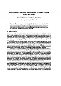
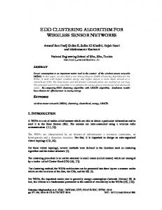
Figure 1: Dynamic cluster based WSN.

our mechanism a grid is not taken as a cluster rather clusters are formed on the basis of distances of nodes to their nearest cluster heads. The sizes of clusters are further reduced by exploiting the redundant and overlapped sensing ranges, which occur due to the random placements of sensor nodes in the network. The remaining paper is organized as follows. Section 2 further explains the problems that arise due to the highly variable sized clusters in WSNs. Section 3 gives a brief overview of the methods given in current literature to solve the problem. Section 4 explains the proposed algorithm design and compares it with the existing protocols. Section 5 discusses a heuristic approach that can be used to reduce the cluster sizes by exploiting the sensing ranges of the nodes. In Section 6, a mathematical relationship is presented that finds the optimum number of grids in the network for a given number of sensor nodes. Section 7 evaluates our proposal against centrally controlled based and grid-cluster based protocols using simulations. Finally, Section 8 concludes the paper.

2. Variable Sized Clusters in a Dynamic Cluster Based WSN In many of the dynamic cluster based protocols like [3–6, 9– 11], the location of the CHs is not considered in the CHselection criteria. As a result, the selected CHs are not uniformly distributed in the region. For example, it can be seen in Figure 1(a) that all of the CHs are formed in the lower right corner of the network area (Figure 1(a) is a snap shot of one of the rounds taken from a simulation of LEACH protocol [3]). This type of nonuniform selection of CHs has created the following side effects on the system. (1) The sizes of clusters, in terms of number of nodes per cluster, are highly variable as shown in Figure 1(b). This results in the requirement of large or variable sized packets for the aggregation of data. On the other

hand, due to resource constraints, the optimal packet sizes in WSNs are considered to be small and of fixed length [7, 8, 12]. (2) There are some clusters in the network which are spread on large regions. This implies that there must be several nodes which have to contact distantly located CHs to forward their data, for example, clusters 1 and 2 in Figure 1(b). Also, the data at the CHs of these clusters must be collected from far off areas of the region. This influences the system in two ways. (a) The distant nodes in large sized clusters need to spend higher energy to transmit the data to their CHs. According to the free space energy consumption relation (see (1)), energy consumed in the transmission of 𝑘 bit (𝐸𝑇𝑋 ) is dependent majorly on two factors: size of the data packet (𝑘) and the distance between the source and destination (𝑑). 𝐸elec and 𝐸amp are the energies consumed in electronic circuitry and the amplification power of the node, respectively. These energies are kept constant for a given node type: 𝐸𝑇𝑋 (𝑘, 𝑑) = 𝐸elec × 𝑘 + 𝐸amp × 𝑘 × 𝑑2 .

(1)

(b) Usually in WSNs the sensor nodes placed in close vicinity have spatial correlation. Therefore, CHs after collecting data from these nodes aggregate the data into a single packet. These aggregations are usually based on simple rules of taking average, sum, difference, or maximum of the correlated data. These methods of aggregations are also called “summary based” aggregation. In large sized clusters with sensor nodes placed at far off distances, there is less chance of having good degree of spatial correlation among the data. Therefore, logical and balanced aggregation of data cannot be used easily.


3

3. Related Work Some solutions have been proposed in the past to overcome the variations in the cluster sizes of WSN. We have divided these mechanisms into two categories: (1) centrally controlled cluster formation protocols; (2) grid-cluster based protocols.

2

1

5

3

6

Drawback. In centrally controlled cluster formation protocols in order to provide the energy and location status of nodes, all nodes should send extra overhead of control packets at the start of each round [3]. Besides, each node needs to remain in idle listening mode for a considerable time, in order to receive its CH IDs and TDMA schedules. Whether it is a single hop or a multihop network, additional communication cost is incurred. This cost further increases with the size of network or if nodes are placed at far off places in the network.

9

13

10

14

8

7 Sink

3.1. Centrally Controlled Cluster Formation Protocols. In these protocols the clusters are formed dynamically but the process is controlled centrally by the sink. For example, in Base Station Controlled Dynamic Clustering Protocol (BCDCP) [13], at the start of each round, all nodes send their current energy status to the sink. The sink chooses a set of CH candidates based on their energy levels. To get a set of clusters with approximately equal sizes, the sink runs the cluster splitting algorithm iteratively. In each iteration step the algorithm selects the CHs by maximizing the distances between the selected CHs, therefore creating uniformly placed CHs in the network. To form clusters, the nodes are associated to the CHs based on the closest distance. Once the clusters are formed, the extra nodes are handed and taken over between the two neighbour clusters in order to balance the size of the clusters. This whole process is centrally controlled by the sink node. In LEACH-C [3] at the start of each cluster formation round, each node sends its residual energy level and location information to the sink node. The sink node selects CHs and builds clusters using the simulated annealing algorithm. Once the CHs and associated nodes are determined, the sink broadcasts CH IDs and Time Division Multiple Access (TDMA) schedules for each node. All nodes look for their IDs to be matched as the CH ID, if not matched then the nodes follow the Time Division Multiple Access (TDMA) schedule to broadcast their data. The data transmission phase of LEACHC is identical to that of LEACH. This way the sink, knowing the global information of nodes, forms more uniform sized clusters. Similar procedure has been adapted in Cluster-Based Energy-Efficient Data Collecting and Aggregation Protocol (CEDCAP) [14]. After receiving the knowledge of energy levels and locations of all nodes, the sink selects the CHs and their associated nodes. Like LEACH-C, here also sink provides the data transmission TDMA schedules to all nodes. But in CEDCAP, the TDMA calculated by the sink are scheduled according to the node degree control of each cluster. Based on the node degree control a set of nodes in each cluster are kept dormant for some period of time, hence reducing the redundant data transmission in the network.

4

Cluster heads

11

15

12

16

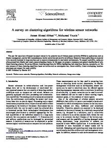
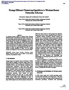
Figure 2: Grid-cluster based WSN.

3.2. Grid-Cluster Based Protocols. Unlike centrally controlled cluster formation protocols, in grid-cluster based protocols the CH selection decisions are distributed among the nodes themselves. Therefore, it can work well in a large scale network. The basic idea of grid-cluster protocols is to divide the network area into equal sized virtual grids where each grid is considered as a cluster with one CH in each cluster [15–20]. The role of CH is rotated among different nodes within a cluster. Figure 2 depicts the grid-cluster method where every grid contains one CH. The main characteristics of the gridcluster based protocols can be given as follows. (1) A grid is considered as a cluster; that is, the clusters are fixed and not dynamic. Although this method decreases the variations in sizes and locations of the clusters, due to the random deployment of nodes, it cannot create all equal sized clusters. Authors in [18] have tried to further even out this irregularity such that after setting one CH in each grid, the sizes of clusters are adjusted by handing and taking over extra nodes to and from the neighbour grids. This is done through a centralized control system and requires an extra overhead of control packets which consumes extra energy and delay in the system. (2) Each grid contains one CH in it and the role of CH rotates among the nodes within a grid. For example, in [16, 20], there is a rotation of CHs which is based on a back-off timer. The back-off timer is calculated on the basis of residual energy levels of each node within a grid. In some of the grid-cluster protocols, the algorithm selects one CH per grid based on its energy level, while there is no rotation of CHs made until the energy of existing CH is completely depleted [17, 19]. Drawback. Grid-cluster protocols have regularized the CH distributions, in the network, to some extent and have substantially reduced the variations in the cluster sizes. But the

4


network energy consumed in these protocols is very high compared to a dynamic cluster based protocol. The reason behind this is that the selection of CHs is done only within a grid and not with respect to the whole network, as is done in LEACH. Therefore, this method does not give a fair selection of CH with respect to all of the nodes of the network. Another reason of high energy consumption is that the clusters are not formed on the basis of the distances to the closest CHs. Irrespective of the distance a node will always have to associate with the CH belonging to its own grid. For example, in Figure 2 in grid number 1 the nodes in the lower right corner of the grid will have to transmit their data to the distant CH in their grid, whereas there were two closer CHs available in grid number 2 and 5.

4.2.1. Detection of Grid IDs. Suppose the network is spread on a rectangular or square area with the dimensions of 𝑋 by 𝑌 units (for the sake of simplicity, in our simulations we have assumed a square area). The sink calculates and assigns grid IDs to all sensor nodes in the network, based on the following steps.

4. Proposed Solution

Steps

In this research work we have proposed a Distributed Uniform Clustering Algorithm (DUCA) to distribute the CHs evenly and to reduce the variations in cluster sizes in a dynamic cluster based WSN. In DUCA to get an even distribution of CHs, the network is divided into virtual grids. Unlike existing grid-cluster based protocols, the grids in DUCA do not represent a cluster. Our suggested CH selection and node association mechanism has substantially reduced the network energy consumptions compared to existing grid-cluster protocols and LEACH-C as a centrally controlled protocol. 4.1. Assumptions. Following are the basic assumptions made in DUCA design. (i) Initially a large number of equally charged sensor nodes are randomly deployed in the field and there is a sink node in the centre of the field. (ii) Each sensor node is stationary after deployment and is capable of getting its location information by the use of global positioning system or by using any other method of localization. (iii) Initially based on their locations each node is informed about their respective grid ID. (iv) Design of the DUCA is such that it does not require any change in the existing MAC layer of a dynamic cluster based protocol. All the contentions in DUCA are solved by the MAC layer proposed for LEACH protocol. 4.2. Algorithm Design. In DUCA, initially the sink decides the required number of CHs (𝐶) in the network. To distribute the CHs evenly, network area is divided into 𝐺𝑇 number of grids such that we get 𝐶 ≈ 𝐺𝑇 . DUCA requires that each sensor node should know which grid it belongs to. In Section 4.2.1, we have explained the method and algorithm used to calculate the grid IDs for each node. In DUCA, like other existing cluster based protocols, the collection of data is done in rounds, whereas the cluster formation process is divided into three phases. CH selections are done in the first two phases (explained in Sections 4.2.2 and

4.2.3, resp.) and node associations are done in the third phase (explained in Section 4.2.4). To make sure that we get at least one CH in almost every grid, more than required number of CHs are preelected in the first phase of CH election. This is done so that after going through the second phase of CH election we can get the required number of evenly distributed CHs in the field.

(1) Sink divides the network area into equal sized 𝐺𝑇 number of virtual grids. Each grid is assigned its ID according to its row number and column number in the field, calculated as follows. Let 𝐺 = grids in one column = grids in one row. The height and width of each grid are 𝐺height = 𝑌/√𝐺𝑇 and 𝐺width = 𝑋/√𝐺𝑇 , respectively. Based on the row number and column number of each grid, their grid IDs are calculated using the following, where 𝑖 is the grid ID of 𝑖th grid: 𝐺𝑖Row

𝑖 𝑖 { for (( ) − ⌊ ⌋) = 0 {𝐺 𝐺 𝐺 ={ {{(( 𝑖 ) − ⌊ 𝑖 ⌋) × 𝐺} elsewhere { 𝐺 𝐺 𝑖 Grid𝑖Col = ⌈( )⌉ . 𝐺

(2)

And midpoint of 𝑖th grid can be calculated as follows: 1 𝐺𝑖Mid = (𝐺height × (𝐺𝑖Col − )) 2

1 by (𝐺width ×(𝐺𝑖Row − )) . 2 (3)

(2) Each node sends its location information (𝑥, 𝑦 coordinates) to the sink. The sink uses Algorithm 1 to calculate the grid ID for each node. (3) Sink broadcasts the grid IDs of all nodes so that every node, for the rest of its lifetime, knows its location and to which grid it belongs to. Table 1 shows all the symbols and their meanings used in this paper. 4.2.2. CH Election Phase 1. In this phase our aim is to get a fair selection of CHs to equalize the consumption of energy among all the nodes in the network. Therefore, the CHs are elected based on the number of times they have been selected in the previous rounds. For this the election method has been adopted from the LEACH protocol. According to LEACH, in every round, each node generates a random number between


5

for 𝑗 = 𝐹𝑖𝑟𝑠𝑡𝑁𝑜𝑑𝑒 to 𝐿𝑎𝑠𝑡𝑛𝑜𝑑𝑒 do Initialize: Grid𝑖 = 1 for 𝑔𝑥 = 1 to 𝐺 do if 𝑥 coordinate of 𝑗 ≤ (𝐺width × 𝑔𝑥) then for 𝑔𝑦 = 1 to 𝐺 do if 𝑦 coordinate of 𝑗 ≤ (𝐺height × 𝑔𝑦) then Assign GridID of 𝑗 = Grid𝑖 break end if Increment: Grid𝑖 by 1 end for break end if Increment: Grid𝑖 = (𝑔𝑥 × 𝐺) + 1 end for end for Algorithm 1: Algorithm to assign Grid-IDs to each node based on their locations.

Table 1: Symbols and their definitions. Symbols 𝑛 𝐶 𝐺𝑇 TR𝑠 𝑅𝑠 𝑅max 𝑆 𝑟𝑠 𝐺height 𝐺width 𝐺𝑖Row 𝐺𝑖Col 𝐺𝑖Mid 𝐺 𝐺CH 𝐺CHmax 𝑑

Definitions Number of nodes in the network Number of Cluster heads Total Number of Grids Threshold Sensing Range Sensing range of a sensor node Maximum required sensing range Side Length of the network area Height of each grid Width of each grid Row number of 𝑖th grid Column number of 𝑖th grid Mid Point of 𝑖th grid Grids in one row or column Number of grids that have the highest probability of having one CH in each grid Maximum number of grids beyond which the probability of having one CH in each grid starts decreasing Percentage of distortion in data after its aggregation

0 and 1 and if the number is less than a threshold value 𝑇(𝑛), the node gets elected for that round. The value of 𝑇(𝑛) is calculated as follows [3]: 𝑝CH { 𝑇 (𝑛) = { 1 − 𝑝CH ∗ (𝑟 mod (1/𝑝CH )) {0

for 𝑛 ∈ 𝑋

(4)

otherwise.

𝑝CH is the required percentage of CH in the network; that is, 𝑝CH = 𝐶/𝑛, where 𝑛 is the total number of nodes in the network and 𝑋 is the set of nodes that have not been cluster heads

in the last 1/𝑝CH rounds. 𝑟 is the round number for which the CH is being elected. If taken average over a large number of rounds, LEACH’s 𝑇(𝑛) formula always gives exact value of 𝑝CH , while in an individual round it highly deviates from the required value of 𝑝CH . Thus, by using LEACH’s 𝑇(𝑛) formula in DUCA’s first phase of CH selection, it was found that there are many rounds, where 𝐶 ≪ 𝐺𝑇 . As a result, the relation 𝐶 ≈ 𝐺𝑇 could not be achieved in DUCA’s second phase of CH selection. In DUCA more number of CHs are needed to be preelected than eventually required; that is, we need to keep 𝑝CH > 𝐶/𝑛. But increasing the value of 𝑝CH gives a corresponding increase of network energy consumption. The reason behind this increase of energy consumption is that with a larger value of 𝑝CH the CHs are not elected fairly based on their previous number of selections. Question arises: how much greater should we keep the value of 𝑝CH so that the number of nodes elected in this phase is large enough to get at least one CH in each grid but not large so that it would consume a considerable amount of extra energy. We have estimated the value of 𝑝CH as follows. Let 𝑃 be the probability that almost every grid contains at least one CH after first phase of CH election; then, we have to maximize 𝑃 such that 𝐺𝑇 ≤ 𝑝CH < 𝑛, 𝑛

𝐸𝑐 < 𝐸𝑐𝐺,

(5)

where 𝐸𝑐 is the network energy consumed in our algorithm for 𝐶 number of cluster heads and 𝐸𝑐𝐺 is the network energy consumed in a grid-cluster based algorithm for 𝐶 number of cluster heads. It was seen through the results based on extensive simulations of the proposed method that if 𝑝 is increased by 𝐺𝑇 times in (4), then optimal number of preelected CHs can be obtained with minimal extra energy consumptions. 4.2.3. CH Election Phase 2. The preelected CHs in phase 1 are not evenly distributed; therefore, the aim of this phase is to

6


Require: Put all nodes in the ASST LIST into IDLE STATE Initialize: ACTIVE LIST ← ASST LIST From ASST LIST for 𝑖 = 𝐹𝑖𝑟𝑠𝑡𝑁𝑜𝑑𝑒 to 𝑆𝑒𝑐𝑜𝑛𝑑𝐿𝑎𝑠𝑡𝑛𝑜𝑑𝑒 do for 𝑗 = 𝑁𝑒𝑥𝑡𝑁𝑜𝑑𝑒 to 𝐿𝑎𝑠𝑡𝑁𝑜𝑑𝑒 do if The distance between 𝑖 & 𝑗 ≤ TR𝑠 then if 𝑖 ∈ ACTIVE STATE then Put 𝑗 ∈ SLEEP STATE else if 𝐸𝑖 ≥ 𝐸𝑗 then Put 𝑖 ∈ ACTIVE STATE and 𝑗 ∈ SLEEP STATE Decrease 𝑗 from the ACTIVE LIST else Put 𝑗 ∈ ACTIVE STATE and 𝑖 ∈ SLEEP STATE Decrease 𝑖 from the ACTIVE LIST end if end if end for end for Ensure: TDMA Schedule ← ACTIVE LIST Algorithm 2: Algorithm to select associate nodes based on TR𝑠 .

get an even distribution of CHs in the network. Following are the steps taken.

aggregate, and forward data to the sink. The clusters are formed based on the following steps.

Steps

Steps

(1) All the CHs elected in phase 1 broadcast their residual energy levels and their grid IDs within their grid region. (2) If there were more than one CH in a grid, after hearing the broadcast in Step 1, the one with the highest energy level gets itself elected automatically. The remaining CHs, belonging to the same grid, will go back into their normal node mode for this round. (3) The elected CHs, finally, advertise their elections. This time, the broadcast range is increased to cover the nodes in the adjacent grids also. This is done because DUCA tries to get 𝐶 ≈ 𝐺𝑇 and not 𝐶 = 𝐺𝑇 . It means that there is a small possibility in few rounds that there exists a grid which has no CH in it. In that case the nodes in the grid without a CH can associate themselves with the closest CH in adjacent grid. This method gives number of CHs elected as almost equals to the number of grids in the region; that is, 𝐶 ≈ 𝐺𝑇 , and if the ratio of 𝑛/𝐺𝑇 is according to (11) (explained in Section 6) we get the number of CHs exactly equal to the number of grids; that is, 𝐶 = 𝐺𝑇 . 4.2.4. Nodes Association Phase. The remaining nodes, after hearing CH advertisements, determine their closest CH on the basis of received signal strengths of multiple CHs. In this phase we have used a parameter, namely, Threshold Sensing Range (TR𝑠 ), to further reduce the sizes of clusters. It is assumed that the acceptable value of TR𝑠 which is based on the sensing range of nodes is provided by the sink (in Section 5 we have explained a method to suggest a suitable value for TR𝑠 ). Once all the clusters are set, CHs collect,

(1) Irrespective of their grid IDs, nodes broadcast their association requests to the CH, which has the shortest distance to them. In these broadcasts, the nodes also send their residual energy levels and their locations to the respective CHs. (2) CHs calculate the distances between each of its associated nodes and select the active nodes for this round according to the algorithm shown in Algorithm 2. ASST LIST is the list of nodes which are associated to this CH and the ACTIVE LIST is the list of nodes which are active for this round only. (3) The CH puts a node to either SLEEP STATE or ACTIVE STATE depending on TR𝑠 value between the nodes and the energy level 𝐸𝑁 of the node 𝑁. The CHs provide slots in the TDMA schedules only for the ACTIVE STATE nodes and the redundant nodes remain in SLEEP STATE for this round. 4.3. Comparisons of Proposed Algorithm with Centrally Controlled and Grid-Cluster Based Protocols. The comparison analysis of DUCA with the centrally controlled and gridcluster based protocols are given as follows. (1) The startup phase in centrally controlled cluster formation protocol is always more energy intensive than the distributed approach since the information from each node must be transmitted to the sink at the beginning of each round [3]. This cost of communication increases for the nodes that are far away from the sink [3]. This is not the case with our algorithm since it is based on distributed clustering method.

International Journal of Distributed Sensor Networks (2) Unlike centrally controlled protocol the CH selection decision is distributed among the nodes; therefore, the proposed algorithm can be used in a large scale network with reduced overheads. (3) Unlike existing grid-cluster based protocols, the grids used in our algorithm is only for the even distribution of CHs and not for the cluster formations. Our suggested CH selection and node association mechanism have substantially reduced the overall energy consumption of the network compared to the existing grid-cluster based protocol. There are following main points that can differentiate our mechanism with any other grid-cluster based protocol proposed so far. (a) With randomly deployed nodes there can be many grids which have small number of nodes. Therefore, using CH selections criteria only within the grids could not give fair CH selections based on overall number of nodes in the network. This can be explained as follows. For example, in Figure 2, grid numbers 8 and 5 have only three nodes in each of them. If these three nodes become CH alternatively, the chances of their expiring as compared to other nodes in the network will be very high. Therefore, a simple rule of selecting one CH per grid as considered in existing grid-cluster based protocols does not give a balanced consumption of the network energy. That is why in DUCA, every grid does not necessarily contain one CH in it. However, we try to maintain the relation as 𝐶 ≈ 𝐺𝑇 . (b) In DUCA, a grid does not necessarily represent a cluster; rather, a cluster is formed based on the distances of each node to its nearest CH. As a result, a CH may have its associated nodes from more than one grid while maintaining even distribution of clusters and lower energy expenditure in the network. (c) In our algorithm based on a parameter, introduced as Threshold Sensing Range TR𝑠 < 𝑅𝑠 , the sizes of clusters are further reduced by selecting only those nodes which do not fall within TR𝑠 range of each other. (d) Unlike existing grid-cluster based protocol, in DUCA not all of the grids must be containing one CH for the entire time period. There may be few grids which would remain without CHs in some of the rounds. The overall effect after the implementation of the DUCA is that we are now able to have the following: (1) cluster heads and clusters, as evenly spread in the network; (2) a significant improvement in the energy consumption as compared to a regular grid-cluster based protocol; (3) the selection of CHs is done locally and there is no need of centralized CH selections by the sink;

7 (4) in each grid only those nodes will be elected as CHs which have the highest residual energies; (5) the sizes of clusters are in a limited range and the clusters are confined in a close vicinity. This helps in appropriate aggregation of the data specially within a small sized data packet.

5. A Heuristic Approach to Determine the Threshold Sensing Range (TRs ) In our algorithm using a suitable value of Threshold Sensing Range (TR𝑠 ) can reduce the sizes of clusters and the redundant data flow in the network. In this section we will discuss a method through which the value of TR𝑠 can be estimated in a network of randomly deployed sensor nodes. A network is said to be covered if each point of it is covered by the sensing range of at least one node. In a randomly deployed WSN, to guarantee the coverage of the whole area, generally more sensors are deployed than needed. This is done so that the sensing or monitoring tasks can be performed to compensate the lack of exact positioning and to improve the fault tolerance [21]. On the other hand, this creates many regions in the network which are covered by more than one sensing node. These regions cause redundant flow of data packets in the network, thus creating unnecessary energy consumption of the network. In DUCA, the parameter TR𝑠 < 𝑅𝑠 has been used by the CHs to further reduce their cluster sizes, by selecting only those nodes which do not fall within the TR𝑠 range of each other (Algorithm 2). In a large scale randomly deployed network of sensor nodes, there are three ways through which an acceptable value of TR𝑠 can be estimated: (1) application requirement; (2) deployment strategy of the nodes; (3) the number of nodes deployed in the area. Based on the application requirements, approximating the value of TR𝑠 is beyond the scope of this paper discussion. However, based on the deployment strategy and the number of nodes in the network, an approximate value of TR𝑠 can be estimated as follows. 5.1. Calculation of TRs . Let 𝑛 be the minimal number of nodes, required for an optimal and deterministic (not random) placement of nodes (i.e., each point of the network area is covered with at least one sensor node). Then, the relation between 𝑛 and the sensing ranges 𝑅𝑠 of nodes can be given as follows [22]: 𝑛 × 𝜋𝑅𝑠2 2𝜋 , = √27 𝐴

(6)

where 𝐴 is the size of the monitored area and 𝑅𝑠 is assumed to be same for all the nodes. When nodes are deployed randomly, their placements are assumed to be uniformly distributed. It means that each node has equal probability to be placed at any location within the

8


(a) Best case

rs

Rs

rs

Rs

(b) Worst case

Figure 3: The best and worst case scenarios for randomly deployed nodes in a square region.

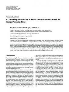
area. It can intuitively be said that to have a minimum value of 𝑅𝑠 the nodes should be placed evenly and equidistantly. This can be called the best case, whereas worst case would be when all of the nodes have fallen at one location which is the farthest point to the center of the field. A square region in Figure 3, with its sides as 𝑟𝑠 and area size as 𝐴 = 𝑟𝑠2 , explains the best and worst placements of nodes based on the minimum requirement of 𝑅𝑠 . From (6), we can say that with 𝑛 evenly placed nodes, to have the whole area covered, the sensing range required for each node can be given as

Rmax s

Rs

l TRs Rs Sensing nodes

𝑅𝑠 = √ 0.38 ×

𝑟𝑠2 𝑛

𝑟 or 𝑅𝑠 = 0.62 × 𝑠 . √𝑛

(7) Figure 4: Threshold Sensing Range (TR𝑠 ) between two nodes.

From Figure 3, for the worst case is the longest distance between the two points of a square region; that is, a diagonal of a square, given as 𝑅𝑠 = √2 × 𝑟𝑠 . In the process of random deployment of nodes, if 𝑝 is the probability that the nodes are arranged according to the best case then (1−𝑝) is the probability that the nodes are deployed as worst case. Therefore, the minimum sensing range 𝑅𝑠 that each node should have can be given as 𝑅𝑠 = (0.62 ×

𝑟𝑠 ) (𝑝) + √2 × 𝑟𝑠 (1 − 𝑝) . √𝑛

(8)

TR𝑠 is the distance between two nodes in a network which are sensing almost the same region of the network, shown in Figure 4, and can be given as TR𝑠 = 2 × (𝑙 − (𝑅𝑠 − 𝑅max 𝑠 )) ,

(9)

where 𝑅𝑠 is the available sensing range, 𝑅max 𝑠 is the maximum required sensing range, and 𝑙 is the difference between outer boundaries of 𝑅𝑠 and 𝑅max 𝑠 . From (8) and (9), for 𝑅𝑠 > 𝑅max 𝑠

and considering worst and best case scenarios in a randomly deployed network, the value of TR𝑠 can be estimated as TR𝑠 = 2 × (𝑙 − ((0.62 ×

𝑟𝑠 ) (𝑝) √𝑛

(10)

+√2 × 𝑟𝑠 (1 − 𝑝) − 𝑅max 𝑠 )) . Table 1 shows all the symbols and their meanings used in this paper.

6. Relation between Number of Nodes, Grids, and Cluster Heads in the Network In DUCA, to get the desired number of CHs, the network is divided into the same number of virtual grids. In this section we will explore the relation between 𝐺𝑇 , 𝑛, and 𝐶 in a network of randomly deployed nodes. It was seen during the implementation of our proposed algorithm that for a small value of 𝐺𝑇 the relation 𝐶 ≈ 𝐺𝑇 can

GCHmax

International Journal of Distributed Sensor Networks 90 80 70 60 50 40 30 20 10 0

9 (3) LEACH-C protocol: as an example of centrally controlled uniform cluster formation protocol.

y = 0.241x + 6.451

Our aim is to show that our proposed mechanism gives a better solution, in terms of cluster sizes and distributions, compared to LEACH protocol while giving a substantial decrease of network energy consumption compared to gridcluster and LEACH-C protocols.

0

50

100 150 200 250 Total number of nodes (n)

300

350

Figure 5: Upper limit of 𝐺CH for different value of 𝑛.

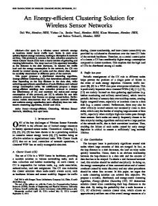
easily be maintained; that is, almost every grid contains one CH in it, whereas this relation cannot be achieved for lower values of 𝑛 or higher values of 𝐺𝑇 . Through an extensive simulation of our proposed algorithm, we have developed a formula to find the minimum value of 𝑛 that can be suggested prior to the network deployment such that the relationship of 𝐶 ≈ 𝐺𝑇 remains there. In a network with 𝑛 uniformly deployed nodes, let 𝐺CH be the number of grids that have the highest probability of having one CH in each grid. Let 𝐺CHmax be the maximum number of grids beyond which the probability of having one CH in each grid starts decreasing; that is, 𝐺CHmax is the upper limit of 𝐺CH . Our purpose is to find the value of 𝐺CHmax for any value of 𝑛. We executed our simulation, repeatedly, for a wide range of 𝑛 and different area sizes. Each case was repeatedly calculated for 𝐺CH = 4 to 𝑛. An extreme case of 𝐺CH = 𝑛 was also taken where it was assumed that there is only one sensor node in each grid. The results obtained shown in Figure 5 are the averages of data collected. By adjusting its trend line equation with the data collected from the simulations, the relation of 𝐺CHmax with 𝑛 can be defined as follows: 𝐺CHmax ≅ (⌊(0.24 × 𝑛 + 6.5)⌋)2 .

(11)

The above equation can be explained as follows. For 𝑛 number of nodes within a finite size of area, we should not have more than 𝐺𝐶𝐻𝑚𝑎𝑥 grids if we want to have one CH in almost every grid. For example, for 𝑛 = 200 if we want to have almost one CH in every grid we should have 𝐺𝑇 ≤ 49 grids. In other words for a network having 49 or less grids, to maintain the relation as 𝐶 ≈ 𝐺𝑇 , we should have 𝑛 ≥ 200 nodes deployed uniformly in the area.

7. Evaluation of Proposed Solution To analyze and compare DUCA solution with the existing protocols we developed a model of WSN with randomly deployed nodes, in which DUCA was compared with the following: (1) LEACH protocol: as an example of dynamic cluster based protocol; (2) grid-cluster based protocol: as an example of existing distributed uniformly cluster formation protocol;

7.1. Simulation Parameters. Simulation models were set up using MATLAB for LEACH, LEACH-C, grid-cluster based, and DUCA protocols. Multiple numbers of nodes ranging from 50 to 500 were considered in different field area sizes. The protocols were compared based on different parameters like network energy consumptions, cluster sizes, locations of CHs, and frame sizes. Random function seeds used for the deployment of nodes were kept the same for the four protocols, in each scenario. The CH election criteria and the nodes association criteria used in the simulations are discussed in detail in Section 4.2. Equations used for the calculation of grid ID of each node is given in Section 4.2.1. The data were collected after extensive repetitions of each simulated scenario with different random seeds. The basic parameters used in the simulations are shown in Table 2. However, the values of 𝑚 (number of frames sent per round) were not considered according to the method used in LEACH protocol. The authors of LEACH have acquired a method to establish the value of 𝑚 by making it dependent on the initial energy 𝐸𝑜 given to each node by the following [3]: 𝑚=

𝐸𝑜 , 𝐸CH/round + ((𝑛/𝐶) − 1) 𝐸nonCH/round

(12)

where 𝑛 is the total number of nodes, 𝐶 is the expected number of CHs or clusters per round, 𝐸CH/round is the energy consumed by all CHs per round, and 𝐸𝑛onCH/round is the energy consumed by all non-CH nodes per round. This is because the authors of LEACH have assumed that on average if there are 𝑛/𝐶 rounds before each node becomes a CH, then each node should have enough energy to be a CH once and non-CH ((𝑛/𝐶) − 1) times. By using the values of 𝑛, 𝐸𝑜 , 𝐸elec , 𝐸amp , and 𝐸tr mentioned in Table 2 they have come up to the conclusion that 𝑚 should be given as [3] 𝑚=

𝐸𝑜 . 9𝑚𝐽

(13)

Now for the calculation of 𝐸CH/round and 𝐸nonCH/round they have considered the factor 𝑛/𝐶 as a constant value, while it has been shown that the value of 𝐶 in LEACH is highly variable [3]. Moreover, not only the value of 𝐶 but also the number of nodes in the clusters are highly variable. For example, in a network of 100 nodes (𝑛) and 5 clusters (𝐶), the sizes of clusters highly deviate from the assumed value of 𝑛/𝐶 = 20 nodes per cluster. Therefore, in our simulations we have considered 𝑚 independent of the initial energy assigned to each node. According to our inference the number of frames per round should be dependent on the application requirement and amount of data to be transferred in each round and not on

10

International Journal of Distributed Sensor Networks Table 2: Parameters and their values used in simulations.

Parameters 𝑛 𝑁 𝐸𝑜 𝐸elec 𝐸amp 𝐸tr 𝐾𝑑 𝐾𝑐 𝐾𝑡 𝛼 𝑑crossover 𝑚

Definations Number of nodes in the field Number of associated nodes in a cluster Initial Energy given to every node Energy dissipated in electronics for 1 bit Transmission and reception Energy consumed in power amplifier in free-space model Energy consumed in power amplifier in two-ray propagation model Data packet size Control packet size TDMA schedule packet size Throughput of non-persistent CSMA Distance after which line of sight does not work well Number of data frames per round in each cluster

Values taken in Simulations 50 to 500 Variable 2.5 J 50 nJ/bit 10 pJ/bit/m2 0.0013 pJ/bit/m4 250 Bytes 25 Bytes (𝐾𝑐 + 𝑁) × Bytes 0.814 87 m 10, 50, 100

7.2. Calculation of Distortion Percentages in Received Data. The size of a cluster can affect the data aggregation process on a CH. This can be understood through two important factors, that is, the percentage of distortions (d) in the data, received by the sink, and the payload requirement for the aggregation of data on a CH. Therefore, using these parameters, the effects of large and variable sized clusters in data aggregations have been analysed. The sizes of clusters affect the requirement of payload size at a CH. If the data collected at CH are aggregated without summarizing or compressing it then it is called packet merging. In packet merging the payload size requirement increases linearly with the increase of cluster size. Consider an example of packet merging, where each data element takes only 2 bytes and each node’s ID takes 1 byte. Even with this minimal requirement of bytes, a cluster of 8 nodes requires 24 bytes in a packet, excluding header, while a cluster of 40 nodes would require 120 bytes excluding the header. On the other hand, if compression or summary (average, sum, difference, or maximum) of all readings is taken then the distortion in the individual received data increases with the increased size of clusters. Many of the previously proposed protocols have used summary based aggregations in their networks. In summary based aggregations it has been assumed that the sensors are highly correlated. High correlation in sensors means that the sensors’ data values are close enough so that their summarized value can give an adequate overview of all of the data. However, this might not be true in real world environments. Therefore, aggregating by taking summary of multiple data values can give distortions in individual reconstructed data at the receiver. To analyse this we have used different types of sensor data planes to collect the data through the clustered network.

Sensed data range

the initial energy assigned to each node. Since in our analysis we have considered network energy consumptions and not the energy consumed in each node, therefore varying the sizes of 𝑚 had no effect on overall comparison of the four protocols. Hence, for our simulations we have selected 𝑚 = 10. Area = 100 × 100 m2

80

100

60 40 20 0–2 4–6 8–10

2–4 6–8 10–12

0

Figure 6: Low variation data (LV) plane.

These data planes were synthesized by taking actual readings from IRIS motes using MTS420 sensor boards. These sensor boards give different types of sensed data readings, such as temperature, seismic vibrations, light, and humidity. Table 3 shows few of the samples of data collected from MTS420 sensor boards. There are different ranges in which these data types lie. Some of them may give high variations from one node to another or may not give variations at all. Therefore, we have used two types of sensed data planes: one with low variations of data (LV plane) and one with high variations of data (HV plane), shown in Figures 6 and 7, respectively. Also different ranges of data in each plane were considered. First, we did the summary based aggregations using these synthetic sensed data planes in a cluster based WSN. Then, the percentage of distortion (d) in the received data was calculated. In a cluster of 𝑁 nodes, if the sensed data from node 𝑗 is 𝑚𝑗 then d in received 𝑚𝑗 at the sink can be given as 󵄨󵄨 𝑚 − 𝑚 󵄨󵄨 󵄨󵄨 𝑗 𝑗 󵄨󵄨 󵄨󵄨 × 100. d = Distortion% = 󵄨󵄨󵄨 󵄨󵄨 𝑚𝑗 󵄨󵄨󵄨 󵄨 󵄨

(14)

7.3. Results and Findings. In this work, we have compared the cost of clustering using single-hop communication of nodes


11

Table 3: MTS420CA Sensor Board Data Readings.

Humidity (%) 89 86 72 71 64 54 50 43 40 37 35 34

Temp (∘ C) 33 33 33 32 32 32 32 32 31 32 32 31

[2013/05/18 18:52:48] MTS420 sensor data Light 𝑋-axis Accel (lux) (mg) 66.01 600 66.01 720 53.13 680 62.79 700 42.09 740 69.23 720 62.79 740 62.79 740 66.01 780 56.35 760 56.35 760 56.35 760

𝑌-axis Accel (mg) 380 420 400 400 400 380 380 380 400 380 380 360

Pressure (mbar) 991.682556 991.589172 991.868713 991.77594 991.755066 991.557861 991.650635 991.743408 991.7323 991.86676 991.865713 991.337594

100 80 60 40 20

Area = 100 × 100 m2

0–2 4–6 8–10

2–4 6–8 10–12

0

20 Distortion (%)

Sensed data range

25

15 10 5 0

6–10

11–15

16–20

21–25

26–30

31–35

36–40

Nodes per cluster (%) LV with high range HV with high range

LV with low range HV with low range

Figure 8: Distortion percentage (d) in summary aggregation.

Figure 7: High variation data (HV) plane.

between LEACH, LEACH-C, grid-cluster, and DUCA protocols. We have also examined the effect of cluster size on d using multiple kinds of data collected from different types of environment. Figure 8 gives a generalized overview of d in the received data for different cluster sizes. Distortion in small clusters is 40 to 60% lower than the value of d in larger clusters. This is true for clusters with less than 11% nodes in all data sensing planes (except for LV plane with low ranges). However, in HV plane with low range, the value of d decreases again for very large sized clusters. This is because the size of clusters becomes large enough compared to the cumulative ratio of data range and data variations in the field, giving a lower value of d in the received data. In a network with 9% CH, there is a higher chance of 11% nodes per cluster, as shown in Figure 9, whereas the minimum energy consumed is in the range of 4 to 10% CHs in the network, as can be seen from Figure 10. Although taking higher values of CH% can give smaller clusters, the results

have shown that the energy consumption increases in the network. Concluding above paragraphs and by examining Figures 8, 9, and 10 together it can be said that around 9% CH selections can give the optimum results in terms of minimum energy consumption and distortion percentages in the data. The results have shown that there is a significant improvement in the cluster size variations in DUCA as compared to LEACH protocol. On the other hand, the energy consumptions, in DUCA, are very low compared to the existing gridcluster based and LEACH-C protocols. Figure 9 shows high variations in the cluster sizes of LEACH protocol, which has been reduced significantly by implementing DUCA based CH selections. For example, in a network of 100 nodes and 4% CHs, the sizes of clusters in the case of LEACH have an average of 24 nodes with a standard deviation of 11.87 and the largest size of cluster is of 77 nodes. In the case of DUCA, these values reduced to 24 nodes, StDev = 6.47, and 50 nodes, respectively. That is, there is almost 2 times decrease in the variations of the cluster sizes.

12

International Journal of Distributed Sensor Networks 0.16 Probability mass function

Probability mass function

0.12 0.1 0.08 0.06 0.04 0.02 0

0

10

20

30

40

50

0.14 0.12 0.1 0.08 0.06 0.04 0.02 0

60

0

Cluster size in terms of number of nodes DUCA LEACH

Grid-cluster LEACH-C

5 10 15 20 Cluster size in terms of number of nodes DUCA LEACH

(a) 4% cluster head formation

25

Grid-cluster LEACH-C

(b) 9% cluster head formation

Figure 9: The probability distributions of cluster size in LEACH, LEACH-C, grid-cluster, and DUCA protocols.

450 Total network energy (J)

Total network energy (J)

400 350 300 250 200 150

0

10

20

30

40

50

400 350 300 250 200

0

10

20

CHs (%) Grid-cluster LEACH

DUCA LEACH-C

(a) Area = 1000 m2

Grid-cluster LEACH

30 CHs (%)

40

50

DUCA LEACH-C

(b) Area = 3000 m2

Figure 10: Network energy consumption in 1000 rounds comparisons of LEACH, LEACH-C, grid-cluster based, and DUCA.

Although the cluster sizes improve significantly in LEACH-C and grid-cluster protocols, from Figure 10 it can be seen that this stability of cluster sizes costs almost 1.5 times more energy consumptions in the network. The comparison of energy consumption within the network is shown in Figure 10. In grid-cluster based network, large amount of energy is consumed at 5% to 8% CH. According to our analysis, this is due to the fact that the selection of CHs is not done with respect to the whole network; rather, it is based on the energy levels of nodes within their respective grids only. Another reason is that the grids are considered as clusters irrespective of the distance of each node to its nearest CH, whereas in the proposed algorithm the CH selection criteria are based on the node’s energy levels with respect to its grid as well as the whole network. Also, the clusters are formed on the basis of nodes’ distances to their nearest CHs. In LEACH-C, since each node needs to transmit its status to the sink in the start-up phase of each round, therefore it is more energy intensive. This cost of energy is always added up to the cost of normal data communications of the nodes.

Significant amount of energy can further be conserved if the sensing ranges of nodes are kept large enough such that the number of active nodes per cluster can be reduced. This can be implemented if a reasonable value of TR𝑠 is selected from (10) and Figures 11 and 12. In the case of higher percentage of CHs, not only the sizes of clusters get reduced but also the variations in the sizes get better. For example, in a network with 9% CHs, the average cluster size is reduced to 10 nodes with TR𝑠 = 5 which was more than 11 nodes without TR𝑠 . Its probability distribution gets more stabilized with a standard deviation of 3.8 which was 6.67 for the case of LEACH and 4.9 for DUCA protocol without using TR𝑠 in the cluster formations. Figure 13 gives the minimum network energy consumptions for different number of nodes in LEACH, LEACH-C, grid-cluster, and DUCA protocols. The effect of increase in number of nodes is much more in LEACH-C and grid-cluster protocols as compared to LEACH and DUCA, such that for 4 times increase in number of nodes the energy consumption increased to 8 times in grid-cluster and LEACH-C, while it

220 200 180 160 140 120 100 80 60 40 20

13 250 Total network energy (J)



0

1

2

3

4

5

6

7 8 TRs

200 150 100 50 0

9 10 11 12 13 14

0

1

2

3

4

5 TRs

6

7

8

9

10

CH = 4% CH = 9% CH = 16%

CH = 4% CH = 14%

(b) DUCA Protocol

(a) LEACH protocol

Figure 11: Network energy consumed in 1000 rounds; area = 1000 m2 for different TR𝑠 values.

2500

0.1


Probability mass function

0.12

0.08 0.06 0.04 0.02 0

0

10

20

30

40

50

Cluster size DUCA with 4% CH DUCA with 9% CH

TRs in DUCA with 4% CH TRs in DUCA with 9% CH

Figure 12: PMF comparison of cluster sizes with TR𝑠 = 5 m.

2000 1500 1000 500 0

100

200 300 Number of nodes in network

Grid-cluster LEACH

400

DUCA LEACH-C

Figure 13: Minimum network energy consumption for different number of nodes.

increases 4 and 5.5 times in LEACH and DUCA, respectively. Therefore, in grid-cluster and LEACH-C based protocols the ratio of number of nodes to network energy increases from 2.7 to 5.6 approximately. In case of LEACH it remains almost the same while increases slightly from 1.9 to 2.7 in the case of DUCA.

8. Conclusion In dynamic cluster based WSN, usually the sizes of clusters get highly variable when the CH selections are not based on the location of the nodes. This requires large or variable sized packets for the fusion or aggregation of data. On the other hand, if the CH selections are based only on their location, sizes of clusters become stable but it increases the overall energy consumption of the network. Centrally controlled CH selection mechanisms also give a homogeneous distribution of clusters but these procedures require extra communication energy at the start of each round. In the proposed algorithm (DUCA), cluster size variations have been substantially

reduced without spending extra energy in the network. In DUCA, virtual-grid parameters have been used for even distribution of CHs while the clusters are formed on the basis of distances to CHs and not the grids. Since smaller clusters produce fewer distortions in aggregated data, the sizes of clusters are also reduced by exploiting the sensing ranges of nodes.

Conflict of Interests The authors declare that there is no conflict of interests regarding the publication of this paper.

References [1] D. Lake, A. Rayes, and M. Morrow, “The internet of things,” The Internet Protocol Journal, vol. 15, no. 3, pp. 10–19, 2012. [2] B. Faltings, J. J. Li, and R. Jurca, “Eliciting truthful measurements from a community of sensors,” in Proceedings of the 3rd

14

[3]

[4]

[5]

[6]

[7]

[8]

[9]

[10]

[11]

[12]

[13]

[14]

[15]

[16]

[17]

International Journal of Distributed Sensor Networks International Conference on the Internet of Things (IOT ’12), pp. 47–54, 2012. W. B. Heinzelman, Application-specific protocol architectures for wireless networks [Ph.D. thesis], Massachusetts Institute of Technology, 2000. O. Younis and S. Fahmy, “HEED: a hybrid, energy-efficient, distributed clustering approach for ad hoc sensor networks,” IEEE Transactions on Mobile Computing, vol. 3, no. 4, pp. 366–379, 2004. M. Liu, J. Cao, G. Chen, and X. Wang, “An energy-aware routing protocol in wireless sensor networks,” Sensors, vol. 9, no. 1, pp. 445–462, 2009. P. Saini and A. K. Sharma, “Energy efficient scheme for clustering protocol prolonging the lifetime of heterogeneous wireless sensor networks,” International Journal of Computer Applications, vol. 6, no. 2, pp. 30–36, 2010. M. C. Vuran and I. F. Akyildiz, “Cross-layer packet size optimization for wireless terrestrial, underwater, and underground sensor networks,” in Proceedings of the 27th IEEE Communications Society Conference on Computer Communications (INFOCOM ’08), pp. 226–230, April 2008. Y. Sankarasubramanian, I. F. Akyildiz, and S. W. Mclaughlin, “Energy efficiency based packet size optimization in wireless sensor network,” in Proceedings of the 1st IEEE International Workshop, 2003. X. Fan and Y. Song, “Improvement on LEACH protocol of wireless sensor network,” in Proceedings of the International Conference on Sensor Technologies and Applications (SENSORCOMM ’07), pp. 260–264, October 2007. R. N. Enam, S. Misbahuddin, and M. Imam, “Energy efficient rund rotation method for a random cluster based wsn,” in Proceedings of the International Conference on Collaboration Technologies and Systems (CTS ’12), pp. 157–163, 2012. H. Yuan, Y. Liu, and J. Yu, “A new energy-efficient unequal clustering algorithm for wireless sensor networks,” in Proceedings of the IEEE International Conference on Computer Science and Automation Engineering (CSAE ’11), vol. 1, pp. 431–434, June 2011. H. Y. Shwe, H. Gacanin, W. Peng, and F. Adachi, “Multi layer wsn with power efficient management policy,” Progress in Electromagnetics Research Letters, vol. 31, pp. 131–145, 2012. S. D. Muruganathan, D. C. F. Ma, R. I. Bhasin, and A. O. Fapojuwo, “A centralized energy-efficient routing protocol for wireless sensor networks,” IEEE Communications Magazine, vol. 43, no. 3, pp. S8–S13, 2005. W. Wang, Z. Liu, X. Hu et al., “CEDCAP: cluster-based energyefficient data collecting and aggregation protocol for WSNs,” Research Journal of Information Technology, vol. 3, no. 2, pp. 93– 103, 2011. K. R. Bhakare, R. K. Krishna, and S. Bhakare, “Distance distribution approach of minimizing energy consumption in grid wireless sensor network,” International Journal of Engineering and Advanced Technology, vol. 1, no. 5, pp. 375–380, 2012. Y. Zhuang, J. Pan, and G. Wu, “Energy-optimal grid-based clustering in wireless microsensor networks,” in Proceedings of the 29th IEEE International Conference on Distributed Computing Systems Workshops, pp. 96–102, 2009. R. Akl and U. Sawant, “Grid-based coordinated routing in wireless sensor networks,” in Proceedings of the 4th Annual IEEE Consumer Communications and Networking Conference (CCNC ’07), pp. 860–864, January 2007.

[18] J. Lv, T. Li, J. Qu, and J. Yue, “Grid-based clustering for wireless sensor network,” in Proceedings of the IEEE 12th International Conference on Communication Technology (ICCT ’10), pp. 258– 261, November 2010. [19] R. Vidhyapriya and P. T. Vanathi, “Energy efficient grid-based routing in wireless sensor networks,” International Journal of Intelligent Computing and Cybernetics, vol. 1, no. 2, pp. 301–318, 2008. [20] Y. Zhuang, J. Pan, and G. Wu, “Energy-optimal grid-based clustering in wireless microsensor networks with data aggregation,” International Journal of Parallel, Emergent and Distributed Systems, vol. 25, no. 6, pp. 531–550, 2010. [21] M. Cardei and J. Wu, “Energy-efficient coverage problems in wireless ad-hoc sensor networks,” The Journal of Computer Communications, vol. 29, no. 4, pp. 413–420, 2006. [22] S. Slijepcevic and M. Potkonjak, “Power efficient organization of wireless sensor networks,” in Proceedings of the IEEE International Conference on Communications (ICC ’01), vol. 2, pp. 472– 476, June 2000.

International Journal of

Journal of

Control Science and Engineering

The Scientific World Journal Hindawi Publishing Corporation http://www.hindawi.com

Volume 2014

Rotating Machinery

Advances in

Mechanical Engineering

Journal of

Robotics Hindawi Publishing Corporation http://www.hindawi.com

Volume 2014

Hindawi Publishing Corporation http://www.hindawi.com

Volume 2014


Volume 2014

Engineering


Volume 2014

Journal of



Chemical Engineering Hindawi Publishing Corporation http://www.hindawi.com

Volume 2014

Volume 2014

Submit your manuscripts at http://www.hindawi.com International Journal of

Distributed Sensor Networks Hindawi Publishing Corporation http://www.hindawi.com

Advances in

Civil Engineering Hindawi Publishing Corporation http://www.hindawi.com

Volume 2014

Advances in Acoustics & Vibration


VLSI Design

Volume 2014

Navigation and Observation

Advances in OptoElectronics

Modelling & Simulation in Engineering Hindawi Publishing Corporation http://www.hindawi.com

Volume 2014

Active and Passive Electronic Components



Volume 2014


Volume 2014


Volume 2014

Volume 2014


Antennas and Propagation

Journal of


Sensors Volume 2014


Volume 2014


Volume 2014

Journal of

Shock and Vibration Hindawi Publishing Corporation http://www.hindawi.com

Volume 2014

Electrical and Computer Engineering Hindawi Publishing Corporation http://www.hindawi.com

Volume 2014