Abstract. In this paper we give a unified approach to the study of the convergence of a general family of linear sampling type operators which includes several ...
Advances in Differential Equations
Volume 16, Numbers 5-6 (2011), 573–600
A UNIFYING APPROACH TO CONVERGENCE OF LINEAR SAMPLING TYPE OPERATORS IN ORLICZ SPACES Gianluca Vinti and Luca Zampogni Department of Mathematics & Computer Science University of Perugia, Via Vanvitelli, 1 06123-Perugia, Italy (Submitted by: J.B. McLeod) Abstract. In this paper we give a unified approach to the study of the convergence of a general family of linear sampling type operators which includes several operators very useful in signal reconstruction. We study both the pointwise and uniform convergence and the modular one in the general setting of Orlicz spaces. This creates the possibility of covering several settings such as Lp -spaces, the interpolation spaces, the exponential spaces and many others.
1. Introduction In [7] convergence results for generalized sampling operators have been obtained with respect to pointwise and uniform convergence, for the convergence in Orlicz spaces and in the more general framework of modular spaces. The “generalized sampling operators” are defined by X k� , s ∈ R, w > 0, (1.1) (Sw f )(s) := χ(ws − k)f w k∈Z
where χ is a continuous kernel with compact support over R and f : R → R belongs to a certain functional space (related to the convergence we want to investigate) for which the above series (1.1) is convergent for each s ∈ R. The study of generalized sampling operators has been started by P. L. Butzer and his school at Aachen (see [15, 43, 21, 23, 16, 24, 25, 17, 47, 18, 22]) and it is important not only from a mathematical point of view but also for the applicability of the sampling formula to signal reconstruction. For references on classical sampling, see [53, 45, 35, 26, 32, 33, 12, 34, 37]. In [7, Chapter 8], the interested reader can find the motivations for the Accepted for publication: November 2010. AMS Subject Classifications: 41A35; 46E30; 47A58; 47B38; 94A12. Supported by the University of Perugia. 573
574
Gianluca Vinti and Luca Zampogni
introduction of the generalized sampling operators; for related references see [29, 14, 5, 8, 9, 49, 50, 10, 39, 1, 11, 2, 6, 51]. In [4, 52], a Kantorovich version of the above operators (1.1) has been introduced and studied in connection with convergence in the spaces of bounded and uniformly continuous functions (say f ∈ C(R)) and in the general setting of Orlicz spaces, both in the linear case (linear operators) and in the nonlinear case (nonlinear operators); see also [36]. The above version ` a la Kantorovich has an important meaning in the applications to signal processing; namely, very often the values f ( wk ) are not exactly caught in the single “nodes” wk , but practically more information is known around the point wk and therefore it makes sense to replace the value f ( wk ) with the R k+1 average of f in a small interval close to wk , i.e., with the value w k w f (u)du. w
We point out that, more generally, one can deal with non-uniform sampling values, by replacing wk with twk , where {tk }k is a suitable sequence of real numbers (and in fact, the papers cited above concern exactly this case). In view of the above discussion, one introduces the “uniform Kantorovich sampling type operators” as follows:
(Kw f )(s) :=
X k∈Z
h Z χ(ws − k) w
k+1 w k w
i f (u)du ,
s ∈ R,
(1.2)
where f is a locally integrable function such that the series (1.2) converges for every s ∈ R. The procedure consisting of the replacement of the values f ( wk ) with the above averages reduces the “time-jitter” errors and moreover, since the average is a regularizing operator, the space where the convergence results (convergence in Orlicz spaces) for the operators (1.2) are obtained, is the whole Orlicz space Lϕ (R), despite what happens for the operators (1.1), where only a proper subspace of Lϕ (R) can be considered. The approaches for the study of the convergence of (1.1) and (1.2) are quite different, due to the form of the respective operators. Another kind of operator describing “time-jitter” errors is studied in 3) of Section 4. Moreover, [see 4) of Section 4], it seems interesting to study other kinds of discrete operators which are very useful in signal processing and which take into account not only the time-jitter error (as in (1.2)) but also the so-called “round-off error” occurring when the value f ( wk ) is not exactly computed (note that this is an error in the value of the function). This error can be viewed as an amplitude error or also as a quantization error where the value
A unifying approach to linear sampling operators
575
of the function is replaced by the nearest discrete value. In [17, 18] (see also [23]), a unifying approach for these operators in the space C(R) is treated. In this paper, following [17, 18], we introduce a similar approach based on the idea of viewing the single-value function f ( wk ) or the average Z w
k+1 w
f (u)du
k w
(or, more generally, the sampled value in each of the above types of operators) as the value at f of a family of bounded functionals {Ltk /w }k∈Z (w > 0) acting on a suitable functional space to which f belongs ({tk } is the suitable sequence above mentioned, i.e., non-uniform setting). Following this unifying approach we will be able to obtain pointwise, uniform and modular convergence results in the setting of Orlicz spaces for the general family of linear operators: X (Vw f )(s) := χ(ws − k)Ltk /w f, s ∈ R, w > 0, (1.3) k∈Z
where {Ltk /w }k∈Z are linear continuous functionals. In particular, the operators (1.3) include all the previously mentioned operators as special cases (see Section 4). The paper is organized as follows. In Section 2, we give the necessary basic material concerning Orlicz spaces, we define the operators (Vw f )(s) and study some basic properties of the kernel function χ. In Section 3 we first prove the pointwise and uniform convergence result for the operators (1.3); then we give a convergence result for the operators (1.3) in the setting of Orlicz spaces, obtained as a consequence of the modular convergence of the series (1.3) for continuous functions with compact support over R, of an estimate of (1.3) with respect to the functional of the Orlicz space and of a density result. In Section 4 we discuss some concrete examples of operators to which our theory can be applied, showing the versatility of our approach. In the final Section 5 we show some graphical examples based on B-spline kernels satisfying our assumptions and illustrate the convergence of the operators to the original function f in the case when f is a discontinuous function, compatible with the convergence in the Lp − setting. We finish this part by pointing out the generality of the setting of Orlicz spaces, which contains, besides the classical Lp -spaces, the interpolation spaces (Lα lnβ L), the exponential spaces and others as well.
576
Gianluca Vinti and Luca Zampogni
2. Basic Assumptions and notation We first recall some basic facts concerning Orlicz spaces. We say that a + function ϕ : R+ 0 → R0 is a ϕ-function if (i) ϕ(0) = 0 and ϕ(u) > 0 for every u ∈ R+ ; (ii) ϕ is continuous and nondecreasing on R+ 0; (iii) lim ϕ(u) = ∞. u→∞
Let M (R) denote the linear space of Lebesgue measurable functions f : R → R (or C). By C(R) (respectively C o (R)) we denote the space of bounded uniformly continuous (respectively bounded continuous) functions f : R → R (or C) equipped with the standard norm || · ||∞ . By Cc (R) we denote the subspace of C(R) consisting of the functions f ∈ C(R) with compact support. f+ = For a fixed ϕ-function ϕ, one can consider the functional I ϕ : M (R) → R 0
[0, ∞] defined by I ϕ (f ) =
Z
∞
ϕ(|f (x)|)dx. −∞
Then I ϕ is a “modular functional” on M (R) and generates the Orlicz space Lϕ (R) = {f ∈ M (R) : I ϕ (λf ) < ∞ for some constant λ > 0}. An important vector subspace E ϕ (R) of Lϕ (R) is the one of all finite elements of Lϕ (R): E ϕ (R) = {f ∈ Lϕ (R) : I ϕ (λf ) < ∞ for every λ > 0}. In general one has E ϕ (R) ⊂ Lϕ (R) and E ϕ (R) = Lϕ (R) if and only if the function ϕ satisfies the so-called “∆2 -condition”; i.e., there exists a number M > 0 such that
ϕ(2u) ≤ M for every u > 0. ϕ(u)
A natural norm on an Orlicz space Lϕ (R) is the so-called “Luxemburg norm”, defined by ||f ||ϕ = inf{λ > 0 : I ϕ (f /λ) ≤ λ}. Moreover, two different notions of convergence are usually used in Orlicz spaces: the convergence induced by the Luxemburg norm (strong convergence) and the “modular convergence,” defined as follows: a sequence {fk }k ⊂ Lϕ (R) converges modularly to f ∈ Lϕ (R) if lim I ϕ [λ(fk − f )] = 0
k→∞
for some constant λ > 0.
(2.1)
A unifying approach to linear sampling operators
577
One can show that a sequence {fk }k ⊂ Lϕ (R) converges in the Luxemburg norm to f ∈ Lϕ (R) if and only if (2.1) holds for every λ > 0. The convergence induced by the Luxemburg norm is stronger than the modular one and they coincide if and only if ϕ satisfies the ∆2 -condition. Orlicz spaces are natural generalizations of Lp spaces, and in fact, if 1 ≤ p < ∞ and ϕ(u) = up , the Orlicz space Lϕ (R) generated by I ϕ coincides with Lp (R). Note that in this particular case the ∆2 -condition is fulfilled, hence modular convergence and norm convergence are equivalent and moreover we easily have Z ∞ o n |f (x)/λ|p dx ≤ λ = ||f ||p . ||f ||ϕ = inf λ > 0 : −∞
Other important Orlicz spaces are those constructed starting from the ϕα α β functions ϕα (x) = eu − 1 (u ∈ R+ 0 , α > 0) or ϕα,β (x) = u ln (e + u) (α ≥ 1, β > 0). In these cases, the generated Orlicz spaces Lϕα (R) and Lϕα,β (R) are called “exponential spaces” ([31]) and “Lα logβ L-spaces” ([46, 13, 28, 27]) respectively. For α > 0, the exponential space Lϕα (R) has the property that modular convergence and norm convergence are not equivalent, since the ϕ-function ϕα (x) does not satisfy the ∆2 -condition. For more information concerning Orlicz spaces, the reader can be referred to monographs such as [38, 40, 41, 42, 7]. We now introduce the class of operators we will discuss in this paper. Let {Lt }t∈R be a family of bounded functionals Lt : M (R) → R (or C) such that ˜ t := Lt �L∞ (R) : L∞ (R) → R (or C) is uniformly bounded; i.e., (L1) L ||Lt || := supkf k∞ ≤1 |Lt f | ≤ Υ, for some positive constant Υ and for every t ∈ R. (L2) (Conservation of Continuity) If f is continuous at x ∈ R, then for every ε > 0, there exists a number δ(ε) > 0 such that, if |t − x| ≤ δ, then |Lt f − f (x)| ≤ ε. Now, let {tk }k∈Z be an increasing sequence of real numbers such that lim tk = ±∞ and δ < tk+1 − tk < ∆
t→±∞
for some constants δ, ∆ > 0. Put ∆k = tk+1 − tk . We say that {χw }w>0 is a family of kernel functions χw : R → R if: (K1) χw ∈ L1 (R) and χw is bounded in a neighborhood of u = 0 for every w > 0;
578
Gianluca Vinti and Luca Zampogni
(K2) the map k 7→ χw (u − tk /w) ∈ L1 (Z) and X χw (u − tk /w) = 1 k∈Z
(u ∈ R, w > 0); (K3) there exists a number β > 0 such that X mβ,π (χw ) := sup |χw (u − tk /w)| · |wu − tk |β < ∞ u∈R k∈Z
for every w > 0. From now on, we will deal with a single kernel function χ : R → R and consider the net of kernels {χw }w>0 defined by χw (s) = χ(ws), for every w > 0 and s ∈ R: note that χ has to be chosen in such a way that assumptions (K1)–(K3) are valid. Now we define the following family of discrete linear operators: X (Vw f )(x) := χ(wx − tk )Ltk /w f, x ∈ R, w > 0, (2.2) k∈Z
where f ∈ M (R) is a function such that the above series is well defined and converges for every x ∈ R. The following proposition shows many important properties of the kernel function χ under consideration. A proof can be found in [4]. Proposition 2.1. Assume that χ : R → R is a kernel function such that the corresponding net of kernels {χw }w>0 defined above satisfies (K1)–(K3). Then (a) for every γ > 0, X lim |χ(wx − tk )| = 0 w→∞
|wx−tk |>γw
uniformly with respect to x ∈ R; (b) for every γ, ε > 0 there exists a number M > 0 such that Z w|χ(wx − tk )|dx < ε, |x|>M
for every sufficiently large w > 0 and k ∈ Z such that tk /w ∈ [−γ, γ]; (c) the quantity X m0,π (χ) := sup |χ(u − tk )| u∈R k∈Z
is bounded.
A unifying approach to linear sampling operators
579
Note that the property (c) of Proposition 2.1 together with (L1) ensures that for every w > 0 the functionals Vw (·) are well defined if f ∈ L∞ (R), and in fact X ˜ t /w f ≤ Υm0,π (χ)||f ||∞ |(Vw f )(x)| ≤ χ(wx − tk )L k (2.3) k∈Z
for every f ∈ L∞ (R); i.e., Vw : L∞ (R) → L∞ (R) is well defined for every w > 0. 3. Approximation results This section provides the main part of the paper. We will prove the modular convergence of our operators Vw f to f as w → ∞ in Orlicz spaces. To begin with, we prove that pointwise (respectively uniform) convergence is ensured as soon as f ∈ C o (R) (space of continuous and bounded functions) and f ∈ C(R) (space of uniformly continuous and bounded functions) respectively. We have the following. Theorem 3.1. Let f ∈ C o (R). Then, for every x ∈ R, lim (Vw f )(x) = f (x).
w→∞
(3.1)
In particular, if f ∈ C(R), then lim ||Vw f − f ||∞ = 0.
w→∞
(3.2)
Proof. Let x ∈ R be a point of continuity of f . For fixed ε > 0, let γ > 0 be such that, if |tk /w − x| < γ, then |Ltk /w f − f (x)| < ε (use (L2)). We easily have, using (K2), X |(Vw f )(x) − f (x)| ≤ |χ(wx − tk )| · |Ltk /w f − f (x)| (3.3) k∈Z
≤
X
|χ(wx − tk )| · |Ltk /w f − f (x)|
|wx−tk |≤wγ
+
X
|χ(wx − tk )| · |Ltk /w f − f (x)| := Iw1 (x) + Iw2 (x).
|wx−tk |>wγ
We immediately have Iw1 (x) ≤ m0,π (χ)ε. For Iw2 (x), we have the following estimate: X Iw2 (x) ≤ ||f ||∞ (1 + Υ) |χ(wx − tk )|. |wx−tk |>wγ
580
Gianluca Vinti and Luca Zampogni
Now, by property (a) of Proposition 2.1 and the arbitrariness of ε, it is easy to see that (Vw f )(x) converges to 0 pointwise as w → ∞. The same arguments apply to the case when f ∈ C(R). In this case the convergence is uniform with respect to x ∈ R, and hence the proof is complete. � Properties (L1) and (L2) do not allow us to go further than the above results of convergence in the setting of C o (R) or C(R). In particular, for a given ϕ-function, we observe that property (L2) is not sufficient to guarantee modular convergence in Lϕ (R), even in the case of functions f ∈ Cc (R). The fact is that we must require that, for values tk /w which are outside the support of f , the superposition ϕ(Ltk /w (f )) has a fast decay. Therefore we will make the following assumption + (L3) Let ϕ : R+ 0 → R0 be a ϕ-function. Let f ∈ Cc (R) with [−γ, γ] as support (γ > 0). We require that there exist positive constants γ > γ, η, µ > 0, such that 1 X ϕ(µ|Ltk /w f |) < η. lim sup w→∞ w |tk |>γw
In order to obtain the desired result of convergence in Orlicz spaces, we first test the modular convergence when f ∈ Cc (R). Theorem 3.2. Let f ∈ Cc (R), let ϕ be a convex ϕ-function and assume that (L3) is valid. Then there exists a number λ > 0 such that lim I ϕ [λ(Vw f − f )] = 0.
w→∞
(3.4)
Proof. From Theorem 3.1 we deduce that lim ϕ(λ||Vw f − f ||∞ ) = 0
w→∞
for every λ > 0. Now, fix ε > 0 and λ > 0. Let γ, µ, η > 0 be such that the interval [−γ, γ] contains the support of f and such that (L3) is valid. We use the property (b) of Proposition 2.1 to find a number M > 0 such that Z w|χ(wx − tk )|dx < ε |x|>M
for every sufficiently large w > 0 and tk ∈ [−wγ, wγ]. We have, by using Jensen’s inequality and the Fubini-Tonelli theorem, Z ϕ(λ|(Vw f )(x)|)dx (3.5) |x|>M
A unifying approach to linear sampling operators
≤ ≤
X
1
k∈Z
wm0,π (χ) X ε
� � ϕ λm0,π (χ)|Ltk /w f |
wm0,π (χ)
581
Z w|χ(wx − tk )|dx |x|>M
ϕ(λm0,π (χ)|Ltk /w f |).
k∈Z
Now we split the sum on the right-hand side of (3.5) into two summands, namely X X ϕ(λm0,π (χ)|Ltk /w f |) ≤ ϕ(λm0,π Υ||f ||∞ ) S1 (w) = |tk |≤γw
|tk |≤γw
and S2 (w) =
X
ϕ(λm0,π (χ)|Ltk /w f |).
|tk |>γw
The number � wγof� tk ’s �which are in the interval [−wγ, wγ] does not exceed the number 2 δ + 1 , where [·] denotes the integer part. We obtain �h wγ i � S1 (w) ≤ 2 + 1 ϕ(λm0,π (χ)Υ||f ||∞ ). δ Now, choose λ > 0 such that λm0,π (χ) < µ (where µ is the constant of (L3)); we have X S2 (w) ≤ ϕ(µ|Ltk /w f |). |tk |>γw
In view of the above inequalities and (L3) we can write Z ϕ(λ|(Vw f )(x)|)dx lim sup w→∞
≤
|x|>M
ε
n� � γ � � o 2 + 1 ϕ(λm0,π (χ)Υ||f ||∞ ) + η . m0,π (χ) δ
ε Next let B ⊂ R be a measurable set with |B| ≤ ϕ(λm0,π (χ)Υ||f ||∞ ) . Then we apply the estimate in (2.3) to obtain Z Z ϕ(λ|(Vw f )(x)|)dx ≤ ϕ(λm0,π (χ)Υ||f ||∞ ) < ε. B
B
This shows that the integrals Z ϕ(λ|(Vw f )(x) − f (x)|)dx (·)
are equi-absolutely continuous and the proof follows by applying the Vitali convergence theorem. �
582
Gianluca Vinti and Luca Zampogni
Note that the limit (3.4) holds for λ > 0 such that λm0,π (χ) < µ. If, in place of (L3), we assume that the family {Ltk /w } satisfies Ltk /w f = 0 whenever |tk | > γw, then no particular choice of λ > 0 is needed in the proof of Theorem 3.2 (because the summand S2 (w) vanishes) and hence the sampling series Vw f converges to f in the Luxemburg norm. Therefore, we have the following. Corollary 3.3. Let f ∈ Cc (R) with [−γ, γ] as support (γ > 0). Let ϕ be a convex ϕ-function. Assume that there is a number γ > γ such that Ltk /w f ≡ 0 if |tk | > γw. Then lim ||Vw f − f ||ϕ = 0.
w→∞
Some difficulties naturally arise when we want to explore the modular convergence of our operators for functions which are not of compact support over R. Indeed there is a technical obstacle to face, whose solution requires an additional assumption on the family {Lt }t∈R we consider. To make the discussion somewhat clearer, we try to estimate the quantity I ϕ (λ(Vw f )) in terms of I ϕ (λf ) for a given convex ϕ-function ϕ; this kind of estimate is necessary if we want to achieve a convergence result for the error of approximation in Orlicz spaces for functions without compact support over R (see, for instance, [4, 52]). Namely, we have Z � X � ϕ χ(wx − tk )Ltk /w f dx (3.6) I (λVw f ) = ϕ λ R
≤ =
k∈Z
1 m0,π (χ)
X�
�� ϕ λm0,π (χ)|Ltk /w f |
k∈Z
Z |χ(wx − tk )|dx R
�� ||χ||1 X � ϕ λm0,π (χ)|Ltk /w f | , wm0,π (χ) k∈Z
where we used Jensen’s inequality, the Fubini-Tonelli theorem and the change of variables u = wx − tk . It would be nice now to be able to estimate from above the last term of (3.6) with I ϕ (µf ) (for some constant µ). In general, this cannot be done. We need an additional assumption which states the existence of this inequality. The assumption is the following. (L4) Let ϕ be a convex ϕ-function. We assume that there exists a vector subspace Y ⊂ Lϕ (R) with Y ⊃ Cc∞ (R) such that the following property holds: for every λ ∈ (0, 1) there exists a constant C = C(λ) > 0
A unifying approach to linear sampling operators
583
such that lim sup w→∞
1X ϕ(λ|Ltk /w f |) ≤ CI ϕ (λf ), w k∈Z
for every f ∈ Y . We will see in the next section that (L4) is satisfied by a large class of families {Lt }t∈R . Using the estimate (3.6) and (L4), the following theorem can be easily proved. Theorem 3.4. Suppose that the family {Ltk /w } satisfies (L4). Then, for every f ∈ Y , C||χ||1 ϕ I [m0,π (χ)λf ] I ϕ (λVw f ) ≤ m0,π (χ) for sufficiently large w > 0 and for every λ > 0. In particular, Vw : Y → Lϕ (R) and Vw : Y ∩ E ϕ (R) → E ϕ (R) for sufficiently large w > 0. The next theorem provides the desired result concerning the modular convergence in Orlicz spaces of our operators. In order to achieve it, we need the following density result (see [8, 7]). Lemma 3.5. The set Cc∞ (R) is dense in Lϕ (R) with respect to modular convergence. Theorem 3.6. Let f ∈ Y , where ϕ is a convex ϕ-function and let the family {Ltk /w } satisfy (L1)–(L4). Then there exists a constant λ > 0 such that lim I ϕ [λ(Vw f − f )] = 0.
w→∞
Proof. Let f ∈ Y . By the density result in Lemma 3.5, one can find a number λ > 0 such that for every ε > 0 there exists a function g ∈ Cc∞ (R) satisfying I ϕ [λ(f − g)] < ε. (3.7) n o µ Choose, e.g., λ > 0 such that λ < min 3(1+mλ0,π (χ)) , 3m0,π (χ) , where µ is the constant of (L3). We have, by the linearity of Vw and Theorem 3.4, I ϕ [λ(Vw f − f )] ≤ I ϕ [3λ(Vw f − Vw g)] + I ϕ [3λ(Vw g − g)] + I ϕ [3λ(f − g)] C||χ||1 ϕ I [λ(f − g)] + I ϕ [3λ(Vw g − g)] + I ϕ [λ(f − g)] m0,π (χ) � C||χ|| � 1 ≤ + 1 ε + I ϕ [3λ(Vw g − g)]. (3.8) m0,π (χ)
≤
584
Gianluca Vinti and Luca Zampogni
Now, since g ∈ Cc∞ (R), Theorem 3.2 ensures that the summand I ϕ (3λ(Vw g − g)) converges to 0 as w → ∞. The proof follows since ε > 0 is arbitrarily chosen. � 4. Applications to special cases There are several special types of sampling series in the literature (see [24, 25, 17, 18, 7, 4]). We will see now how our theory unifies the previous approaches, by examining directly some of the most important sampling series. 1) The first case is the “generalized sampling series” in a non-uniform setting, given by X tk � (Vw(1) f )(x) = χ(wx − tk )f , (4.1) w k∈Z
where χ : R → R is a kernel function satisfying (K1)–(K3), f ∈ L∞ (R), and {tk } is a sequence of real numbers as in the beginning of Section 2. The family {Ltk /w } : L∞ (R) → R (with t = tk /w) is given by tk � Ltk /w f = f (k ∈ Z, w > 0). w Such a family {Ltk /w } satisfies (L1) and (L2); indeed, if f ∈ L∞ (R), then (L1) is valid because ||Ltk /w || = 1 (k ∈ Z, w > 0), while (L2) is an easy consequence of the definition of the family {Ltk /w }. Assumption (L3) is clearly satisfied because, if Supp(f ) = [−γ, γ], then Ltk /w (f ) ≡ 0 whenever tk /w 6∈ Supp(f ). It follows that Theorem 3.1 and Corollary 3.3 are valid for (1) the sampling series {Vw f }w . In order to check the validity of (L4), we first observe that X ∆k � tk � � 1 X � tk � � 1 (4.2) ϕ λ f ϕ λ f lim sup ≤ lim sup . w δ w→∞ w w w→∞ w k∈Z
k∈Z
Now, since the right-hand side of (4.2) is a Riemann sum, if f ∈ E ϕ (R) ∩ BV ϕ (R) (BV ϕ (R) is the set of all functions such that ϕ(λ|f |) ∈ BV (R) for every λ > 0), by [30] it tends to 1δ I ϕ (λf ), so C(λ) = 1δ and (L4) holds if, for example, Y = E ϕ (R) ∩ BV ϕ (R). In particular, it is possible to prove (see also [7]) that, if f is absolutely Riemann integrable over R (say f ∈ R(R)), f ∈ BV (R) and ϕ is convex, then f ∈ E ϕ (R) ∩ BV ϕ (R). Therefore we may establish the following.
A unifying approach to linear sampling operators
585
Theorem 4.1. Let f ∈ R(R) ∩ BV (R) and let ϕ be a convex ϕ-function. Then there exists a number λ > 0 such that lim I ϕ [λ(Vw(1) f − f )] = 0.
w→∞
2) The second case we are going to examine is the “Kantorovich-type generalized sampling series” (see [4] and, for a nonlinear version, see [52]), given by Z tk+1 /w X w (2) (Vw f )(x) = χ(wx − tk ) f (s)ds, ∆k tk /w k∈Z
where f : R → R is a locally integrable function. In this special case, the family {Ltk /w } is defined as Z tk+1 /w w f (s)ds (k ∈ Z, w > 0). Ltk /w f = ∆k tk /w We now check the validity of (L1) and (L2); it is easy to see that ||Ltk /w || = 1 for every k ∈ Z and w > 0: Z Z tk+1 /w w tk+1 /w w f (s)ds = ds = 1, ||Ltk /w || = sup ∆k tk /w tk /w ||f ||∞ ≤1 ∆k hence (L1) is valid. For (L2), let f be continuous at x ∈ R. Let ε > 0 and choose γ > 0 such that |f (x) − f (s)| ≤ ε whenever |x − s| < γ. We have Z tk+1 /w w Z tk+1 /w w f (s)ds − f (x) ≤ |f (s) − f (x)|ds ≤ ε ∆k tk /w ∆k tk /w for every k ∈ Z, and hence (L2) is true. It is easy to verify (L3): indeed, let f have compact support [−γ, γ], and choose γ = γ + ∆. If |tk /w| > γ, then |tk+1 /w| > γ and hence Z w tk+1 /w f (s)ds = 0. ∆k tk /w It follows that Theorem 3.1 and Corollary 3.3 retain validity in this case. (L4) is an easy consequence of the convexity of ϕ, since we have Z � X 1 Z tk+1 /w 1 X � w tk+1 /w ϕ λ f (s)ds ≤ ϕ(λ|f (s)|)ds w ∆k tk /w ∆k tk /w k∈Z k∈Z Z Z 1 X tk+1 /w 1 ≤ ϕ(λ|f (s)|)ds = ϕ(λ|f (s)|)ds, δ δ R tk /w k∈Z
586
Gianluca Vinti and Luca Zampogni
for every w > 0 and λ > 0. Here C(λ) = We then have the following.
1 δ
and Y is the whole space Lϕ (R). (2)
Theorem 4.2. Let ϕ be a convex ϕ-function, f ∈ Lϕ (R) and let (Vw f )(x) (w > 0) be the Kantorovich-type generalized sampling series defined by Z tk+1 /w X w (2) (Vw f )(x) = χ(wx − tk ) f (s)ds (w > 0). ∆k tk /w k∈Z
Then there exists a constant λ > 0 such that lim I ϕ [λ(Tw f − f )] = 0.
w→∞
3) The third case we study is a kind of sampling series introduced in [17], where an error term is introduced. For every w > 0, let {jk (w)}k be a sequence such that lim jk (w) = 0 w→∞ uniformly with respect to k ∈ Z. We will consider the sampling series �t � X k (Vw(3) f )(x) = χ(wx − tk )f + jk (w) (w > 0). (4.3) w k∈Z
� In this particular case we have Ltk /w f = f twk + jk (w) (k ∈ Z, w > 0). The sampling series (4.3) defined above is particularly important from the point of view of applications. In fact, it reproduces the so called “time-jitter errors” which arise when sample values are not computed correctly but can differ from the original ones tk /w by some perturbation jk (w) for every fixed w > 0. However, as we will see at the end of this section, in order to have a precise convergence to the original function f (x), we have to assume that lim jk (w) = 0 uniformly with respect to k ∈ Z.
w→∞
The validity of (L1) follows easily because ||Ltk /w || = 1 for every k ∈ Z and w > 0 (argue as in the case of the generalized sampling series above). First, we observe that, if f is continuous at x ∈ R, then for every ε > 0 one can find γ > 0 such that |f (x) − f (y)| < ε whenever |x − y| ≤ γ. Since jk (w) → 0 as w → ∞ uniformly with respect to k ∈ Z, we have |jk (w)| < γ/2 for every k ∈ Z and for every sufficiently large w > 0. If now |wx−t k | ≤ γw/2, then k (w)−x| ≤ γ for sufficiently large w > 0 and � |tk /w +j hence f twk + jk (w) − f (x) ≤ ε for sufficiently large w > 0. This proves that (L2) is valid and hence Theorem 3.1 holds with Υ = 1. It is easy to check that Corollary 3.3 holds; for, assume that f ∈ Cc (R) has as support the set [−γ, γ] (γ > 0) and let γ > γ. Then, if |tk /w| > γ, it
A unifying approach to linear sampling operators
587
follows that |tk /w + jk (w)| > γ for sufficiently large w >�0, and hence, since tk /w + jk (w) ∈ / Supp f , we have Ltk /w f = f twk + jk (w) = 0. Now, it remains to check the validity of (L4). We see that X1 lim sup ϕ(λ|Ltk /w f |) (4.4) w w→∞ k∈Z
≤ lim sup w→∞
1 X ∆k + |jk (w) − jk+1 (w)| ϕ(λ|f (tk /w + jk (w))|). δ w k∈Z
Since the right-hand side can be dominated by a Riemann sum, if f ∈ (1) E ϕ (R) ∩ BV ϕ (R) (see the discussion in the case of the series (Vw f )(x) ϕ ) as w → ∞; (L4) is valid as well for Y = above), it converges to I (λf δ ϕ ϕ E (R) ∩ BV (R) (again, C(λ) = 1/δ). We can state the following. Theorem 4.3. Let ϕ be a convex ϕ-function. For every w > 0, let {jk (w)}k be a sequence such that jk (w) → 0 as w → ∞ uniformly with respect to k ∈ Z. If f ∈ R(R) ∩ BV (R), then there exists a number λ > 0 such that lim I ϕ [λ(Vw(3) f − f )] = 0.
w→∞
4) We finish our examples by analyzing an extension of the above sampling series. Let ϕ be a convex ϕ-function. For every w > 0, let {ak (w)}k and {jk (w)}k be two sequences of real numbers such that (j) ak (w), jk (w) → 0 as w → ∞ uniformly with respect to k ∈ Z; (jj) there exist numbers γ, µ, η > 0 such that 1 X ϕ(µak (w)) < η. lim sup w→∞ w |tk |>γw
We consider the sampling series h �t �i X k (Vw(4) f )(x) = χ(wx − tk ) ak (w) + f + jk (w) (w > 0), w k∈Z
where jk (w) is taken as above. In this case Ltk /w f = [ak (w) + f ( twk + jk (w))]. Assumption (L1) is clearly satisfied because ||Ltk /w ||∞ ≤ 2 for sufficiently large w > 0. It is easy to see, as before, that (L2) holds, and therefore Theorem 3.1 holds with Υ = 2. However, unlike before, in this case we do not have Ltk /w f ≡ 0 for sufficiently large tk /w when f has compact support, hence Corollary 3.3 does
588
Gianluca Vinti and Luca Zampogni
not hold, but it turns out that the condition (jj) above ensures that (L3) retains validity, and hence Theorem 3.2 concerning modular convergence when (4) f ∈ Cc (R) holds for the sampling series (Vw f )(x). We now show that (L4) is satisfied by the family {Ltk /w } defined above; this will imply that Theorem 3.6 is true. Let f ∈ E ϕ (R) ∩ BV ϕ (R). Arguing as in (4.4), it suffices to show that for every sufficiently small λ > 0 there is a constant C(λ) > 0 satisfying
lim sup w→∞
�t � � X ∆k + |jk (w) − jk+1 (w)| � k ϕ λ ak (w)+f +jk (w) ≤ CI ϕ (λf ). w w k∈Z
Let λ > 0 be such that I ϕ (λf ) < ∞. Then, using the convexity of ϕ, we see that � �t � � k ϕ λ ak (w) + f + jk (w) w � � 1 � � tk 1 1 + jk (w) =: (ϕ1 + ϕ2 ) ≤ ϕ(2λ|ak (w)|) + ϕ 2λ f 2 2 w 2 for every λ > 0. We can write �t � � X ∆k + |jk (w) − jk+1 (w)| � k ϕ λ ak (w) + f + jk (w) w w k∈Z
≤
1 X ∆k + |jk (w) − jk+1 (w)| (ϕ1 + ϕ2 ). 2 w k∈Z
n o o n ϕ ) (∆+1)(η+1) Now, for every λ < min λ2 , µ2 , let ρ ≥ max II ϕ(2λf , . The ϕ (λf ) I (λf ) X ∆k + |jk (w) − jk+1 (w)| summand 21 ϕ2 can be estimated as in the previw k∈Z ous example; i.e., for sufficiently large w > 0, 1 X ∆k + |jk (w) − jk+1 (w)| ϕ2 ≤ I ϕ (2λf ) ≤ ρI ϕ (λf ) 2 w k∈Z
A unifying approach to linear sampling operators
while for the summand
1 2
589
X ∆k + |jk (w) − jk+1 (w)|
ϕ1 we may proceed, w again for sufficiently large w > 0, as follows: 1 X ∆k + |jk (w) − jk+1 (w)| ∆+1X ϕ(2λ|ak (w)|) ≤ ϕ(µ|ak (w)|) 2 w 2w k∈Z k∈Z (4.5) ∆+1 X ∆+1 X = ϕ(µ|ak (w)|) + ϕ(µ|ak (w)|). 2w 2w k∈Z
|tk |≤γw
|tk |>γw
Now, the number of those tk such that |tk | ≤ γw does not exceed 2([ γw δ ] + 1) (see the proof of Theorem 3.2). We then have, using the conditions (j) and (jj) as well, ∆+1 X ∆+1 X ϕ(µ|ak (w)|) + ϕ(µ|ak (w)|) 2w 2w |tk |≤γw |tk |>γw h�� γ � � � � i ≤ (∆ + 1) + 1 ϕ µ sup |ak (w)| + η δ k∈Z ≤ (∆ + 1)(η + 1) ≤ ρI ϕ (λf ) for sufficiently large w > 0. We obtain �t � � X ∆k + |jk (w) − jk+1 (w)| � k ϕ λ ak (w) + f + jk (w) lim sup w w w→∞ k∈Z
≤ 2ρI ϕ (λf ) = C(λ)I ϕ (λf ), where C(λ) = 2ρ. We have proved that (L4) is valid for Y = E ϕ (R) ∩ BV ϕ (R), hence we can write the following. Theorem 4.4. Let ϕ be a convex ϕ-function. For every w > 0, let ak (w) and jk (w) be two sequences of real numbers such that (j) ak (w), jk (w) → 0 as w → ∞ uniformly with respect to k ∈ Z; (jj) there exist numbers γ, µ, η > 0 such that 1 X lim sup ϕ(µak (w)) < η. w→∞ w |tk |>γw
If f ∈ R(R) ∩ BV (R), then there exists λ > 0 such that lim I ϕ [λ(Vw(4) f − f )] = 0.
w→∞
590
Gianluca Vinti and Luca Zampogni (4)
Again, the sampling series (Vw f )(x) is important in practical applications. It combines time-jitter error discussed before and the so called “amplitude error” (round-off error), which occur when the real sampled values f (tk /w) are not available, but one has only a sort of approximate values ak (w) + f (tk /w) (k ∈ Z, w > 0). We finish this section by showing that the assumption “ lim jk (w) = 0 w→∞ uniformly with respect to k ∈ Z” is actually necessary to obtain the convergence results above. First of all, we need that jk (w) → 0 as w → ∞ for every k ∈ Z. To clarify this, let us suppose that jk (w) ≡ j 6= 0 for every k ∈ Z and w > 0 (j ∈ R). Let f : R → R be a bounded continuous function. By the theory of pointwise convergence developed e.g. in [21, 24, 25], it� is possible P to show that the sampling series k∈Z χ(wx − tk )f twk + jk (w) converges to the function f (j + x) for every x ∈ R. Now we will show however that the pointwise convergence to zero of our sequence jk (w) as w → ∞ is not sufficient. To this aim we will show an� example based on the well-known Fejer’s kernel function χ(u) = 21 sinc2 u2 , where ( sin πx πx , x 6= 0 sinc(x) = 1, x = 0. It can be shown that Fejer’s kernel χ(u) satisfies (K1)–(K3) (see [7, 4, 52]). k Let tk = k2 (k ∈ Z) and let jk (w) = 2w (k ∈ Z, w > 0); note that, for every fixed k ∈ Z, we have lim jk (w) = 0. We consider the sampling series of w→∞
(Fw f )(x) defined by (Fw f )(x) =
X
χ(wx − tk )f
�t
k
+ jk (w)
�
w X � k� � k � = χ wx − f . 2 w k∈Z
k∈Z
Let f ∈ C(R) be positive. We claim that 3 lim (Fw f )(0) ≥ f (0). w→∞ 2 For, we first note that for every x ∈ R the sampling series �k� X (Sw f )(x) := χ (wx − k) f w k∈Z
A unifying approach to linear sampling operators
591 (1)
converges to f (x) as w → ∞, because it is the sampling series (Vw f )(x) discussed above with tk = k for every k ∈ Z. By computing (Sw f )(0) one gets X 2 �k� 1 f = f (0). lim (4.6) w→∞ π2 k2 w 2 k odd
The sampling series (Fw f )(0) can be written as X 2 �k� X 1 1 �k� (Fw f )(0) = f (0) + 2 f f + 8 . 2 π2 k2 w π2 k2 w k odd
k even 4-k
(4.7)
Now we use (4.6) and pass to the limit as w → ∞ in (4.7), obtaining 3 lim (Fw f )(0) = f (0) + C, 2
w→∞
where C ≥ 0. The claim is proved, and this implies that (Fw f )(0) does not converge to f (0) as w → ∞. 5. Some Graphical Representations In this section we illustrate some graphical examples showing the convergence of some of the sampling series previously discussed. Since the general setting of Lp or Orlicz spaces allows us to treat even discontinuous signals (functions), we will show here just this case. So, we will consider the following discontinuous function f (see Figure 1) in order to approximate it by some concrete examples of operators of our theory: 40 , u < −5 u2 −1, −5 ≤ u < −3 2, −3 ≤ u < −2 − 1 , −2 ≤ u < −1 f (u) = 3 2 2, −1 ≤ u < 0 1, 0≤u 0 one has to compute only a finite number of values Ltk /w f ). Below (Figure 2) are the graphs of the B-spline functions M3 (u), M4 (u) and of their linear combination M (u) = 4M3 (u) − 3M4 (u) (Figure 3).
Figure 1. The Graph of f (u) for −8 ≤ u ≤ 4.
A unifying approach to linear sampling operators
593
Figure 2. The graphs of M3 (u) and of M4 (u) for −5 ≤ u ≤ 5.
Figure 3. The graph of M (u) for −5 ≤ u ≤ 5. From now on we will use as kernel function χ(·) the function M (·) defined above. The first case we consider is the “generalized sampling series” �k� X (Vw(1) f )(x) = M (wx − k)f . w k∈Z
594
Gianluca Vinti and Luca Zampogni (1)
The graphs below (Figure 4) represent the behavior of the series (Vw f )(x) for w = 10 and w = 40 respectively.
Figure 4. The graph of (Vw(1) f )(x) for w = 10 (circles) and w = 40 (diamonds) and that of f (x) for −7 ≤ x ≤ 4.
Now we consider the “Kantorovich-type generalized sampling series” Z (k+1)/w X (2) (Vw f )(x) = M (wx − k)w f (u)du. k∈Z
k/w (2)
The graphs below (Figure 5) represent the approximation of the series (Vw f )(x) to f (x) when w = 10 and w = 40 respectively. Finally, we consider a series of the type 4) discussed in the previous section, namely � 1 �k X 1 �� (Vw(4) f )(x) = M (wx − k) 2 +f + 2 . k +w w k +w k∈Z
A unifying approach to linear sampling operators
595
Figure 5. The graph of (Vw(2) f )(x) for w = 10 (circles) and w = 40 (diamonds) and that of f (x) for −7 ≤ x ≤ 4. 1 In our example, ak (w) = jk (w) = w+k 2 (k ∈ Z, w > 0) satisfy the assumptions (j) and (jj) of Theorem 4.4. The graphs below (Figure 6) represent the (4) behavior of the series (Vw f )(x) for w = 10 and w = 40 respectively.
Some concluding remarks. 1) Note that in the examples above, since we deal with the discontinuous function f (x), the sampling series we consider approximate such functions in the L1 -norm (i.e., ϕ(u) = u); this is the correct way of interpreting the results in the graphical examples above, and indeed it is easy to see that in (i) the graphs above the areas between (Vw f )(x) and f (x) are very small even in (i) those parts where (Vw f )(x) and f (x) are particularly different (i = 1, 2, 4). 2) It is important to observe that the theory here introduced represents a unified approach in order to study the convergence of the aliasing error for several classes of operators, important in signal reconstruction. In fact we
596
Gianluca Vinti and Luca Zampogni
Figure 6. The graph of (Vw(4) f )(x) for w = 10 (circles) and w = 40 (diamonds) and that of f (x) for −7 ≤ x ≤ 4.
treat, by means of the above general approach, based on kernels generated by bounded functionals, the case of generalized sampling, the Kantorovich one and the cases of the so called “measured sampled values” (see [17]) important for the treatment of signals in the case of time-jitter error and round-off error (amplitude error). It is worthwhile mentioning that, while in the case of generalized sampling and measured sampled values to obtain the main convergence result we have to restrict ourselves to a subspace of the Orlicz space (namely to E ϕ (R) ∩ BV ϕ (R) or R(R) ∩ BV (R)), this does not happen in the case of Kantorovich sampling series, i.e. in the case of the (2) operator (Vw f )(x), where the convergence result holds in the whole Orlicz space since assumption (L4) is satisfied with Y = Lϕ (R). 3) The previous theory, framed in a general Orlicz space generated by a ϕ-function which does not necessarily satisfy the ∆2 -condition, represents
A unifying approach to linear sampling operators
597
also a unifying approach in order to formulate the above results in several classical spaces which are particular cases of Orlicz spaces. As mentioned in Section 2, interesting examples of Orlicz spaces are, apart from the Lp -spaces (p ≥ 1), the exponential spaces, important in the theory of embeddings of α Sobolev spaces and generated by the ϕ-function ϕα (t) := et − 1, α > 0, the spaces Lα logβ L, called “interpolation spaces” or “Zygmund spaces,” generated by the ϕ-functions ϕα,β (t) := tα logβ (e + t) for α ≥ 1, β > 0, very important in the interpolation theory and many others. The latter spaces are often studied in connection with the Hardy-Littlewood maximal function and have many applications in the theory of PDEs. Acknowledgment. The authors wish to thank Prof. J. Bryce McLeod for his useful suggestions.
References [1] L. Angeloni and G. Vinti, A unified approach to approximation results with applications to nonlinear sampling theory, Int. J. Math. Sci., 3 (2004), 93–128. [2] L. Angeloni and G. Vinti, Rate of approximation for nonlinear integral operators with applications to signal processing, Differential and Integral Equations, 18 (2005), 855– 890. [3] C. Bardaro, P. L. Butzer, R. L. Stens, and G. Vinti, Approximation error of the Whittaker cardinal series in terms of an averaged modulus of smoothness covering discontinuous signals, J. Math. Anal. Appl., 316 (2006), 269–306. [4] C. Bardaro, P. L. Butzer, R. L. Stens and G. Vinti, Kantorovich-type generalized sampling series in the setting of Orlicz spaces, Sampling Theory in Signal and Image Processing, 6 No. 1 (2007), 29–52. [5] C. Bardaro and I. Mantellini, A modular convergence theorem for general nonlinear integral operators, Comment. Math. Prace Mat. 36 (1996), 27–37. [6] C. Bardaro and I. Mantellini, On global approximation properties of discrete operators in Orlicz spaces, JIPAM. J. Inequal. Pure Appl. Math. 6 No. 4 (2005), Article 123, 34 pp. (electronic). [7] C. Bardaro, J. Musielak and G. Vinti, “Nonlinear Integral Operators and Applications,” de Gruyter Series in Nonlinear Analysis and Applications, vol. 9, Walter de Gruyter & Co., Berlin, 2003. [8] C. Bardaro and G. Vinti, A general approach to the convergence theorems of generalized sampling series, Appl. Anal. 64 (1997), 203–217. [9] C. Bardaro and G. Vinti, Uniform convergence and rate of approximation for a nonlinear version of the generalized sampling operator, Results Math. 34 (1998), 224–240, special issue dedicated to Prof. P.L. Butzer. [10] C. Bardaro and G. Vinti, An abstract approach to sampling type operators inspired by the work of P. L. Butzer. Part I – Linear operators, Sampling Theory in Signal and Image Processing 2 No.3 (2003), 271–295.
598
Gianluca Vinti and Luca Zampogni
[11] C. Bardaro and G. Vinti, An abstract approach to sampling type operators inspired by the work of P.L. Butzer. Part II - Nonlinear operators, Sampling Theory in Signal and Image Processing 3 No. 1 (2004), 29–44. [12] M. G. Beaty and M. M. Dodson, Abstract harmonic analysis and the sampling theorem, in “Sampling Theory in Fourier and Signal Analysis: Advanced Topics,” Oxford Science Publications, J. R. Higgings and R. L. Stens eds., Oxford Univ. Press, Oxford 1999. [13] C. Bennett and K. Rudnick, On Lorentz-Zygmund Spaces, Dissertationes Math. (Rozprawy Mat.) 175 (1980). [14] L. Beluglaya and V. Katsnelson, The sampling theorem for functions with limited multi-band spectrum I, Z. Anal. Anwendungen 12 (1993), 511–534. [15] P. L. Butzer, A survey of the Whittaker-Shannon sampling theorem and some of its extensions, J. Math. Res. Exposition 3 (1983), 185–212. [16] P. L. Butzer and G. Hinsen, Reconstruction of bounded signal from pseudoperiodic, irregularly spaced samples, Signal Process. 17 (1989), 1–17. [17] P. L. Butzer and J. Lei, Errors in truncated sampling series with measured sampled values for not-necessarily bandlimited functions, Funct. Approx. Comment. Math. 26 (1998), 25–39. [18] P. L. Butzer and J. Lei, Approximation of signals using measured sampled values and error analysis, Commun. Appl. Anal. 4 No.2 (2000), 245–255. [19] P. L. Butzer, J. Mawhin and P. Vetro, eds., “Charles-Jean de La Vall´ee Poussin, Collected works/Oeuvres scientifiques. Vol. III: Approximation Theory, Fourier Analysis, Quasi-Analytic Functions,” Acad´emie Royale de Belgique, Brussels, and Circolo Matematico di Palermo, Palermo, 2004. [20] P. L. Butzer and R. J. Nessel, “Fourier Analysis and Approximation,” Birkh¨ auser Verlag, Basel, and Academic Press, New York, 1971. [21] P. L. Butzer, S. Ries and R. L. Stens, Approximation of continuous and discontinuous functions by generalized sampling series, J. Approx. Theory 50 (1987), 25–39. [22] P. L. Butzer, G. Schmeisser and R. L. Stens, An introduction to sampling analysis, In: Nonuniform Sampling, Theory and Practice (Marvasti, F., ed.), Information Technology: Transmission, Processing and Storage, Kluwer Academic/Plenum Publishers, New York (2001), 17–121. [23] P. L. Butzer, W. Splettst¨ oßer and R. L. Stens, The sampling theorem and linear prediction in signal analysis, Jahresber. Deutsch. Math.-Verein. 90 (1988), 1–70. [24] P. L. Butzer and R.L. Stens, Sampling theory for not necessarily band-limited functions: a historical overview, SIAM Rev. 34 (1992), 40–53. [25] P. L. Butzer and R.L. Stens, Linear prediction by samples from the past, In “Advanced Topics in Shannon Sampling and Interpolation Theory”, R. J. Marks II ed., Springer Texts Electrical Engrg., 157–183, Springer, New York 1993. [26] M. M. Dodson and A. M. Silva, Fourier analysis and the sampling theorem, Proc. Royal Irish Acad. Sect. A 85 (1985), 81–108. [27] D. E. Edmunds and M. Krbec, Two limiting cases of Sobolev imbeddings, Houston J. Math. 21 No.1 (1995), 119–128. [28] A. Fiorenza, Some remarks on Stein’s L log L result, Differential Integral Equations 5 No. 6 (1992), 1355–1362.
A unifying approach to linear sampling operators
599
[29] K. Gr¨ ochenig, Reconstruction algorithms in irregular sampling, Math. Comp. 59 No. 199 (1992), 181–194. [30] S. Haber and O. Shisha, Improper integrals, simple integrals and numerical quadrature, J. Approx. Theory 11 (1974), 1–15. [31] S. Hencl, A sharp form of an embedding into exponential and double exponential spaces, J. Funct. Anal. 204 No. 1 (2003), 196–227. [32] J. R. Higgins, Five short stories about the cardinal series, Bull. Amer. Math. Soc. 12 (1985), 45–89. [33] J. R. Higgins, “Sampling Theory in Fourier and Signal Analysis: Foundations,” Oxford Univ. Press, Oxford 1996. [34] J. R. Higgins and R. L. Stens Eds, “Sampling Theory in Fourier and Signal Analysis: Advanced Topics,” Oxford Univ. Press, Oxford 1999. [35] A. J. Jerri, The Shannon sampling – its various extensions and applications: a tutorial review, Proc: IEEE 65 (1977), 1565–1596. [36] L. V. Kantorovich, Sur certains d´eveloppements suivant les polynomes de la forme de S. Bernstein I,II, C. R. Acad. Sc. URSS (1930), 563–568 (Russian). [37] V. A. Kotel’nikov, On the carrying capacity of “ether” and wire in elettrocommunications, In “Material for the First All-Union Conference on Questions of Communications”, Izd. Red. Upr. Svyazi RKKA, Moscow, 1933 (in Russian); English translation in ”Appl. Numer. Harmon. Anal. Modern Sampling Theory”, pp. 27–45, Birkh¨ auser, Boston, MA, 2001. [38] M. A. Krasnosel’ski˘ı and Ja. B. Ruticki˘ı, “Convex Functions and Orlicz Spaces,” P. Noordhoff Ltd., Groningen, 1961. [39] I. Mantellini and G. Vinti, Approximation results for nonlinear integral operators in modular spaces and applications, Annales Polonici Mathematici, 81 No. 1 (2003), 55–71. [40] J. Musielak, “Orlicz Spaces and Modular Spaces,” Lecture Notes in Mathematics, vol. 1034, Springer-Verlag, Berlin, 1983. [41] M. M. Rao and Z. D. Ren, “Theory of Orlicz Spaces,” Monographs and Textbooks in Pure and Applied Mathematics, vol. 146, Marcel Dekker Inc., New York, 1991. [42] M. M. Rao and Z. D. Ren, “Applications of Orlicz Spaces,” Monographs and Textbooks in Pure and Applied Mathematics, vol. 250, Marcel Dekker Inc., New York, 2002. [43] S. Ries and R. L. Stens, Approximation by generalized sampling series, In: Constructive Theory of Functions, Proc. Conf., Varna, Bulgaria, 1984 (Sendov, Bl., Petrushev, P., Maleev, R., and Tashev, S., eds.), Publishing House of the Bulgarian Academy of Sciences, Sofia, 1984, 746–756. [44] H. J. Schmeisser and W. Sickel, Sampling theory and function spaces, In: Applied Mathematics Reviews (Anastassiou, G. A., ed.), vol. 1, World Scientific Publishing Co. Inc., River Edge, NJ (2000), 205–284. [45] C. E. Shannon, Communication in the presence of noise, Proc. I.R.E. 37 (1949), 10–21. [46] E. M. Stein, Note on the class L log L, Studia Math. 32 (1969), 305–310. [47] R. L. Stens, Sampling with generalized kernels, In: Sampling Theory and Signal Analysis: Advanced Topics (Higgins, J.R. and Stens, R.L., eds.), Oxford Science Publications, Oxford University Press, Oxford (1999), 130–157.
600
Gianluca Vinti and Luca Zampogni
[48] H. Triebel, “The Structure of Functions,” Birkh¨ auser Verlag, Basel, 2001. [49] C. Vinti, A Survey on Recent Results of the Mathematical Seminar in Perugia, inspired by the Work of Professor P. L. Butzer, Results Math. 34 (1998), 32–55. [50] G. Vinti, A general approximation result for nonlinear integral operators and applications to signal processing, Appl. Anal. 79 No. 1 & 2 (2001), 217–238. [51] G. Vinti, Approximation in Orlicz spaces for linear integral operators and applications, Rendiconti del Circolo Matematico di Palermo, Serie II, Suppl. 76 (2005), 103–127. [52] G. Vinti, L. Zampogni, Approximation by means of nonlinear Kantorovich sampling type operators in Orlicz spaces, Jour. of Approx. Theory, 161 (2009), 511-528. [53] E. T. Whittaker, On the functions which are represented by the expansion of the interpolation theory, Proc. Royal Soc. Edinburgh 35 (1915), 181–194.