A unifying object-oriented methodology to consolidate ... - CiteSeerX

A unifying object-oriented methodology to consolidate multibody dynamics computations in robot control

Am Fachbereich Informatik der Technischen Universität Darmstadt eingereichte

Dissertation zur Erlangung des akademischen Grades eines Doktor-Ingenieurs (Dr.-Ing.) von Dipl.-Phys. Robert Höpler (geboren in München)

Referenten der Arbeit: Prof. Dr. Oskar von Stryk Prof. Dr.-Ing. habil. Dieter Bestle Tag der Einreichung: 23. 07. 2004 Tag der mündlichen Prüfung: 06. 08. 2004

D 17

III

Acknowledgements This work would not have been possible without the support of a series of people. First of all I would like to express my gratitude to Prof. Dr. Oskar von Stryk who continuously encouraged and supported me to finish this thesis. I am very grateful to Prof. Dr.-Ing. habil. Dieter Bestle for his kind interest in my work, invaluable comments, and for revising this thesis as a co-reviewer. Many of the results presented were developed during my time as a junior research assistant at the Institute for Robotics and Mechatronics of Prof. Dr. Gerd Hirzinger at the German Aerospace Center (DLR) in Oberpfaffenhofen. The work in his institution in the team of Dr.-Ing. Johann Bals prepared the ground for this thesis. Grants from, and a strong cooperation with KUKA Roboter GmbH and Amatec Robotics GmbH, both Augsburg, Germany, opened my mind for practical concerns in robotics. Especially Dr. Martin Weiß and Dr. Dietmar Tscharnuter introduced me to the tough world of industrial robotics. I was lucky having many teachers and friends in the last five years. It was a pleasure working with each of them, showing me different facets of modeling and control in the robotics domain. Michael Hardt, PhD, taught me the useful spatial operator description of multibody dynamics for legged robots. Pieter J. Mosterman, PhD, showed me that a model might be more than mathematical equations. I got in touch with the field of robot control engineering through my colleague Michael Thümmel. Martin Hörmann and Dr. Max Fischer opened my eyes for software engineering issues and the depths of C++. Maximilian Stelzer and Markus Glocker were optimal in trajectory optimizations. My five years at DLR and my time at the Technische Universität Darmstadt would not have been so enjoyable without my colleagues, especially my roommate Christian Ballauf, and my colleagues Gerhard Schillhuber and Astrid Jaschinski, sharing lots of discussions and coffee with me. Finally I would like to express my admiration for Dr. Richard Schwertassek, who filled me with enthusiasm for the area of multibody system dynamics. Darmstadt, 23th July 2004

IV

CONTENTS

Contents Notation

VI

Outline

IX

1 Introduction

1

1.1

Motivation . . . . . . . . . . . . . . . . . . . . . . . . . . . . . . . . . . . . . . . . . .

1

1.2

Contents and contributions . . . . . . . . . . . . . . . . . . . . . . . . . . . . . . . . .

4

1.3

Literature survey . . . . . . . . . . . . . . . . . . . . . . . . . . . . . . . . . . . . . .

6

2 Principles of dynamics computations: modeling robots on mechanical, abstract, and algorithmic level 2.1

2.2

2.3

Dynamics preliminaries . . . . . . . . . . . . . . . . . . . . . . . . . . . . . . . . . . .

9

2.1.1

Classical mechanics of a single gyrostat . . . . . . . . . . . . . . . . . . . . . .

9

2.1.2

Coordinate representations . . . . . . . . . . . . . . . . . . . . . . . . . . . . .

11

Paradigm for abstract robot model specification . . . . . . . . . . . . . . . . . . . . . .

16

2.2.1

Component specification model . . . . . . . . . . . . . . . . . . . . . . . . . .

17

2.2.2

Robot specification model . . . . . . . . . . . . . . . . . . . . . . . . . . . . .

26

Relating recursive dynamics algorithms to dataflow . . . . . . . . . . . . . . . . . . . .

28

3 Multibody dynamics algorithms for robots 3.1

3.2

8

34

Fundamental algorithms for rigid manipulators revisited . . . . . . . . . . . . . . . . . .

34

3.1.1

Recursive algorithms—general considerations . . . . . . . . . . . . . . . . . . .

34

3.1.2

Inverse dynamics . . . . . . . . . . . . . . . . . . . . . . . . . . . . . . . . . .

39

3.1.3

Forward dynamics . . . . . . . . . . . . . . . . . . . . . . . . . . . . . . . . .

42

Advanced and new dynamics algorithms . . . . . . . . . . . . . . . . . . . . . . . . . .

44

3.2.1

New elastic joint inverse dynamics . . . . . . . . . . . . . . . . . . . . . . . . .

44

3.2.2

Obtaining sensitivity information . . . . . . . . . . . . . . . . . . . . . . . . .

56

3.2.3

Inverse dynamics for closed chains . . . . . . . . . . . . . . . . . . . . . . . . .

58

3.2.4

Operational space dynamics . . . . . . . . . . . . . . . . . . . . . . . . . . . .

61

CONTENTS

V

4 Methodology for operational robot models

65

4.1

Classes for model specification . . . . . . . . . . . . . . . . . . . . . . . . . . . . . . .

66

4.2

Mapping robot models . . . . . . . . . . . . . . . . . . . . . . . . . . . . . . . . . . .

68

4.2.1

Mapping to a dataflow network . . . . . . . . . . . . . . . . . . . . . . . . . .

69

4.2.2

Model transformation and optimization . . . . . . . . . . . . . . . . . . . . . .

74

Reusable components of robot models in control . . . . . . . . . . . . . . . . . . . . . .

76

4.3.1

Basic solver interfaces . . . . . . . . . . . . . . . . . . . . . . . . . . . . . . .

76

4.3.2

Interfaces for algorithm building blocks . . . . . . . . . . . . . . . . . . . . . .

77

Aspects relevant to realizing a dynamics framework . . . . . . . . . . . . . . . . . . . .

79

4.3

4.4

5 Selected applications in research and industry

83

5.1

DLR light-weight robot inverse dynamics . . . . . . . . . . . . . . . . . . . . . . . . .

84

5.2

Modeling a palletizing robot . . . . . . . . . . . . . . . . . . . . . . . . . . . . . . . .

87

5.3

Calibration models of manufacturing robots . . . . . . . . . . . . . . . . . . . . . . . .

89

5.4

Trajectory optimization of legged robots . . . . . . . . . . . . . . . . . . . . . . . . . .

91

A Glossary

99

B Useful identities

105

Bibliography

107

VI

NOTATION

Used notation and symbols The rules for the typesetting and the location of indices are inspired by the conventions used in the book of Roberson and Schwertassek [115] and explained below in Table 1. Used symbols and their meaning are listed alphabetically in Table 2 on the next page. TABLE 1: Notational conventions adopted in this work.

entity physical vectors and dyadics (1st and 2nd rank tensors) w.r.t. a certain reference frame/point y. scalar or matrix (n-dim. array of numbers) one-dimensional matrix, components two-dimensional matrix, components matrix representation of vector/dyadic y x resolved w. r. t. a vector base z e block matrix individual matrix entry block i, j of block matrix matrices concerning MBS eq. in state or joint space form matrix in coordinate representation C matrices involved in inboard and outboard sweeps in spatial recursions class identifier message symbol in a dataflow protocol of recursive algorithms constructs in a programming language graph sets

typeset/convention roman, bold, left subscript index optional

scheme yx

remark if y omitted then y is center of mass

italic

x

Dimension from context

round brackets around array square brackets around array italic,left superscript index

(·)

per default column matrix

roman, greek or latin, mostly capital right subscript index set right subscript index set in square brackets calligraphic, capital

X

left upper index in hi brackets left upper index. denotes outboard, ↓ inboard matrices sans serif sans serif

[·] z yx

xij X [i,j]

prominently blocks ∈ R6 and ∈ R6×6 dimension from context

X x

hCi

C is a letter abbreviating the representation, see 2.1.2 on page 11

x↑ ,x↓

↑

typewriter Fraktur

Class

xn Code

G

x denotes a matrix, n a port index

NOTATION

VII TABLE 2: List of important symbols.

symbol hAi

e hBi

c C C ∆ E xe Eφ Eψ f f F Fn G H H I I

hIi

xJ

J Jc l L Λ m M M M

entity absolute coordinate representation unit column vector body-fixed coordinate representation index denoting center of mass (frame) of a rigid body connectivity matrix joint space matrix of gyroscopic forces block matrix of stacked Np relative spatial joint velocities energy vector basis valid in frame Fx manipulator rigid outboard shift transformation operator articulated shift transformation operator spatial force matrix block matrix of stacked Np spatial force matrices force vector coordinate frame joint space matrix of gravitational forces joint Jacobian stacked joint Jacobian matrix unit matrix index denoting the inertial reference system inertial coordinate representation tensor of moments of inertia w. r. t. a reference point Ox manipulator Jacobian matrix constraint Jacobian vector of internal angular momentum vector of angular momentum operational space inertia mass spatial inertia matrix stacked block-diagonal inertia matrix joint space manipulator mass matrix

unit/dim.

explanation/definition denotes absolute coordinate representation for the following matrix

∈ RN denotes body-fixed coordinate representation for the following matrix see (2.28) R

Nd

∈ R6Np [J] ∈ R6Np ×6Np

right lower index denotes type Right handed orthonormal system. N × N blocks

∈ R6Np ×6Np ∈ R6 ∈ R6Np

R Nd

see Table 2.1

= tuple of a reference point On and a vector base {On , n e}

∈ R6×m ∈ R6Np ×m

m is number of joint’s motional d.o.f. m is total number of motional d.o.f.

∈ R3×3

denotes inertial coordinate repr. for following matrix footnote on page 9

∈ R6×Nd ∈ RNcc ×Nd

see Section 3.2.2.1 see Section 3.2.4

∈ RNcc ×Ncc [ kg] ∈ R6×6 ∈ R6Np ×6Np ∈ RNd ×Nd

see (3.62) see Table 2.1

VIII

NOTATION

symbol Nx Ncc Nd Np N+ ω Ω O(N x ) P φy,x Φ Πx Πi ψy,x ψi,i−1 Ψ q qp , qv qa rx,y 2 R1 R T

Tφ τ θ u v V 1, 2, 3, n +

entity number/dimension of s.t. denoted by x total number of contact constraints total number d.o.f. in MBS total number of interaction ports in a multibody component diagram total number of bodies (or any other entities) in MBS vector of angular velocity spatial angular velocity matrix the complexity of a numerical multibody algorithm. articulated body inertia matrix rigid body transformation matrix from frame Fx to Fy stacked rigid manipulator velocity transformation spatial momentum matrix w. r. t. a frame Fx internal spatial momentum matrix articulated shift matrix from frame Fx to Fy articulated shift matrix from frame Fi+1 to Fi stacked articulated manipulator force transformation column vector of joint position variables, in case of 1 dof joints column vectors of positional and velocity state variables column vector of acceleration variables position vector from location Ox to Oy rotation matrix diagonal matrix of gear ratios transposed matrix stacked rigid body transfer matrix torque vector column vector of drive positions column vector of generalized applied forces vector of translational velocity spatial velocity matrix indices denoting interaction ports in multibody entities symbol denoting the total MBS

unit/dim. ∈N ∈N ∈N ∈N

explanation/definition dimension of column vector

∈N ∈ R6

see Table 2.1 N is the number of bodies, x the order

∈ R6×6 ∈ R6×6

see (2.18)

∈ R6Np ×6Np

see (2.35)

∈ R6 ∈ R6 ∈ R6×6 ∈ R6×6 ∈ R6Np ×6Np

see Table 2.1 see Table 2.1 see Section 3.1.3 see Section 3.1.3 see Section 3.1.3

∈ R Nd

∈ R3×3

Rotates from F2 to F1 , see (A) see Section 3.2.1 r.u. index

∈ R6Np ×6Np

∈ R6

see Table 2.1

IX

Outline The work aims on resolving some problems arising from the intermingling of mathematical modeling of robotic mechanisms, numerical schemes, and implementation and integration into a whole robot control software architecture in common practice. The solution proposed in this thesis is a carefully designed object-oriented class hierarchy supporting the robot control engineer in the processes of specifying, implementing, and performing multibody computations required in robot control systems. The standard approach to multibody computations is to realize separate models for different applications of the same robot resulting in stand-alone numerical schemes—of course relying on individual idealizations and formalisms. This common procedure is nowadays no more sufficient as the demand for model-based robot control is growing and integration of an increasing number of schemes becomes a key enabler. The problem of integration is tackled here by means of an object-oriented methodology consolidating the several conceptual levels of robot modeling, involving abstract, mechanical, numerical, and software representations of the same system under consideration, the robot mechanism. The common ground for the numerical schemes as well as their implementation is a new paradigm for the precise description of the robot’s mechanical components and the desired computations. The numerical and mathematical description of the governing equations is captured by a new port-based extension of the mathematical framework of symbolic spatial operators. A series of multibody algorithms, standard ones as well as some new for special purpose are recasted in object-oriented form and categorized according to this paradigm. A new dataflow-driven model of computation is proposed for the efficient implementation of recursive algorithms, which directly applies to object-oriented software systems. This alleviates the coupling of several models, as shown by some selected example applications, and justifies the effort of applying this methodology for robot dynamics computations.

1

Chapter 1 Introduction 1.1 Motivation The description of robotic motion, comprising fast movements of manufacturing robots as well as legged locomotion of a humanoid robot, requires models describing approximations of particular aspects of reality. Models are indispensible when robots move and when they interact with their environment. Processing and interpretation of perception data or strategies to autonomously execute predefined tasks, all must be specified and performed in terms of abstractions of the real robot and its world. When speaking of a model, however, its final representation will be segments of code running on one or more digital computers that control the energy applied to the actuators. A very powerful abstraction amenable to further analytical treatment as well as to implementation on digital computers is a mathematical representation of general physical laws and processes governing the physical properties of the robot. We further refer to such a representation as a mathematical model. The dominant features of reality to be modeled in robotics are the macroscopic mechanical properties of a robot’s mechanism. This comprises its desired motion, its actuators, sensors and interaction with the physical environment a robot exists in. A mathematical model describing all this is referred to as a mechanical model. A computer program or portions of code that can be executed are called a computational model if they represent certain aspects of a mathematical or mechanical model. The most prominent is the numerical calculation of kinematical and dynamical quantities determining robot motion. If relevant properties of a model are caught by an abstract representation, this representation by itself is a model, referred to as abstract model or a model specification. The model specification is sufficiently detailed, if one can deduce all required properties of the model from the specification. The objective of this work is twofold. First, a seamless and modular way is shown how computational models emerge from corresponding abstract mechanical models. This problem belongs to the domain of computational mechanics. The resulting computational models provide the physical state of the robot required by hard- and software controlling its motion, cf. Figure 1.1. It should be noted, that models can be involved in each part of a robot software down to the level of actuator control. Here, models are discussed which describe aspects of the complete mechanism. Second, design principles are proposed how the involved computational models can be defined and decomposed to integrate well in a robot control system architecture. This process of integration into a large software-based system requires methods from the domains of multibody system dynamics, systems and software design, and applied robotics, each imposing specific constraints on the proposed solution.

2

CHAPTER 1. INTRODUCTION

Robot Control System

Robot software System control software Man machine interface Operational software layer RT control layer

Operational software layer Descriptions Robot

Data

Problem

Computational model Dynamics

Kinematics

Criteria

Robot

Actuator control software Infrastructure

F IGURE 1.1: Categorization of a robot software system according to [73]. This work concentrates on those abstract and computational models living mainly in the operational software layer on the right side.

The science of how to create computational models of complex mechanical systems is called multibody system (MBS) dynamics. The main objective is to investigate the evolution of physical quantities with respect to time, briefly denoted by the dynamics, to establish equations of motion and to derive numerical schemes for their efficient evaluation. The astonishingly complex non-linear dynamics of this kind of systems stems predominantly from the coupling of small and simple systems to larger ones, usually bodies connected by joints. The research field of rigid MBS has reached a maturity in the last three decades, indicated by several landmark books by Wittenburg [149], Featherstone [40], Roberson and Schwertassek [115], Murray et al. [98], to name only a few. An immense variety of formalisms and algorithms to create computational robot models for a vast range of possible applications has been developed by scientists in the field of computational mechanics, see, e. g., Schiehlen [123]. At first sight it would be sufficient to establish the equations of motion of the robot just symbolically and, if available, apply a sufficiently powerful symbolic formalism to derive all desired further equations and to generate code. There are some approaches, e. g., [95] , that follow this idea, but fail in many real-world applications due to the following practical constraints. In case of a robot control system, which is often an embedded system with hard real-time constraints, one is faced with robotics domain specific constraints: (i) Efficiency: There can be various possibilites to solve a system of equations numerically. Each variant may be efficient for a certain regime. The most prominent example in robot dynamics are so-called O(N)-formalisms and composite rigid body algorithms. The former outperforms the latter only for systems with more than five bodies [91]. This valuable domain-knowledge is hard to capture in a completely automized procedure. Furthermore in a complex software system the required reuse of results imposes additional constraints on generated code not implicated in a symbolic approach. (ii) Limited resources: Resources might be limited, so either symbolic code generation requiring a compile-to-code step is not possible. Or in presence of switching or hybrid behaviour it is hard to store models for each system state due to combinatorial explosion. (iii) Maintenance: Totally automatically derived code is hermetic in several senses, because in most cases the numerical scheme itself is an neglectable amount of code in comparison to interfacing the results to the rest of the application, it is often impossible to trace errors and to debug because there is no transparent relationship between the equations and the code.

1.1. MOTIVATION

3

(iv) Safety: Robotics is an extremely safety critical domain because man-machine interaction mandates avoidance of damage and injury to humans. Still it is hard to formally verify the correct function of completely automatically generated code and often manual coding is still preferred in practise. Each dynamics algorithm has its strength and advantages but relies on certain modeling assumptions and axioms. In implementation, e. g., in a real-time control system for one certain type of robot, maximum performance is mandatory and the system designer is forced to integrate various algorithms and balance precision, generality, run-time characteristics, and implementation effort of a model or formalism. Efficient solutions often exist but, which is typical of robotics, often are problem specific, see e. g., [134, 150]. In research and industrial environments this balancing currently is repeated each time a new type of robot or control system is developed depending on the current state-of-the-art, and often software is developed by manual coding. One flexible and efficient solution to this problem is re-use and configuration instead of new implementation. The central topic of this work are these numerical schemes for multibody computations with emphasis on the class of recursive methods, because they have shown to be most efficient. The idea is to go beyond ’pure’ implementation of numerical algorithms, where function and efficiency are dominant aspects, and extend to a systems view. A dynamics algorithm inevitably is part of a larger problem architecture. It exists within a software and hardware architecture as well, where not necessarily mathematically described aspects are of concern to the user. The classical simulation environment used by mechanical engineers is just one concrete realization by means of time-integration. Obvious aspects are the interaction with a changing physical environment, communication, flexibility, time-to-market, especially in the field of real-time robot control. To put it in other words: A mathematical formalism and its realization is one way to model a complex technical system. Hatley and Pirbhai stress this important aspect that modeling may not be restricted to a numerical formalism and its implementation. A complex technical system requires to model the requirements and the design: [. . . ] components that make up a system—both hardware and software components— are highly interrelated, and, in order to successfully perform their intended function, they must integrate well. The system specification process, therefore, must define the system as a whole, as well as its partitioning into hardware and software components. It must define what problem the system is to solve (its requirements) and how that system is to be structured (its architecture or design structure). [51] Here we follow a similar idea to focus on design principles to systematically solve the problem of performing multibody computations in robot control. Structured methods can help to approach the vision of a unified MBS model in a robot control system, which does not mean the naïve concentration on one outstanding formalism. The focus is not just the model itself, but also its behaviour and its meaning in various contexts. Though the procedure is the generation code solving MBS equations from a simple description of the system elements, the viewpoint is that of a general mapping from multibody-formalisms to a space of abstract (software) entities without sacrificing the power of specialized domain-specific MBS algorithms. There are several possibilities to structure this kind of problem. This work follows object-oriented (oo) modeling and component-oriented design to simplify model and code generation and software reuse. One main motivation to employ object-oriented analysis is that the analogy between the physical model and the software model is very fruitful [1], because formulating a problem in terms of notions from the problem domain increases comprehensibility. An object-oriented model is a key enabler for another reason: it can

4


be combined with general principles of software engineering, such as separation of concerns, correctness, reliability, and robustness [37]. As the number of robots and other automation subsystems grows, integration becomes increasingly difficult. Software integration costs alone for the United States’ robotics industry are estimated at $1 billion annually [114]. Therefore dynamics computations must integrate in software and hardware architectures with, e. g., hard timing constraints and limited resources. Embedded code will increasingly consist of interacting software components [139, 82]. Chen and Yang [25] report the need to integrate several computational models of the robot in one application. Their scope is to use the same algorithms and codes for simulation as well as for control purpose. The problem of covering the whole of multibody algorithms in a robot control system (RCS) is analogous to MBS equations themselves where the high complexity stems from the interconnection of smaller blocks of low or medium complexity. Combining relatively simple blocks containing complicated parametrization and inner dynamics leads to very heterogenouos architectures being non-trivial to design, implement, debug, and maintain. Especially specification and parametrization of the computational dynamics models are often underrated, but are crucial points in code generation and formalism transfer and of real practical relevance. One further goal of this work is to provide a reusable context for components performing multibody computations, i. e., to enable the reuse of algorithm design and code. A lack of reusability is only partially a problem of a lack of documentation. By virtue of so-called frameworks object-oriented systems reach a maximum of reusability [69]. One challenge is that frameworks are among the most complex of all software design approaches [44]. A framework should apply to all imaginable applications in the domain under consideration. This requires profound domain knowledge, i. e., mechanics of robots, multibody formalisms and software architectures, to create a comprehensive design of flexible and extendible characteristics.

1.2 Contents and contributions Main thesis The preceding motivation leads to the main thesis which is the attempt to reduce the gap between the heterogeneous worlds of (i) modeling (model specification) of robotic mechanisms, comprising abstraction and meaning of the abstract representations, (ii) existing and upcoming multibody formalisms and algorithms and their efficient implementation and coupling, and (iii) numerical requirements from, e. g., robot control schemes, simulation, and trajectory optimization methods, (iv) real-world robotic software applications, demanding (a) modular and extensible, (b) interoperable and (c) leight-weight code running off-line or on real-time systems. The vision drawn in this work is a general purpose robot dynamics framework to support a robot control design engineer in (i) robot model specification, (ii) automatic code generation and manual implementation from an optimally chosen mechanical model and multibody formalism, and (iii) integrating the computational models and components in an evolving software architecture for control, optimization, and

1.2. CONTENTS AND CONTRIBUTIONS

5

simulation. The focus is on basing on a sound mathematical formalism, using object-oriented design principles and reaping maximum performance.The desired result from this modeling of robot models, however, is not a general purpose multibody program demanding the least domain knowledge possible from the user and covering as many problem classes as possible. Modeling robotic mechanisms and algorithms Without multibody domain expertise it is hard to define practical requirements for software architectures such as frameworks. Ideally the developed approach has to cover all existing and upcoming cases of application. Chapter 2 formulates the relevant aspects of multibody computations in robot control ranging from mechanics, to formalisms and algorithms. The physics (classical mechanics) of one body and several bodies are discussed in Section 2.1 to show the importance of coordinate representations, dynamics formalisms [115] and their realizations. Section 2.2 takes a closer look from an abstract, high-level viewpoint with emphasis on topological issues and structured methods [51]. The complexity arising in MBS model specification is investigated. A general paradigm for the specification based on entity-relationship-attribute (ERA) paradigm [26] and associated semantics are developed. Identifying common implicit assumptions in abstract models of robots improve formalism transfer and consistency. To grasp these assumptions this work introduces the new notion of a MBS context. Entities relevant for code generation and implementation are identified which form the basis of the methodology. To deal with the vast number of numerical multibody algorithms a rough classification is proposed in Section 3.1.1 to embed the schemes in a ’component space’ spanned by chosen formalism, coordinate representation and desired output values. A number of representative existing multibody algorithms covering a large range of applications are introduced to this classification scheme accompanied by some new specialized algorithms. Several new useful mathematical MBS expressions, e. g., for control applications are derived. The crucial symbolical description of multibody equations is based on the well-known spatial operator algebra (SOA) by Rodriguez et al. [117]. In order to overcome the restrictions of this powerful mathematical formalism the Port-Based Spatial Operator Algebra is introduced in Section 2.3 which reaps the advantages of intuitive object-oriented modeling and implementation techniques and the power and expressiveness of the symbolic operator formulation. This allows for a uniform specification and presentation of SOA operator expressions of general multibody-systems including more general components and topologies. The ability to establish spatial operators from topological and component properties pays off in sections 3.1 and 3.2 either for symbolic manipulation or object-implementation while preserving the valuable algebraic properties of the SOA. A dataflow interpretation of recursive algorithms in Section 2.3, which is given for the first time, prepares the ground for efficient code-generation and implementation of this class of algorithms. Operational architecture and applications The representation of robot model specifications in an object-oriented system is investigated in Section 4.2. This section introduces an ontology of interrelated classes describing the mechanism, the desired numerical algorithm and modeling assumptions. To reach a maximum in generality, this work proposes a clear separation between model specification and transformation issues such as code generation. This enables the software designer including characteristics that are concern of the user and avoids placing

6


constraints on the design level, e. g., choice of coordinate representation or the time and place of code generation. An abstraction level being to high for this purpose [51]. The specification model is subjected to several kinds of mapping in Section 4.2. The discussed mappings are code generation for dataflow networks, model optimization and textual representation. A new object-oriented architecture is proposed in Section 4.2.1 to create executable algorithm objects from a given specification model to decouple the various components. This alleviates extending applications but still allowing interoperability between new and old components. The user of the architecture may at every level of abstraction interact with the model specification if required by the concrete application, e. g., optimize topological properties, without the need to go down on lowest level, the equation level.In Chapter 4.3 some fundamental algorithmic robot dynamics building blocks required by control applications, multibody scenarios and boundary conditions are formulated in terms of tools developed in Section 2.2. A framework becomes concrete by choosing an object-oriented programming language [70, 69]. Requirements for a C++ realization are discussed in Chapter 4.4. The architecture presented is applied to several problems arising from industrial and scientific problems in Chapter 5 substantiating the applicability of this work especially in heterogenuous robot control applications. Finally several appendices containing lists of used symbols, a small glossary, an index and tables of useful mathematical identities hope to prevent the reader from getting lost in notation and connotations.

1.3 Literature survey Software for multibody computations in robotics The main focus is on symbolic recursive formalisms to compute the highly non-linear dynamics of robots for they are known to be numerically efficient, which is indispensible in real-time control of robots. The first recursive technique reported was developed by Vereshchagin [144] in 1974. For a review and classification of recursive schemes see Jain [60]. The existing packages can be subdivided according to the offered computations and the type of application, either an executable generating code, or a programming library usually realized as collections of source code. The main objectives of nearly all commercial and non-commercial tools are the generation of equations of motion from simple input model description and time integration (simulation) of the differential equations. For a survey of dynamics formalisms developed until 1988 refer to the book of Roberson and Schwertassek [115], a number of packages prominantly for simulation purpose are reviewed in [123]. The disadvantages of the large commercial general purpose tools are lack of computational efficiency and flexibility, consumption of resources and high effort to integrate own optimized and specialized components, all paramount when migrating to embedded systems like robot controls. This work does not intend to provide yet another simulation package, but to support the robot domain specialist in implementing various methods and formalisms. This basic idea of providing components for multibody computations is taken up in the package AU TOLEV [122]. This collection of functions helps the multibody dynamics domain specialist in formulating the equations of motion, but is restricted to Kane’s equations and generation of a complete simulator code. The main advantage is full control over the equation formulation process, inevitable when exploiting maximum performance. The package M OBILE [74] for simulation of various types of mechanical systems is based on objectoriented principles and implemented in C++. A component oriented design helps the domain engineer in

1.3. LITERATURE SURVEY

7

describing the multibody system properties and code generation by means of source code. This approach focuses on time integration, specialized for medium to heavily constrained mechanical systems. These aspects are not prevailing in robot control. DYNA M ECHS is a multi-purpose collection of robot dynamics algorithms implemented in C++ by McMillan et al. [92]. It is designed for simulation of under-water vehicles and legged robots and comprises some popular dynamics algorithms for certain types of multibody systems. It is merely driven by implementation of multibody formalisms but does not emphasize a high-level design. A C++ package intended for use in robotics is ROBOOP [46]. It comprises several classes for kinematics and dynamics computations, but is restricted to certain types of robots and choices of coordinates. A similar library is by Corke [28], implemented in Matlab scripting language. DARTS [61] is a collection of functions written in C, forming an engine used for robot simulations especially for space applications [16]. The idea to use the same algorithms and codes for simulation as well as for control purposes has been reported by Chen and Yang [25]. Their approach is restricted to the class of tree-structured robots und one special dynamics formalism. There is a great number of commercial tools mostly dedicated to simulation, i. e., time integration, of general multibody systems, often providing export of symbolic code, too. To name only a few prominent examples: S IMPACK [120] is based on an O(N)-formalism, A DAMS [103] based on Kahn’s equations. S IM M ECHANICS [89] by The Mathworks are multibody blocksets which enables control system design for mechanical systems within the S IMULINK environment. Software architectures for robot systems From the perspective of a high-level software design for robot control software the project open source robot control software (O ROCOS) [22, 88] is closest to the ideas of modeling and software design developed in this work. The long-term objective is to provide generic and public-domain C++ software components for all concerns of robot control. The block of kinematics and dynamics computations was not developed during the period this work was performed. S MART [11] is a component-oriented control architecture for tasks on a higher level than model computations such as collision avoidance, trajectory generation, integration of sensor and haptic devices, especially for the field of teleoperated systems. It is possible to adapt the software system by reconfiguring various modules representing operational modes. Code is generated, compiled, downloaded and initialized including a re-synchronization of the robotic system even on a system with several CPUs. R IPE by Miller and Lennox [93] is a set of C++ base classes intended to represent a robotic system, by base classes ’WorkPiece’, ’Station’ and ’Device’. Those generic classes can be derived by a user to implement specific features of a real system.

8

CHAPTER 2. MODELING ROBOTS

Chapter 2 Principles of dynamics computations: modeling robots on mechanical, abstract, and algorithmic level Abstraction is not just simplifying or eliminating detail, but focusing on specific details. The introduction indicated that a robot model has different meanings depending on the considered level of abstraction and perspective. In the context of robot control certainly the model closest to physical reality, i. e., the representation containing most relevant detail, is a mathematical representation of robot kinematics and dynamics. Most control schemes require information about the actual physical state of the controlled machine. On the one hand, measurements reflect true aspects of the current state, on the other hand physical-based models of the technical system allow prediction. Measurement and prediction are two complementary approaches to provide this kind of information:

[. . . ] chances of establishing a good model depend strongly on a deep understanding of the physical-technical processes of the object to be modeled. A good model means a representation of mechanical properties and therefore a good correspondance to practice and its measurements. [111]

The meaning of model here is restricted to the notion of a mechanical model, i. e., denoting a mathematical representation of physical laws and processes governing the motion of the robot, crucial in model-based control schemes often requiring some information about the dynamics. This chapter forms the fundamental analysis of requirements as to what the methodology has to provide, by summarizing the basic ideas of physical modeling and dynamics formalisms for multibody computations used in the field of robotics. Wittenburg [149] stresses that a concise method to state a formalism and the system equations is inevitable when comparing and classifiying algebraical and numerical properties in multibody system dynamics. Among the many choices reported in literature this work borrows heavily from the spatial operator algebra (SOA) by Rodriguez et al. [117]. This (i) provides a uniform description and analysis of existing algorithms, (ii) reveals structural properties of the involved mathematical quantities—invaluable in the object-oriented modeling process in Section 2.2.2—and (iii) presents a powerful means for derivation of new algorithms, e. g., [60].

2.1. DYNAMICS PRELIMINARIES

9

2.1 Dynamics preliminaries A multibody system is the idealization of a mechanical system by a collection of interacting material bodies. Interaction is modelled by mechanisms constraining the relative motion (joints) between contiguous bodies and external forces applied through springs, etc. [149]. The most successful mechanical model of robots has been proved to be a collection of rigid joint-connected bodies with prominently holonomic, scleronomic constraints between the bodies [98]. The major ingredients of multibody computations depend strongly on the desired application. For robot control purpose so-called inverse models and the topics from the following list are of major concern according to Roberson and Schwertassek [115], Wittenburg [149] and will be discussed in the following: (i) physical properties of the robotic mechanism (a) mechnical properties of the components (bodies, springs, . . . ) (b) system topology = interconnection and interactions between the components (ii) applied dynamical formalism, e. g., those presented in [115, 72] (iii) set of dependent variables and coordinate representations (iv) type and motion of reference frames (kinematic and dynamic, base frame) [115] In some cases, especially in time integration, additionally the initial configuration and state of the mechanism is required. A crucial fact in robotics is the physical environment of the robot. Is it mounted on the ground or does it operate in free-floating mode? Is it subject to external forces such as gravity? Is it cooperating with other mechanisms or robots? Or is it just favourable to describe the motion w. r. t. a certain reference frame? Which physical values can be measured? The basis of the description of the dynamics of coupled mechanical systems is a description of the equations of motion of a single rigid body. The following section describes the equations of motion of an unconstrained rigid body, including internal angular momentum, and introduces the notion of a coordinate representation, which will turn out to play a crucial role in design and efficient and reliable implementation of multibody algorithms. The presentation follows in parts that in [115] and takes a Eulerian viewpoint.

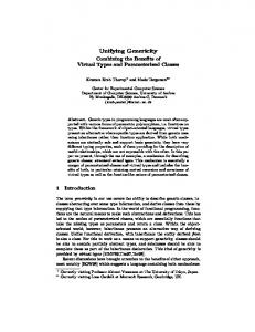
2.1.1 Classical mechanics of a single gyrostat A rigid body containing internal angular momentum, e. g., stemming from an embedded rotating mass, is called a gyrostat [149]. In this section it will be sufficient to rely on the setup in Figure 2.1 showing a gyrostat with several Cartesian frames1) : one inertial reference frame FI , one arbitrary reference frame F0 and three frames fixed to the body, a center of mass frame Fc and two body-fixed frames FA and FB . For the moment the motion is considered unconstrained and free of external forces such as gravitation. The body has constant mass m, a constant inertia dyadic2) w. r. t. Fc c J, and the vector of internal relative 1)

A Cartesian frame in Euclidean space is characterized by the location of its origin O and the orientation of three orthogonal(-normal) axes : e = {e1 , e2 , e3 } forming a dextral system, a vector base. The symbols used throughout this work are Fx or {Ox , x e} to denote location and orientation explicitly. All frames used in this work are Cartesian. R 2) A continuum distribution of mass results in a tensor of moments of inertia c J with matrix components cc J αβ = body ρ(x)· (x2α δαβ − xα xβ ) · dV , α = {1, 2, 3} when resolved w. r. t. a body-fixed basis. ρ(x) is the mass density. The formed matrix is symmetric positive-definite.

10


angular momentum w. r. t. Fc is c l. Please note, that in this work Cartesian tensors of first and second rank are consistently referred to as vector and dyadic, in contrast to m-dimensional matrices, except for matrices ∈ Rm×1 which are referred to as column vectors. Bold typeface 1 x indicates a tensor with a reference point O1 , italic typeface 21 x denotes a matrix representation of 1 x w. r. t. vector basis 2 e. cl c

o

c

I

F IGURE 2.1: Schematic setup of one inertial frame F I , one reference frame F0 and two arbitrary frames FA and FB attached to a gyrostat with center of mass frame F c . Important to note that only FI must be inertial. The tilted cylinder symbolizes the internal angular momentum c l.

The fundamental laws of rigid body motion by Newton and Euler state that the net force F and net torque 3) equal the absolute total time derivatives of its linear and angular momentum I p and I τ on the rigid body L: I dI p , dt dI L = . Iτ dt F =

(2.1) (2.2)

Please note for the vectors I τ , I p, I L the frame FI is used as a reference, which must be an inertial frame. Any tensorial quantity tied to an inertial frame is called absolute. A tensor whose reference is noninertial is called relative. Analogously an absolute derivative is the derivative of a vector calculated w. r. t. to an inertial frame (usually symbolized FI ) . An absolute derivative is denoted by x˙ or dx . A dt derivative calculated w. r. t. an arbitrary noninertial frame F1 (or vector basis 1 e) is called relative [115], apparent [41], or local [49] time derivative. It is further referred to as relative derivative and is denoted ◦ 1 dx by dt . If the vector basis is obvious from the context the circle derivative x is used. A vector’s absolute and relative derivative w. r. t. a frame F1 are related by 1 dx dx = + ω I ,1 × x , dt dt

(2.3)

where ω I ,1 is the absolute angular velocity of frame F1 . The relative time derivative can be viewed as derivation w. r. t. a moving but non-rotating frame. When deriving dynamics equations it is more convenient to choose a reference point other than OI . For a general reference point O0 and using r := rI ,c and s := rI ,0 the Equations 2.1 and 2.2 become F = m¨r , d0 L = 0 τ − m(r − s) × ¨s . dt

(2.4) (2.5)

The most important and compact choice is to use the center of mass as reference point O 0 ≡ Oc which implies (r − s) = 0 and using the well-known relationship between translational momentum and mass 3)

In this work action [115] is used to denote the concepts of force and torque.


11

and angular momentum and inertia tensor [149] to obtain the linear and angular momentum equations p = mv , c L = c Jω + c l , I

(2.6) (2.7)

where ω := ω I ,c is the absolute angular velocity of the body and v = r˙ the absolute velocity of the c = dω the dynamical center of mass. After differentiating (2.6) and (2.7) w. r. t. time and using that dω dt dt equations in terms of velocities are dv , dt c dc l dω + ω × (c Jω + c l) + . cτ = cJ dt dt F = m

(2.8) (2.9)

So far all expressions shown were based on pure coordinate free tensorial notation. A matrix representation is obtained if tensors (arbitrary vector v and dyadic D) are resolved w. r. t. an orthonormal vector basis x e := (x e1 , x e2 , x e3 )T v = D =

v = x vT x e Tx x e Dxe xe

Tx

where x eαx eβ = δαβ are the simple Cartesian metric coefficients and hence x eT x e = I3×3 is just the unit matrix. The orientation of the center of mass frame is given by the direction cosine matrix c e = c RI (t)I e.

2.1.2 Coordinate representations Symbolic manipulation and reformulation of the physical laws (2.1) and (2.2) is possible in tensorial form. A matrix representation of the dynamics equations is optional for symbolic treatment, but mandatory for numerical evaluation and implementation on a digital computer. Three key requisites determine the ways of calculating the dynamics: • reference point O0 used for calculating the dynamics in (2.4) and (2.5) • vector bases required for resolving vectors and dyadics • absolute or relative derivatives The notion of a coordinate representation denotes one certain choice of each of the three categories. Some prominent used in robotics are inertial, body, and absolute representation [49]. In order to indicate that a matrix belongs to a certain representation R a left superscript hRiX is used. The symbol R denotes one particular representation, in this work three are used, namely R ∈ {I, B, A}. The goal of this section is to emphasize the existence and importance of coordinate representations used to formulate dynamics algorithms. The design of a dynamics software architecture must consider coordinate representations to enable consistent code generation, code reuse, and interpretation and exchange of computational results during run-time. The prominent representations mentioned are reviewed shortly below, to introduce expressions which form the basis of a family of multibody formalisms. Though describing the same underlying physics, different representations result in different spatial operators, time derivatives, dynamical equations, and, finally, in different matrices, since the operators will describe quantities at different points in space and w. r. t. to different vector bases. Each approach has distinct advantages and

12


properties concerning symbolic und numerical complexity, computational efficiency, and numerical stability as discussed later in Section 3.1 and 3.2. Studies comparing the influence of coordinate representation on computational efficiency of certain classes of recursive methods can be found in [87, 40, 136, 115]. Unfortunately there exists no uniform notation and choice of coordinate representation in robotics literature to describe mechanical quantities, so this section has to (re-)state clear definitions here. 2.1.2.1 Inertial coordinate representation of dynamics In inertial representation the dynamics is calculated (i) w. r. t. a location O x fixed in the body, (ii) with all tensors resolved w. r. t. inertial system I eT , and (iii) using absolute time derivatives. The advantage of this traditional formulation of the dynamics is that all quantities have a direct physical meaning. For compact symbolic expressions we adopt the spatial notation (not to be confused with spatial representation of Featherstone [40]) similar to that introduced by Rodriguez et al. [117] where matrices ∈ R 6 (two matrices ∈ R3 stacked, called spatial vector) and ∈ R6×6 are used. The most prominent are defined in Table 2.1 on the current page. All tensors are resolved w. r. t. the inertial frame F I , the absolute translational velocity dI is defined by I v I ,c := dt rI ,c . TABLE 2.1: Prominent spatial matrix operators in inertial coordinate representation. Here the center of mass O c is used as reference point.

ω hIi spatial velocity Vc := I I ,c v I I ,c ω I ,c hIi spatial angular velocity Ωc := I 03 τ hIi spatial force fc := Ic F I J 0 3×3 c hIi spatial inertia Mc := 0 I 3×3 mI3×3 L hIi spatial momentum Π c := II cIp l internal spatial momentum hIiΠi c := c 0

I

The momentum equations (2.6) and (2.7) can be written compactly hIi

Πc = hIiMc hIiVc + hIiΠi c .

The dynamical equations (2.8) and (2.9) w. r. t. Fc are as follows hIi ˜ c hIiMc − hIiMc hIiΩ ˜ c hIiVc + hIiΠ ˙ ic . fc = hIiMc hIiV˙c + hIiΩ Proof: Taking the time derivative of (2.10) leads to

˙ c = hIiMc hIiV˙ c + hIiM˙ c hIiVc + hIiΠ ˙ ic . Π

hIi

Comparing this expression to (2.9) shows that I I I I ω × Ic J I ω ω ˜ c J ω − Ic J I ω ˜ Iω hIi ˙ hIi M c Vc = = I . 03 ω ˜ mI3×3 − mI3×3 I ω ˜

(2.10)

(2.11)


13

Here the tilde operator 4) has been introduced to express the vector product by pre-multiplication of an anti-symmetric matrix pe ∈ R3×3 such that p × q = pe · q, p, q ∈ R3   0 −pz py 0 −px  . pe :=  pz (2.12) −py px 0

The six-dimensional complement of (2.12) which operates on spatial vectors is called spatial cross product [66] and defined by e ac e where (2.13) X × Y = XY = e bc + e ad e a 0 c a 3×3 ˜ := X . (2.14) , and Y := with X := eb d b e a ˜ c = diag(I ω ˜ c hIiMc − hIiMc hIiΩ ˜ c )hIiVc leads to the result. Using hIiΩ ˜ , Iω ˜ ) and observing hIiM˙ c hIiVc = (hIiΩ

The two kinds of tilde operators satisfy a number of useful identies which are listed in Appendix B. The dynamics of an arbitrary body-fixed location Ox is as follows: hIi ˜ x + hIiV˜x T hIiMx hIiVx + hIiφT hIiΠ ˙ ic . fx = hIiMx hIiV˙ x + hIiMx hIiΩ (2.15) c,x Proof: The transformations for velocity and torque when changing from body-fixed reference point O y to Ox , where l := ry,x is the vector from Oy to Ox , are [115] ω x = I ωy xτ = y τ − l × xF I

(2.16) (2.17)

vI ,x = vI ,y − l × I ω y xF = y F

These equations reflect that angular velocity is the same in the whole rigid body and that the body accelerates identically as a particle of equivalent mass. These fundamental transformation properties can be expressed by introducing the rigid body transformation operator I3×3 03×3 hIi (2.18) φx,y := −I r˜y,x I3×3 which transforms spatial velocities from Fy to Fx and, when transposed, spatial forces from Fx to Fy , thus writing hIi

Vx = hIiφx,y hIiVy

(2.19)

fy = hIiφTx,y hIifx .

hIi

Because l is constant w. r. t. the body it follows from (2.3) dl = I ω × l. Using (B.8) leads to the important dt operator derivative hIi ˙ ˜ y hIiφx,y − hIiφx,y hIiΩ ˜y . φx,y = hIiΩ (2.20) The spatial inertia transforms similarly to the spatial force hIi

hIi T

hIi

hIi

Mx := φc,x Mc φc,x =

4)

cJ I

− mI ˜l I ˜l mI ˜l −mI ˜l mI3×3

The vector product r = P p × q can be viewed as the double contraction of the total antisymmetric pseudo-tensor ε ijk (Levi-Civita symbol) by ri = jk εijk pj qk so the operator p˜ becomes a single contraction of εijk pj w.r.t. to second index j.

14


where its total time derivative, using (2.20), writes ˜ x hIiMx − hIiMx hIiΩ ˜x . M˙ x := hIiΩ

hIi

Omitting hIi superscripts for brevity, the last required operator identity is ˜ x φ−T Mx Vx −V˜x Mx Vx = φTc,xΩ c,x

(2.21)

which can be shown by multiplication of the matrices and using (B.8) and (B.4). Using Ω c = Ωx and hIi φc,x = hIiφx,c−1 one writes fx

= = (2.20)

=

= = (2.21)

=

φTc,xfc ˙ ic φTc,x Mc V˙ c + M˙ c Vc + Π h n o i h i ˜ x φc,x − φc,x Ω ˜ x Vx + Ω ˜ x Mc − M c Ω ˜ x Vc + Π ˙ ic φTc,x Mc φc,x V˙ x + Ω T T ˜ x Vc − M x Ω ˜ x Vx + φ T Ω ˜ ˜ ˙ Mx V˙ x + φTc,x Mc Ω c,x x Mc Vc − φc,x Mc Ωx Vc + φc,x Πic T ˜ x Vx + φ T Ω ˜ −T ˙ Mx V˙ x − Mx Ω c,x x φc,x Mx Vx + φc,x Πic ˜ x + V˜x Mx Vx + φT Π ˙ Mx V˙ x − Mx Ω c,x ic

(2.15) is one of the key results of this section. It is the starting point when deriving other representations, some discussed below, and serves as a basis when treating multiple rigid bodies. 2.1.2.2 Body representation A more concise notation of the dynamical equations is the body representation [149, 109, 49, 113]. Dynamics is calculated (i) in a body-fixed frame Fx , (ii) where tensors are represented w. r. t. to a bodyfixed frame, usually the same frame Fx , (iii) calculating time derivatives in terms of body-local (relative) derivatives. Matrices belonging to this representation are denoted by a left superscript hBi. In case of a single gyrostat the transition from inertial to body representation is merely done by considering possibly different vector bases when transforming between two body-fixed locations F x and Fy and expressing absolute time derivatives by (body) relative derivatives [2]. The rigid body transformation operator (2.18) now writes x Ry 03×3 hBi φx,y := , (2.22) −x Ry y ˜l x Ry where again l := ry,x . With help of the obvious spatial generalization of (2.3), i. e., ◦ dV ˜ xV =V+Ω dt

(2.23)

the dynamics w. r. t. Fx in body coordinates is ◦

˙ ic . fx = hBiMx hBiV x − hBiV˜xT hBiMx hBiVx + hBiφTc,xhIiΠ

hBi

(2.24)

In further symbolic manipulation it might be useful to decompose the rigid body transformation operator in parts for pure rotation and pure displacement: I3×3 03×3 R 03×3 φR (R) := and φD (l) := 03×3 R − ˜l I3×3


15

so (2.22) goes over into hBiφx,y = φR (x Ry )φD (y l) and (2.18) into hIiφx,y = φD (I l). The strong relation between Lie groups and this body representation of dynamics has been pointed out by Park et al. [109]. Following geometrical arguments in the book of Murray et al. [98], one can show that the rigid body transformation operator is a matrix representation of the adjoint operator Ad on SE(3) and the spatial cross product operator definition in (2.13) is a representation of the ad operator on the corresponding Lie algebra se(3). 2.1.2.3 Absolute representation of dynamics The main idea of this representation is to calculate the dynamics at a point fixed in the inertial frame, so that ¨s becomes zero in (2.5). This is in contrast to inertial and body representation where a point attached to the rigid body was used as reference point. Screw-theory based multibody dynamics was elaborated in the book of Featherstone [40] and related to body representation and Lie group interpretations by Murray et al. [98]. The absolute representation is characterized by (i) using OI , the origin of the inertial frame FI as reference point for dynamics, (ii) applying the same frame to resolve all tensors, and (iii) employing total time derivatives for spatial operators. A spatial operator in absolute representation is denoted by a superscript hAi . It can be obtained from the inertial one using the rigid body transformation operator (2.18). The spatial velocity then is hAi V = hIiφI ,x hIiVx . (2.25) The time derivative of a spatial vector in absolute representation is ◦

X˙ = hAiX + hAiV˜hAiX

hAi

(2.26)

◦

which implicates hAiV˙ = hAiV . The spatial inertia in absolute representation is the spatial inertia w. r. t. the origin of the inertial frame OI hAi M := hIiφTx,I hIiMx hIiφx,I ˜ x − hIiV˜x + hIiΩ ˜ x hIiφ˙ x,I − hIiφ˙ x,I hIiΩ ˜ x ) gives the time derivative of the spatial and exploiting hIiφ˙ x,I = (hIiΩ inertia hAi ˙ M = −hAiV˜ ThAiM − hAiM hAiV˜ . The net force acting on the body is the time derivative of the spatial momentum about the origin of F I which leads to the dynamics in absolute representation ˙ ic . f = hAiM hAiV˙ − hAiV˜ ThAiM hAiV + φTc,I hIiΠ

hAi

(2.27)

One appealing property of the absolute representation is that quantities belonging to different bodies and locations can be related immediately without applying transformations such as (2.22). As shown later this leads to an enormous simplification of symbolic expressions describing multiple bodies. On the other hand the physical interpretation of quantities in absolute representation is not as intuitive as in the inertial one. The only mechanical ’device’ discussed so far was the single gyrostat. Its dynamics in three-dimensional Euclidean space is influenced by the gyrostat’s internal characteristic properties (i) mass, (ii) moments of inertia, and (iii) internal angular momentum. A robot consists of various interacting components with different behaviour and properties. The following section attempts to capture the description and behaviour of such multibody systems in a conceptual and a mathematical way – both prerequisites for a computational robot model.

16


2.2 Paradigm for abstract robot model specification This section shows a generalized way of specifying the robot system’s mechanical properties. This is motivated by the idea that specifiying the properties has a counterpart in the process of establishing the system’s equations, to guide generation and organization of code on a later stage. As a consequence this section does not follow the classical introduction of multibody formalisms and starts from more general considerations. In robotics the starting point for formulating the equations of motion often are mechanical systems composed of links. The notion of a link is very useful when dealing with kinematic chains where a number of material bodies are connected sequentially by holonomic joints. In robotics literature a link represents a body and two locations fixed in the body where adjacent bodies are supposed to be connected by a joint. There are two reasons why often coordinate frames are associated with joint locations. On the one hand the convenient and popular convention according to Denavit and Hartenberg [34] describes how frames can be located in the joints. On the other hand many multibody algorithms can be efficiently formulated in joint reference frames [40]. When taking a closer look there remain some open questions even for the specification of this simple case of chain-structured mechanisms: Is the robot’s base itself a link? Does an endeffector or a payload need two joint locations? How should the bodies be indexed? For simplicity most researchers treat robotic mechanisms uniformly as joint-connected bodies, more precisely pairs of one adjacent joint and one body. They assign special meaning to, e. g., link 0 which is treated as the reference system, or introduce specific and context-depending rulesfor model interpretation, or zero-mass or zero-length links. This is very convenient and is an appropriate representation if one stays within one single formalism. But relying on different paradigms and implicit assumptions is awkward for formalism transfer, efficient code generation, and coupling between several algorithms. One example are the algorithms presented in [67], where the crucial information which coordinate representation is used is implicitly contained in the mathematical formalism. Some situations limiting flexibility and applicability of the existing formalisms, such as SOA formulation, to more general multibody systems are: • there are more or less than two frames associated with bodies • the need for MBS topologies such as tree-structures and loops • presence of general entities and physical effects in the system such as internal and external forces, internal angular momentum, or artificial muscles in biomechanics • environmental conditions, such as cooperating robots, inhomogeneous gravitational fields, or boyancy In order to obtain a sufficiently general system model this section tries to answer the questions: • What are the major components of the mechanical robot model? • What is its static and dynamic behaviour? A proven method to achieve the required flexiblity for a modeling language is to model the language itself by an abstract higher-level formalism. Tools that support that kind of meta-formalism are D OME [55] or ATO M3 by Vangheluwe and de Lara [143]. Having an object-oriented implementation at a later stage in mind the following section starts from an abstract level. We generalize from a purely data-driven to an

2.2. PARADIGM FOR ABSTRACT ROBOT MODEL SPECIFICATION

17

abstract model specification by formally capturing the structure of a robot model to handle more complex systems and maintain extensibility. The shown appoach is similar to the P SPEC approach proposed by Hatley and Pirbhai [51] for real-time system specification which contains all the information necessary for the designer to know what to do without saying how to do it. The entity-relationship (ER) model introduced by Chen [26] is applied to formulate the parts of a mechanical robot model in a component-oriented and port-based way. This concept of a component is denoted by MBS entity. Components and contexts known from robot and multibody system dynamics are analyzed w. r. t. to the MBS entity paradigm to capture and classify the behaviour and all concerned relevant information and relations. The advantage of this approach is an abstract high-level view on the properties of the components and relations between the parts revealing explicitly as much information as possible without doing, e. g., a simulation run. By this the following ameliorations are attained: • Efficient code generation for various algorithms, e. g., according to a dataflow model of computation, may be based on different assumptions about the model. These can be expressed explicitly and are not entangled within code or a mathematical formalism. • Enhancing the potential for optimization of the given model description according to different criteria. • Dynamics computations might not be the only software task to be driven by a robot specification in a robot control system, so the reduction to just links limits the applicability of the model. Integration of components, implemented by persons with different objective and background, is enabled because created objects are based on the same reference model. • Checking for model correctness by formal methods. • Clear textual or graphical representations enabling persistence of model description and system state. • When formulating mathematical equations by means of spatial operators introduced in Section 2.3 and defining topology and causality of the multibody model graph the ER paradigm is beneficial. The goal is to preserve the advantageous algebraic properties and explicitness of spatial operators expressing physical properties directly.

2.2.1 Component specification model Multibody systems such as robots naturally offer a component-oriented view for two reasons. On the one hand real mechanisms consist of distinct rigid bodies, joints, force-element, drives and other devices. Problems from biomechanics also allow such a subdivision into bones, muscles, tendons. On the other hand the mathematical equations describing these systems show a similar structure which is exploited by dynamics formalisms, which will be shown in Section 3.1. As discussed above researchers often reduce this set of components to one member, the link, e. g., see [60], or restrict their properties for specification of the robot in order to formulate, e. g., dynamics algorithms for that class of components. This procedure is completely legitim, but one might run into problems to drive several algorithms by one single specification, because assumptions about the behaviour of components were made implicitly. Basing the components’ description on an abstract representation which captures formally all properties and behaviour and their relations is the solution proposed in this section. 5) 5)

This section is an advanced version of parts of the paper [56].

18


The entity-relationship (ER) model [26] offers in a natural way an abstract view on systems primarily formed by components. The concept is based on the general idea to represent the data in two logical parts, entities and relations. An entity e is defined as a ’thing’ which can be distinctly identified, a relationship r is an association between two entities. Both can be augmented by attributes, which may represent arbitrary data. Entities are classified into different entity sets Ei . There exists a predicate associated with each entity set to test whether an entity ei belongs to it. A relationship set Ri is a mathematical relation among n entities, each taken from an entity set {[e1 , . . . , en ] |ei ∈ Ei } and each tuple [e1 , . . . , en ] is a relationship. A graphical representation for ER models is offered through ER diagrams. In this work the relations between concrete realizations of MBS entities, objects, are graphically represented by Unified Modeling Language (UML) [100, 101, 127] class diagrams, where an entity is represented by a UML class symbol and a relation by a UML association symbol. The UML is a mainly graphical notation or syntax that object-oriented methods use to express software designs. The portions of the UML applied in this work relies on the presentation in [43]. Figure 2.2 shows the graphical constructs used in this section. ER diagrams are expressed here using UML class diagrams which describe the types of entities in a model and the various static relationships that exist between them. The two principal kinds of static relationships between classes are association and subtype. A class is depicted by a rectangular box. The association represents a conceptual relationship classes. It has two ends, which can be explicitly named by a label called role name. It has a multiplicity, which is an indication of how many objects may participate on each end in the given relationship. Multiplicity can be a whole number or a range denoted by x..y, x, y ∈ N, and * denotes an infinite number. On a less conceptual level a class may have a number of attributes and operations listed in separate blocks inside the box. From a conceptual perspective attributes are like associations, the difference shows up in the implementation perspective not considered here. Operations are the processes that a class knows to carry out. The composition expresses that a part belongs one whole, the class where the line ends in a black diamond. The dependency among components show how changes to one component may cause the depending components to change. The generalization of Supertype to Subtype states that Subtype1 is a subtype of Supertype, i. e., an extension where attributes of the supertype are replicated and new ones can be added and operations of the supertype may be either replicated or overridden by new operations. Association

Class/Object Class

Class

Class B

Class A role A

attribute : type

role B

Composition

operation(arglist: void) : type Class A

object name:Class Name

Class B

Dependency Generalization

Class A

Class B

Supertype

Multiplicities

Class

0..1

Class

0..*

Note

Subtype1

Subtype2

F IGURE 2.2: Groups of graphical constructs used in UML class diagrams, required to express Entity-Relationship (ER) diagrams. For the interpretation of the constructs please see text. Right side: A is associated to B, B is composed of A, B depends on A.

The first step in the design of an ER model of robotic mechanisms is to identify the entity sets and rela-


19

tionship sets which are necessary. The analysis performed in Section 2.1.1 suggests to base the component model, visualized in Figure 2.3, on the following entity sets which graphically are expressed by the UML symbol for a Class: • MBS entity (ME) • Interaction port (IP) • Physical state (PS) • Physical property (PP) • Coordinate Frame (CF) • Constraint Relations (CR) The components from the multibody and robotics domain are subsumed under the entity set MBS entity (ME). The robot and parts of its environment are restricted to be constructed from a finite set of primitive domain components that is sufficient to cover a large class of robots, either representing technical devices or physical phenomena: • joints (revolute, prismatic, etc.) • rigid links and bodies • spring, dampers, and external forces • drivetrains • mechanical unilateral contact • custom-specific or more abstract parts An analysis based on the ER model for a selected number of fundamental components including their substructure is given in the following sections. The MBS entities and attributes are indicated by a different typesetting, using sans serif. MBS entities are supposed to interact via distinct interaction units called interaction ports (IP). The kind of interaction is not specified on this abstract conceptual level. Concrete examples are mechanical connections, e. g., fixed, unilateral contact, or interaction that may takes place on a pure logical level. Context dependent port semantics will be applied to determine the interpretation of a port. In mechanics a body denotes an entity carrying mass and mostly having a geometrical extension. So each ME is related to some physical property, such as mass, angular momentum, etc., which are captured by the entity set physical property (PP). PPs are time-independent in a physical sense which distinguishes them from physical state (PS) attributes. These represent state information, e. g., joint angles, forces, etc. As shown in Section 2.1.1 in multibody dynamics most physical phenomena such as force and torque, are of tensorial nature. Tensors often are inherently related to reference frames and require coordinate frames to be resolved in matrix form. Though coordinate frames are an idea of geometric nature, these are of such fundamental interest in MBS dynamics to motivate the entity set of coordinate frames (CF). The substructure of an ME represented by the attributive entity sets IP, PP, PS, and CF, is related by composition relationships. This idea from object-oriented modeling can express well that, e. g., the idea of

20


a mass value without any related body is of limited physical sense in a robot model. Optionally, the PP can depend on each other. The constraint relationship set models this dependence which might be (i) a mutual dependency, e. g., mass and moments of inertia can be calculated from geometrical shape and mass density of a body (see footnote on page 9), (ii) parameter values may restrict the range of other parameters in order to get a physically meaningful model, e. g., requiring the matrix of moments of inertia being positive definite. Both relations may be expressed for instance by symbolic expressions. Some PP such as inertia matrix require the existence of a reference point or frame to be meaningful. This reference relationship set expresses that a PP has a discrete number of reference frames. In a numerical computation the components of vectors and tensors must be resolved w. r. t. a vector basis (see 2.1.2) to obtain numerical values. The relationship set representation states which vector bases are used to represent the matrix entries. More generally speaking, this allows for interpretation of the model specification but not determines physical reality. IP entities are supposed to represent the points where ME entities can interact. When dealing with mechanical interaction, inevitably a location in space is required to define where the interaction takes place. In numerical schemes a complete coordinate frame CF is required to resolves vectors. The association between a CF and IP entity manifests this. Note that not each CF has to be associated to an IP because reference frames might not be ’exposed’ to the outside of a component and may remain a conceptual idea required on a logical level. The relationship set defined on the single entity set ME is the component relation. This relation models the hierarchical decomposition of entities into parts. If cardinality is greater than zero such an ME is referred to as MBS assembly. A component relation might induce some additional constraints on the structure of an ME which are discussed below. In this conceptual view, it is not mandatory to apply another feature of the ER model, attributes and associated value sets representing any kind of data belonging to entities and relationships. Concrete examples forming the basic classes for a robotics domain component library are given in the next section where entities of the multibody domain are modelled using Figure 2.3. In the first step properties are emphasized, resulting in an abstract data model, and in the second step emphasis is on behaviour (transformation model). 0..*

Physical property 0..* Representation 0..1

ConstraintRelation

0..1

Reference 0..1

Coordinate Frames

Interaction Port

MBS entity 1..*

2..* Representation

Reference

0..* Physical State 0..* MBS Context

0..* MBS Connection

F IGURE 2.3: Conceptual Entity-Relationship model of an MBS entity and its constituents in graphical UML notation.

2.2.1.1 RigidBody entity In mechanics a body denotes an entity carrying mass, having a geometrical extension, and locations where some actions can be applied. In the domain of multibody system dynamics one can take the attributes mass


21

m and inertia J for granted. The nature of a body is the ability to couple to a gravitational field and to react to external action by inertial forces as discussed in 2.1.1. The interesting thing is, that even this well-accepted view is implicitly based on modeling assumptions. Considering the gravitational (volume) forces these properties are only sufficient to some extent to calculate the dynamics correctly. Only for homogeneous fields the center of mass, which is the point upon the net inertial forces act, is identical to the center of gravity, onto which the net gravitational volume force acts. So without further semantical information stemming from some kind of context and some additional physical information about the mass distribution of the body this model is valid for homogeneous fields. 6) Modeling these concepts within the MBS entity paradigm yields Figure 2.4. The most general model RigidBody contains physical property attributes denoted by PP:mass and PP:inertia. The latter requires a reference point and a vector base represented by CF:Rep and CF:Rep. There are a number of N F frames CF for designating locations attached to the body which are exposed to the same number of interaction ports IP:x. The constraint relation between the frames CF:Ref and CF:x might be implicit or explicit. If one identifies CF:Ref with the center of mass system this is a MBS entity model of the body depicted in

Figure 2.1 for NF = 2. PP:mass

PP:Inertia 0..1

CF:Ref representation

IP:x

ME:RigidBody 1..*

position constraint

position constraint CF:Rep

CF:x

F IGURE 2.4: ER model of the MBS entity RigidBody.

The most concise specialization of this model is MBS entity RigidBody, which is shown in Figure 2.5. It represents a body with one interaction port called IP:1 and one frame F CF :1 represented by CF:1 associated with it. This component can only act as a leaf in a multibody graph structure. The reference system of the inertia PP:I is the center of mass frame CF:CM located in the center of mass and equivalent to FCF :1 . The vector basis used to represent the entries of J is also 1 e. The specialization tag denotes the number of frames NF = 1 and Type1 the equivalence of the center of mass frame and FCF :1 . PP:Inertia I11 : double I22 : double I33 : double

PP:mass

reference

m : double

CF:CM

I21 : double

representation equivalence

I31 : double

CF:1

IP:1

ME:RigidBody

I32 : double

F IGURE 2.5: ER model of the specialized MBS entity RigidBody. 6)

Hence, this assumption holds for all ground-based robots and technical processes, but not for geostationary satellites of large extent.

22


From Figure 2.4 the mathematical operators as discussed in Section 2.1.1 can be extracted. From the viewpoint of a mathematical formalism using spatial notation the proposed rigid body provides a spatial inertia matrix MCF w. r. t. a frame FCF and rigid body transformations φCF :x,CF :y between various frames where x 6= y, x, y ∈ {1, . . . , NF } , where the set {FCF :1 , . . .} must be exposed by the interaction ports. This is one kind of behavioural description of a rigid body. To provide more modeling flexibility it should be possible to derive models which provide a different view [38] on the body data, e. g., to supply information about the mass density and geometrical data. The number of PP will increase, and due to the redundancy some constraints for deriving the body data has to be provided. The only difference is in the data model. It must be emphasized, however, that such a component must have the same behaviour as a rigid body otherwise it would represent a different entity. To capture this fact by the modeling paradigm is exactly the reason to take this abstract point of view. It should be noted that the model chosen above is motivated by separating the characteristics of the rigid body. A more user-friendly specialization of the RigidBody entity should provide attachment points different from the center of mass.

2.2.1.2 Displacement entity Describing one reference location O1 on a rigid body by means of a second one O2 on this body, often required in robotics, implies a time-invariant shift between two locations by a vector r 1,2 . In mechanics terms this behaviour shifts an attachment or reference point or the point of application of actions to a different location. Introducing two coordinate frames F1 and F2 there also is the possibility to change the local vector basis 2 e = 2 R1 1 e which does not affect the physical behaviour of shifting the reference point. This behaviour offers several interpretations depending on the modeling concepts used ranging from massless rigid rod or rigid body to homogeneous transformation or a link with zero degree of freedom. Mathematically spoken, a displacement entity puts a positional constraint between two coordinate frames which depends on time-invariant local positional parameters. Figure 2.6 shows an ME diagram of that dependencies. CF:1

IP:1 Displacement

PositionConstraint CF:2

IP:2

F IGURE 2.6: ER model of the MBS entity Displacement.

The positional parameters denote a set of time-independent parameters describing how the relative translation and orientation between the two frames CF:1 and CF:2 is parametrized. The most common used in robotics are Denavit-Hartenberg (DH) parameters [34] and related sets by Craig [29] and Khalil and Kleinfinger [76] and separate parameterizations of translation and rotation, e. g., through Euler-angles or quaternions [98]. A model of a simple displacement is shown in Figure 2.7, which represents a simple translation parametrized by matrix CF :1 rCF :1,CF :2 . This is referred to as Displacement and equivalent to the component called ’FrameTranslation’ in [94]. Extracting mathematical operators from the model described in Figure 2.6 shows a behaviour which is very simple in terms of spatial operators. The operator concerned by this kind of ME is the rigid body transformation operator φCF :1,CF :2 through positional constraint.


PositionConstraint r : Vector3

CF:1

23

IP:1 Displacement

CF:2

IP:2

F IGURE 2.7: ER model of the specialized MBS entity Displacement.

2.2.1.3 Joint entity Constrained motion between two bodies results (i) from direct physical contact of two bodies or (ii) from an interconnection of two bodies by means of kinematically constraining mechanisms, whose mass and inertial properties have been lumped with the bodies connected. Important examples often applied in mechanical engineering are revolute, prismatic, universal, and ball joints. It is possible to model the effects of rigid body contact and a constraining mechanism as two coordinate frames F 1 and F2 whose relative motion is kinematically constrained and the contiguous bodies are thought to be attached w. r. t. to the two frames. In both cases (i) and (ii) the idea of the kinematic equality constraint as a separate entity is called a joint. Situations where more than two points or frames have to be contrained at once or the constraint must be expressed in terms of an inequality relation is rarely encountered in robotics and are not investigated in this work. The ideas developed in this section are based on the general mathematical treatment of representations of joints in multibody systems by Schwertassek and Senger [124]. The fundamental characteristic to distinguish the behaviour of joints is the way they relate the relative motion of frames F1 and F2 . Unconstrained motion between two frames has 6 degrees of freedom (dof), i. e., one requires 6 independent variables to describe the relative position 7) . The set of independent variables parametrizing the relative position and velocity are generally called position and velocity state variables denoted by symbols qp and qv . The number of holonomic and nonholonomic constraint equations be N f p and Nf g . The number of motional dof Nf across the joint then is Nf p + Nf g = 6 − Nf . It has been pointed out in [124] that using relative position and velocity variables allows for all constraint equations to be established without any knowledge about the multibody aspects of the whole system under consideration. This enables a completely component oriented view on every type of joint with a minimum coupling to the complete model. The various joint types can be compiled in an independent joint library which allows for changes in the applied multibody formalism without requiring changes in the library. That perfectly fits into an object-oriented modeling paradigm with demand for encapsulation and minimum but well-defined coupling between all parts of the system. The main characteristic of joint behaviour is captured by a classification of the type of its positional constraint. From a data perspective the requirements for the description of a joint in a multibody dynamics simulation are • joint positional constraint (desirable in mathematical explicit form), • sets of joint position state variables qp and joint velocity state variables qv , • kinematical equations of motion, i. e., the relations between the chosen velocity variables and the time derivatives of the position variables, • mode vectors and dual vectors, describing the mappings between state space in cartesian space. There are two more categories given in the joint description [124] not considered in this context for clarity. The first are so-called kinematical excitation functions which describe modes of motion which not excited 7)

Position encompasses the terms displacement and orientation.

24


by state variables. This feature of special mechanisms is not required in robotic applications. The second are laws for the generalized applied forces, i. e., functions representing applied interaction forces in terms of the motion across joint most prominently friction, which is later captured by drivetrains including friction. KinematicConstraint PP:DualVector CF:2

CF:1

IP:2

IP:1

PP:ModeVector

constraining PS:JointStateVar

IP:3

Kinematic eom

ME:Joint

F IGURE 2.8: ER model of the MBS entity Joint.

In the domain of robotics the most important joints are revolute and prismatic which are single dof joints. They constrain the motion between frame F1 and F2 along one axis n. One obvious choice for relative ˙ The kinematical position and velocity state variables are the joint angle θ and its time derivative θ. d equations of motion take the most simple form qv = dt qp . One concrete specialization is shown in Figure 2.9 and called Joint. The classifier Type1 denotes the parameterization of the positional constraint equation, in this case using an arbitrary axis of rotation resolved w. r. t. frame F CF :1 hence CF :1 n. PP:ModeVector

PositionConstraint

n : Vector3 representation

PS:Angle CF:1

CF:2

IP:1

IP:2

CF:3 IP:3

Joint

F IGURE 2.9: ER model of the MBS entity Joint.

The spatial operator induced by the positional constraint is the rigid body transformation operator φ CF :1,CF :2. A crucial point for all algorithms based on a joint space or state space representation – actually the most efficient ones – is a mapping between the spaces of velocity variables and cartesian velocities and its dual mapping between cartesian actions and variables of generalized force variables. In the simplest case of single dof revolute joints this turns out to be the mappings between joint angular velocities and torques and cartesian velocities and actions. In case of holonomic constraints the mode vectors and its dual are equivalent to the joint projection operator H [66]. This operator will be applied in the further analysis in the following sections. If CF :1 n is a unit column vector describing the axis of rotation of a revolute joint T T the H = (CF :1 n , 0T3 )T , if CF :1 n is the joint axis of a prismatic joint H = (0T3 , CF :1 n )T .


25

2.2.1.4 ReferenceFrame entity Motion of mechanical systems finally are described w. r. t. inertial space. The idea of a reference frame component is a coordinate frame whose translation and orientation w. r. t. an inertial frame are known functions of time, which may, in particular, be zero [115]. This frame could be reference to one prominent (’reference’ or ’main’) body attached to the robot mechanism, and is strictly speaking not a part of the mechanism itself. Or one might choose a reference frame corresponding to no material body and having no physical relation with any body of the system. This case can be covered by the idea of a ’conceptual’ joint relating the reference frame and the ’main’ body. Because this conceptual joint models, depending on context context, different qualities from a ’real’ joint entity [115] it is part of the separate ReferenceFrame model shown in Figure 2.10(a). For instance a conceptual joint with six degrees of freedom [40] does not constrain motion in any sense. ReferenceFrame is a purely kinematical concept, though similar components, as reported in literature [94], carry semantical information about gravitional acceleration. As discussed in Section 2.1.1 this implicitly assumes a homogeneous gravitational field. More important is the meaning of ReferenceFrame as part of the description of the robot’s environment. Information is required on which parts of the robot model are interacting with, e. g., the ground if it is mounted on the floor. The specialized model ReferenceFrame shown in Figure 2.10(b) is designed to express these conditions. The specialization tag tells that the frame is a kinematic reference where the inertial frame coincides with the frame of reference. CF:InertialFrame

CR:PositionConstraint

CF:1

equivalence CF:InertialFrame PS:PositionVariable

CF:1

IP:1

IP:1

ReferenceFrame

ReferenceFrame

(a)

F IGURE 2.10: Left: ER model of ReferenceFrame.

(b)

the

MBS

entity

ReferenceFrame

and

its

specialization

2.2.1.5 Default component set and additional components Robotics is a rapidly developing domain with a vast range of applications. Vew types of components and machines are continuously emerging and there is undoubtedly an increasing demand for precision, safety, and efficiency. This is reflected by the modeling requirements where domain specific solutions and new algorithms require new types of components catching more detailed physical effects. In Section 3.2 where algorithms for concrete applications are presented some more types of specialized MBS entities will be introduced, e. g., representing elasticity, physical contact, or angular momentum. When considering the Multibody entities in the following chapters, prominently in the context of multibody system algorithms we will rely on a default set of components which are listed in Table 2.2. These suffice to describe tree-structured robot mechanisms system with fixed base on a detailed level without further assumptions. The table also introduces an iconic representation für each default entity useful

26


in drawing multibody component diagrams and shows which spatial operators appears in the equations through the presence of this type of entity in the model description. TABLE 2.2: Default set of MBS entities.

MBS entity declarator

iconic representation

ReferenceFrame

spatial operator

1

RF

3

Joint

Displacement

RigidBody

1

2

H,Φ

2

Φ

JR

1

D

1

RB

M

2.2.2 Robot specification model Known interconnection topologies of the robots are: • kinematic chain • star topology • tree structure • partial loops • fully closed kinematic mechanisms Figure 2.11 shows a schematic view of each class of these mechanisms. When mechanisms are depicted schematically throughout this work, small circles symbolize any kind of holonomic joint and ellipses material bodies. The reason to do this subdivision is that each class has distinct mechanical properties and hence algebraical properties in a mathematical description. For instance the presence of kinematic loops make the numerical treatment of kinematics and dynamics much more intricate due to additional algebraic constraint equations. One main issue of the various existing dynamics formalisms in general and one main topic of this work is to exploit this structural properties to arrive at an efficient numerical representation of the governing equations. The most common type of mechanism in robotics is the kinematic chain, a series of bodies, where adjacent ones are connected by joints. There is one body with a special status lying on one end of the chain which is called reference body, or robot base. When several branches emerge from one common reference body the system has star topology. When branches are allowed to emerge from every body in the system, the mechanism is called to have tree structure. In a tree the total number of joints N J + is one less than the total


1

1

(a)

(b)

27

1

(c)

(d)

(e)

F IGURE 2.11: The main topologies of robotic mechanisms depicted schematically. From left to right: chain structure, star topology, tree structure, partial loops, and fully closed mechanism.

number of bodies NB + . Index + denotes numbers which are related to the multibody system as a whole. Introducing some additional joints which connect some of the branches of the tree leads to kinematic loops, each extra joint forming one loop. When each body is at least connected to two contiguous bodies by joints the robotic mechanism is called fully closed. Most robots belong to the class of moderately constrained mechanical systems, i. e., the number of mechanical degrees of freedom of the robot equals roughly the total number of bodies and the total number of mechanical dof and the number of kinematic loops is low in comparison to the number of bodies. Model component interaction is based on a port concept in this thesis, a versatile technique from objectoriented modeling that is sufficiently powerful to handle the MBS domain. Relations between MBS entity objects are established by an MBS connection (MC) between two or more interaction ports. The interpretation of an MBS connection is manifold and depends on the level of abstraction one is considering: • From a modeling perspective it is an undirected relation between two or more interaction ports. It can be represented by pairwise binary relations or by relations between multiple ports. To reduce modeling errors it is possible to enforce or avoid the formation of topological constructs by restricting the possible connections. This has been used, e. g., in [104, 56] to enforce the formation of a spanning tree of the model graph by providing two complementary types of ports, A- and B-types, allowing only for connections between one A- and one B-port. This strategy is adequate if the application relies on tree-structure only. The limited scope of the application, for instance a dynamics algorithm for tree-structure, is mirrored in the modeling paradigm. In this work assuring, if the topology is adequate for a certain application, is postponed to a later logical stage where information is available about the requirements from the algorithm to apply. • From an MBS perspective it defines a unique location or frame where two or more entities of the MBS model interact mainly mechanically. Depending on port semantics and the type of coordinate frame associated to the interaction port, this corresponds to different levels of detail in physical modeling. One encounteres two types in this work. The first is a fixed mechanical connection in a spatial frame living in three dimensional Cartesian space. This can be illustrated by matching all coordinate frames associated to the ports taking part in the MBS connection in one frame. The second is used for drivetrains where the associated coordinate frames are aligned along a conceptual symmetry axis.

28

CHAPTER 2. MODELING ROBOTS • From an implementation perspective kinematic and dynamic data which are exchanged between the components, e. g., force and torque vectors, are represented and available in coordinate frames associated to the ’implemented ports’. This concept is borrowed from the concept of ’cut’ actions in mechanics, two examples for this perspective are the works of Leister [85], Kecskeméthy [74]. In the dataflow model presented in the next section a re–interpretation of a multiple relation between N ports to a (tree-structured) set of directed connections is mandatory to result in streams of welldefined input-output causality of the software components representing the MBS entities and their ports.

2.3 Relating recursive dynamics algorithms to dataflow This section relates the important class of efficient and versatile recursive multibody algorithms to the model of dataflow. This has two advantages: First, the algorithm for a complete robot can be established symbolically from properties and equations describing the components and their interconnection structure. Second, the dataflow model of computation allows for an immediate conversion of the algorithm into code or an executable. In multibody view a robot is an ensemble of material bodies connected by joints, including some interactions through actuators, elastic elements and external forces such as gravitation. Such systems can be treated mathematically and numerically by a number of formalisms. Modeling a technical system by means of a network of operators or blocks transformings flows of data is well known from the domains of electronic circuits and automatic control. A higher-level description is achieved by using transfer functions with block-diagram structures and the dynamical equations capturing the behaviour of the systems. These formalisms are rather similar to what a dataflow system is in the domain of computer science [71, 84]. The P TOLEMY project [23], for instance, studies modeling, simulation, and design of concurrent, real-time, embedded systems. The focus is on assembly of concurrent components. The key underlying principle in the project is the use of well-defined models of computation that govern the interaction between components. A major problem area being addressed is the use of heterogeneous mixtures of models of computation. Model-Integrated Computing [138] has been developed for building embedded software systems. The key element of this approach is the extension of the scope and usage of models such that they form the "backbone" of a model-integrated system development process. The main application domain is signal processing. The family of recursive multibody formalisms stresses transformation properties of each component and topological properties of the system as a whole. Starting from this observation this section develops a symbolic mathematical representation of multibody systems such as robots which combines information about interconnection structure and equations describing the components. For reasons that become clear in the following this mathematical representation is called Port-Based Spatial Operator Algebra (PSOA). There are distinct advantages of using the dataflow model as a basis for a high-level description which are discussed in [47]. It is a functional model with its subsequent mathematical representation, with no complex side effects, amenable to formal verification and safe program transformation, because functional relations over dataflows might be time invariant properties. Moreover it is an inherent parallel model, where any sequencing and synchronization constraints arise from data dependencies. The following section develops mathematical operators for the description of multibody system dynamics within the high-level dataflow paradigm.

2.3. RELATING RECURSIVE DYNAMICS ALGORITHMS TO DATAFLOW

29

Port-Based Spatial Operator Algebra The formalism developed in this section can be viewed as a natural extension of the Spatial Operator Algebra (SOA) introduced by Rodriguez et al. [117]. PSOA extensions (a) offer a more general way to specify and describe mechanisms and (b) alleviate development and object-oriented realization of recursive symbolic multibody algorithms which are applicable to a broad range of robots [63, 68, 65, 66, 67]. As revealed in Section 2.1.1 even the mathematical description of one single body requires considerable algebraical effort. The spatial operators and operator identities derived through SOA help in reducing the symbolic complexity and arriving at more concise expressions. Spatial operators present powerful means to establish spatial recursions, i. e., to state the kinematics and dynamics equations of complex rigid multibody systems symbolically and recursively. The following sections clarifie the relation between MBS model structure and spatial recursions, i. e., the entities that are to be modeled and the algebraical relationships between them. The idea is that a generalized way of specifying the mechanical system’s properties has a counterpart in the process of establishing the system’s equations, to guide generation and organization of code on a later stage. As a consequence this section does not follow the classical introduction of multibody formalisms and starts from more abstract arguments. Multibody component diagrams Consider an N-joint kinematic chain with fixed base, the case N = 2 being depicted schematically in Figure 2.12(a). Following robotics literature, bodies are numbered ascending from 0, where index 0 denotes the robot base. Starting from body 0, the joint labelled i is followed by body labelled i. Moving from base body to bodies/joints of increasing index is called outboard direction, the opposite direction is called inboard. 0

1

1

2

2

1

2

L0

(a)

1

RS

3

L1

4

5

L2

(b)

3 4

2

11

7 8

6

5

JR2

D1

JR1

9 10

D2

RB2

12 13

D1b

RB1

(c)

F IGURE 2.12: (a) Schematic view of a tooled 2-joint kinematic chain manipulator and (b) a more abstract graphical representation, (c) a more detailed representation using the default MBS entities from Section 2.2.1.5. Outlined boxes are MBS entities, black squares MBS ports indexed starting from 1, straight lines between ports are MBS connections.

A graphical representation of Figure 2.12(a) where the interconnection structure is more emphasized are shown in Figure 2.12(b) and (c). Joint i and body i and their mechanical connection are merged into a

30


single component represented by an outlined box. The mechanical connection between joint i and body i−1 is symbolized by a straight line terminated by black squares placed on the boxes’ border. The compact iconic representation is taken from [127] where it is used to draw Unified Modeling Language (UML) class collaboration diagrams [100] in order to explicitly represent interconnections between architectural entities. At this stage it is sufficient to mention that in [127] outlined boxes represent capsules, black squares ports, two ports connected by a line a connector. We will further refer to such a diagram as MBS component diagram (MCD). The outlined and filled boxes in a MCD are iconic representations of MBS entities and MBS ports. The straight line between two connectors represents a MBS connection. The rules for drawing a MCD are defined as follows: (i) An MBS entity owns one or more ports which lie on the boundary. (ii) An MBS entity may contain an arbitrary number of other MBS entities. (iii) Ports must belong to any MBS entity and lie on its border. (iv) Connections terminate in ports, nowhere else. (v) Connections are irreflexive, they relate two different ports. Self-connections are not allowed. (vi) Connections are transitive, if port 1 is connected to ports 2 and 3, then there is a connection between 2 and 3. This rule might not be explicit in the MCD. (vii) Two different ports may be related by exactly one connection. No parallel connections are possible. These rules induce a transitive binary symmetric relation on the ordered set of ports. The interconnection structure of an ensemble of MBS entities is captured by the connectivity matrix which is introduced here. This matrix determines which pairs of ports are coupled by a connection. Each of all N p ports, which are present in a MCD, are assigned a unique integer value {1, . . . , N p }, as shown in Figure 2.12(b). Identifying this value with a component index the connectivity matrix C ∈ F Np ×Np is defined by ( Ci,j = 1, if there is a connection between port i to j, (2.28) C := Ci,j = 0, otherwise, where F is the set of numbers {0, 1} with addition and multiplication modulo 2. C is inherently symmetric as the relation ’connection’ is symmetric and all diagonal elements are zero because of rule (v). Ports which are not connected are open and lead to zero colums/rows in C. Roberson and Wittenburg introduced a graph theoretical description of multibody systems [116, 149]. A comprehensive overview of applications of graph theory in MBS dynamics can be found in [115]. Some required definitions and properties are reproduced here. A graph G(N, E) is defined as the nonempty set of nodes (or vertices) N and a set E of pairs of these nodes, called edges. If the set E is ordered one can assign a direction to each edge and the edges and the graph are called directed. Otherwise the graph is called undirected. We are concerned with graphs that are simple, i. e., that contain no self-loops and multiple edges and which are connected. If ports are omitted from the MCD and each entity and its ports are represented by one node one obtains a connected graph G. Undirected graph edges represent connections. The connectivity C + of the graph is obtained from the connectivity of the MCD using the port-entity projection operator P E ∈ F Np ×Ne defined by ( P Ei,j = 1, if port i belongs to entity j, P E := P Ei,j = 0, otherwise

2.3. RELATING RECURSIVE DYNAMICS ALGORITHMS TO DATAFLOW

31

which requires a sequential numbering of the nodes starting from 1. P E can be used to collapse C to get C + := P E T · C · P E. C + determines connectivity between MBS entities and not between ports. Causality and spatial recursions Starting from the visual syntax of the MCD we are now able to specify a graphical description resulting in a directed graph where nodes represent entities from the multibody domain and edges represent a mechanical interrelation. Turning to recursive multibody computations, either symbolic or numerical, the notion of a dataflow process network [84] becomes valuable, where nodes represent transformations and edges directed streams of data, in MBS domain: usual kinematical and dynamical values. The first step is to refine the connectivity by assigning a direction to all connections. Thus each port is represented by a unit vector ui ∈ FNp , i ∈ 1, . . . , Np and either defined to be outport or inport. A directed connection points from one outport to one inport. The unit vectors of all outports form the columns of the matrix O and span the outport space and those of all inports form I and span the inport space. {O|I} forms a complete basis of the linear vector space FNp , if each port is either defined in- or outport. For example, the MCD from Figure 2.12, if ports 0, 2, 4 are defined outports, results in 

0 1  1 0  0 1 C=   1 0

 0



    , O =     

1 0 0 0 0

0 0 1 0 0

0 0 0 0 1





     , and I =     

0 1 0 0 0

0 0 0 1 0



  .  

Proceeding from this pure topological considerations the next step adds new connection semantics and defines which dataflow quantity8) is used and transferred between MBS ports. As a first example we choose the spatial velocity V ∈ R6 and associate one vector to each of the Np ports. The Np velocities are stacked to form the stacked spatial velocity V ∈ R6Np . The ith spatial component vector of any stacked vector is denoted by right lower index V[i] ≡ Vi in square brackets. In order to state transformation properties of the MBS entities we add new port semantics and associate a frame Fi in Euclidean space with each port i. In our example obviously F 1 ≡ FI and F5 ≡ FNp is the tool frame. The semantics of an MBS entity now is to transform data entering from all the inports to all outports. For the moment it suffices to think of a linear transformation similar to (2.19). A good example to explain the transformation property between ports are 2-port MBS entities representing the coupled joint-body pair from Figure 2.12, where i is the port at the joint side and i + 1 the port on the body side. The spatial velocities of frames Fi and Fi+1 associated to the ports, V[i] and V[i+1] are related by V[i+1] = φi+1,i V[i] + ∆i+1 . (2.29) The relative rate of velocity change across the joint ∆i+1 depends on the inner properties of the MBS entity, e. g., the joint angle q. The spatial velocity V [i] transforms under the rigid body transformation operator φi+1,i analogously to (2.19). Please note that the expressions derived are independent of coordinate representation R, thus index hRi is omitted. The rigid body transformation (2.29) of all MBS entities in a MCD is captured by the stacked linear rigid body transformation matrix T φ . The transformations from i → i + 1 as well as i + 1 → i can be covered uniformly because φi+1,i is invertible. For the example this 8)

later we will see that this is related to the notion of a protocol [127].

32 results in

CHAPTER 2. MODELING ROBOTS 

  V=  

V1 V2 V3 V4 V5





     , Tφ =     





0 0 φ2,3 φ3,2 0 0 φ4,5 φ5,4 0

     , and ∆ =     

0 ∆2 ∆3 ∆4 ∆5



  .  

The final goal of a recursive algorithm is to derive an iterative method by successive transformation of a dataflow quantity in a particular direction and between particular ports. To put it in other words: according to a given causality. Please note that this form of causality does not invoke time. Inspired by Wittenburg [149] assigning a direction to each connection results in a directed MCD. He distinguishes between an undirected MBS system graph to define topology and components and a directed graph to enable unique assignment of relative motion and direction of forces. Inboard or outboard causality is determined by projecting the involved stacked operators C, T φ , V, and ∆ into the associated inport and outport spaces using the projection operators ˆ := (OO T ) · I6×6 O

and

Iˆ := (II T ) · I6×6 .

(2.30)

Multiplication by unit matrix I6×6 denotes identification of F by {06×6 , I6×6 }, i. e., scalar numbers are replaced by matrices ∈ R6×6 . The outboard transfer matrix ˆ O ˆ C ↑ := IC guides the dataflow from outports to inports via connections. The arrow quantities. Its complement is the outboard rigid body matrix

(2.31) ↑

is used to denote outboard

ˆ φ Iˆ , Tφ↑ := OT

(2.32)

which transforms inport data to outport data. This leads to the definition of the outboard rigid shift operator Eφ ↑ := Tφ↑ + C ↑ , (2.33) which transforms the dataflow one stage outboard, from each inport to the adjacent outport and from each outport the adjacent inports. In case of our example this is   0   1 0   ↑ .  φ3,2 0 Eφ =     1 0 φ5,4 0 The outboard recursion for the spatial velocities in terms of stacked operators gives ˆ . V = Eφ ↑ V + O∆

(2.34)

For tree-structured systems it has been shown that Eφ ↑ is nilpotent [117]. With the definition of the rigid manipulator velocity transformation N X Φ := (Eφ ↑ )i (2.35) i=0

and following the ideas from [117] one can use the nilpotency to get the fundamental inverse Φ = (I6Np ×6Np − Eφ ↑ )−1 ,

(2.36)

2.3. RELATING RECURSIVE DYNAMICS ALGORITHMS TO DATAFLOW and (2.34) writes

ˆ . V = ΦO∆

33

(2.37)

This identity is an explicit expression for the spatial velocity of frames associated to all ports present in the MCD. Often one desires a more coarse spatial recursion, leading to evaluation of (2.37) on a sub-set of ports. Evaluation is taken to be symbolic. The sub-space is spanned by columns of matrix E with orthogonal space spanned by E ⊥ . Restriction to this subset means that dataflow in ports ∈ E ⊥ does not explicitly appear in the final symbolic recursion. There is not necessarily a graphical representation of this recursion as MCD. The restricted recursion denoted by subscript |E can be shown to have the same structure as (2.37): V|E = Φ|E ∆|E , (2.38) where Φ|E := E T ΦE T ⊥ ⊥T ˆ ∆|E := (E T + Φ|−1 )O∆ . E E ΦE E

(2.39) (2.40)

Proof: ˆ E T V = E T ΦO∆ ˆ = E T Φ(EE T + E ⊥ E ⊥T )O∆ ˆ ˆ + (Φ|E Φ|−1 )E T ΦE ⊥ E ⊥T O∆ = Φ|E E T O∆ E ˆ = Φ|E (E T + Φ|−1 E T ΦE ⊥ E ⊥T )O∆ E

The special case E = O will be discussed in more detail: Using V|O = O T V can be shown to lead to the stacked symbolic recursion 2 V|O = O T Eφ ↑ OV|O + ∆|O . (2.41) The squared shift operator stems from the property that an outport quantity first is transformed into an inport quantity. As we would like to restrict to outboard quantities, i. e., E = O one has to perform two outboard shifts in sequence between two successive ports. They are referred to as sub-recursions. Equation (2.41) is an important result as it recasts the spatial recursion for the spatial velocity derived by Rodriguez et al. [117] but including the topology of the multibody system . The iterative algorithm can be established easily from the reduced PSOA expression (2.41). Defining a sweep as a single recursion along a kinematic chain or tree structure in either direction, the single outboard sweep for the case of the example 2-dof manipulator is N = 2, V [0] = 06 for i=1 to N do {Outboard sweep} V [i] = φi,i−1 V [i−1] + ∆[i] end for A fundamental difference must be noted between the definition of an MBS graph introduced here and that used commonly in literature, e. g., Wittenburg [149], Roberson and Schwertassek [115]. The usual MBS graph interpretation represents bodies by nodes and joints and springs by edges. It is called primary graph in [149]. Other ways of interaction such as forces are sometimes represented by edges, too. A complementary definition would be the port connection graph [110], where all elements of the mechanical network are associated with an edge The presented approach treats all entities of interest, bodies, joints, etc. uniformly as MBS entities to emphasize its active role while acting on dataflows. Edges have pure dataflow semantics and carry no dynamic transformation semantics, neither physically nor in symbolic expressions, making them purely passive. The next section discusses the advantages of this point of view on the graph and components of a multibody system.

34

CHAPTER 3. MULTIBODY DYNAMICS ALGORITHMS FOR ROBOTS

Chapter 3 Multibody dynamics algorithms for robots 3.1 Fundamental algorithms for rigid manipulators revisited Enabled by the PSOA formulation even complex multibody algorithms can be described in a purely mathematical but object-oriented way without losing any rigor while being at the same time very close to object-oriented implementation. This chapter recasts fundamental algorithms emerging from standard problems in robot control in a new component oriented form using the new Port-Based Spatial Operator Algebra formulation presented in Section 2.3. This forms a powerful basis for immediate object-oriented implementation at a later stage. The algorithms presented will mainly rely on the following set of modeling assumptions, concerning physical aspects of the robot and its environment: (i) rigid links and joints (ii) fixed base (iii) tree-structure (iv) only joints with one mechanical dof (v) fully actuated, i. e., each joint is driven (vi) homogeneous gravitational field These assumptions hold for a large range of robotic systems and are used most commonly in literature. Algorithms based on these assumptions are among the most efficient ones known [136, 90] and so qualify naturally for real-time control applications. Please note, that the equations in this section describe exclusively three-dimensional robot models. The mathematical notation of the presented algorithms relies on the spatial notation introduced in Section 2.1.2. When stacked notation is applied to describe a complete system, then we presume a causality definition step, as described in Section 2.3, has been performed already.

3.1.1 Recursive algorithms—general considerations It has been shown in Section 2.2.2 that most robotic systems have a moderately connected topology. A recursive algorithm exploits this fact by calculating iteratively kinematical and dynamical quantities by

3.1. FUNDAMENTAL ALGORITHMS FOR RIGID MANIPULATORS REVISITED

35

starting from a certain location or coordinate frame and applying local transformations based on local states to calculate, e. g., the position of each coordinate frame present in the mechanical model. One iteration is called a sweep. In terms of matrix computations the system to solve is very sparse and this sparsity is directly exploited by the algorithm induced by MBS connection topology. Recursive algorithms are known to be (i) very efficient, (ii) easily modularizable, (iii) hence require low computing resources, and are therefore well-suited for application in embedded systems [87]. Exploiting sparsity in each algorithm presented in this chapter is enabled by operators acting on a dataflow which is established between the interaction ports of MBS entities. These operators are interpreted as algorithm specific mathematical instantiations of the ME classes introduced by the specification paradigm in Section 2.2.1. The algorithm specific dataflow between IPs is an instantiation of the abstract MBS connections. To emphasize the property of recieving and transforming dataflow these kind of component is called in some works transmission object [74]. The requisites required to completely describe a given dynamics algorithm are: • coordinate representation • choice of a protocol [126], mainly the dataflow depending on algorithm and coordinate representation, in other words static IP semantics. • MBS entity semantics: Transformations/equations between the interaction ports for given causality – the expected behaviour for each ME class in a certain algorithm. • requirements and local constraints, to model algorithm specific properties and restrictions. For instance if only certain types of joints are supported by the mathematical formalism. Famous examples are the dynamics algorithms by Walker and Orin [147] formulated for prismatic and revolute joints and Armstrong [12] for spherical joints. This work suggests a categorization of dynamics algorithms which is not restricted to numerical evaluation of mathematical quantities. We propose a dynamics algorithms ’space’ which is spanned by the categories of (i) desired mathematical result, i. e., joint torques, (ii) used internal coordinate representation, (iii) port semantics, the internal dataflow coupling the components, and (iv) set of additional requirements. This will allow for a more flexible design of algorithm components in Chapter 4.3 to alleviate exchange of code. This additional degree of freedom in design can be applied to create flexibly the most efficient robot control system architecture. 3.1.1.1 Data-Transfer Protocol and Ports The complete set of data or messages exchanged between two parties in the MBS component diagram, i. e., two different interaction ports, is called data flow or protocol [126]. It comprises (i) the type of data exchanged, and (ii) a relative order in which the data is exchanged, and (iii) a direction in which the data is sent.

36


The first two, (i) and (ii), solely depend on the kind of dynamics algorithm to be performed. The last also depends on how the topology of the system has been specified, it is determined by the causality of the MBS components. It is essential for proper function of a software to define clearly the meaning of the data flow variables used in a protocol for three reasons: to allow for code reuse, maintenance and for optimizations. One certain type of protocol is symbolized by where the two tags denote the kind of algorithm and port semantics. As an introduction the first example presented is the calculation of the forward kinematics. That is determination of the position and orientation and their time derivatives in Cartesian space for each location of interest in the mechanical model from given joint position and velocity variables. One prominent example is to calculate the tool-frame of a manufacturing robot. Because this section is restricted to tree-structured systems the algorithm comprises one sweep iterating from the base location outboard to the leafs of the multibody system by successively applying transformations prescribed by the components’ behaviour. Forward kinematics to some extent is a prerequisite for nearly any type of dynamics computation. In presence of closed kinematic loops the equations to solve might be rather complex and have no or multiple solutions, e. g., see [150, 115]. The protocol data in a spatial kinematics recursion is listed in Table 3.1 on the facing page. The messages, of course, are spatial position, orientation, and velocity. We use a unique symbol in SansSerif shown in the left column to emphasize the equal quality of the messages explained in the second column. The data structure in implementations of various coordinate representations would also be identical. The various mathematical interpretations of the message symbol depends on the coordinate representation chosen shown in the remaining columns. Orientation can be expressed in various ways, for instance in terms of angle parametrizations, quaternions, or direction cosine matrices. To avoid the singularity problem of angle representation direction cosine matrices are chosen. These also can be used to resolve tensorial quantities w. r. t. local frames. The representation of velocity is depending on the coordinate representation employed. Requirements for a well-posed recursive forward kinematics are: • each interaction point is associated to coordinate frame Fn , which are called spatial ports • existence of a unique reference frame F0 • tree-structured topology • input values are joint position and velocity states qp and qv Joint variables are provided via state ports, that are interaction ports where different port semantics applies. The messages required are joint position and joint velocity as shown in Table 3.2. This work concentrates on relative joint variables, so the symbol to denote this coordinate representation for joint state variables is suppressed for the sake of brevity. 3.1.1.2 Component Space for MBS entities The representation of an MBS entity within a certain algorithm or task is only valid for a context which is determined by: (i) given numerical algorithm (see above)


37

TABLE 3.1: Protocol required in spatial forward kinematics recursions. Please note a frame F n is associated to this protocol.

message symbol p R V

explanation

semantics depending on coordinate representation hIi

distance from O0 orientation w. r. t. 0 e spatial velocity

hBi

r 0,n = r0,n

hIi

0

Vn =

hIi

r 0,n = r 0,n

0

ω 0,n 0 r˙ 0,n

Vn =

hBi

r 0,n = I r0,n

hAi

n

0

Rn

hAi

hBi

I

0

Rn

ω 0,n n ˙ r0,n

n

Rn

Vn = hIiφI ,n hIiVn

hAi

TABLE 3.2: Protocol required in scalar forward kinematics recursions.

message symbol p V

explanation joint position variable joint velocity variable

semantics qp qv

(ii) given interaction port semantics, i. e., the protocol associated to each port (iii) given causality, i. e., direction of the transformation, takes messages from which interaction port to which one In order to categorize MBS components, it is useful to introduce a component space spanned by the type of described MBS entity, and the three criteria above. In Table 3.3 the transformation properties of the default set of MBS entities are described within the given categorization. The default MBS entities with two ports can have a reverse causality, required, e. g., if the displacement is ’mounted’ in a reverse manner in the model specification. In this case the reverse causalities are easiliy obtained, because the rigid body transformation is generally invertible. The PSOA formulation does not presume a defined causality, but subsumes several ones in one symbolic expression, if possible. Recall Section 2.3 to obtain the complete closed form and symbolic algorithm, amenable to further treatment. The algorithm for a certain robot can now be expressed by (i) the connectivity C of the model, which is a structural hence algorithm invariant property, (ii) determining the causality, which is an algorithm specific strategy depending on C, and the reference nodes, for example depth-first search, and (iii) assembling the spatial operators describing all Np system ports by stacking the relevant local properties and messages of the present MBS entities in larger matrices. The typesetting is, e. g., V ∈ R 6 for the spatial velocity and V ∈ R6·Np to denote the stacked pendant. When an MBS entity does not contribute to a certain operator, e. g., the stacked joint projection operator H, the missing entries are filled by zero-blocks. In forward kinematics the second issue is quite simple, one chooses a reference port which then is connected to the reference system port. Starting from there, one can determine causality by performing a

38


TABLE 3.3: Spatial forward kinematics transformations for the default MBS entities.

component: Displacement port semantics: {1, 2} ← {3D, 3D} hIi hBi hAi msg. 0 r 1,2 = 0 R1 r see hIi φ2,1 = φD (0r 1,2 ) φ2,1 =φD (r) φ2,1 = I6×6 T φ2,1 V1 Tφ := ,V := φ2,1 V2 p p2 = p1 + 0 r 1,2 p2 = p 1 + r see hIi R R2 = R 1 V V = Tφ V component: Joint port semantics: {1, 2, 3} ← {3D, 3D, 1D} hIi hBi hAi msg. 3 1 u := n/ |n|, θ := qp3 , θ˙ := q from (B.1) v , R2 u H := hIiH = φR (R1 )hBiH H := hBiH = H := hAiH = φ0,1 hBiH 03 φ2,1 = I6×6 φ2,1 = φR (2 R1 ) φ2,1= I6×6 T φ2,1 V1 −H , Tφ = ,V= H := V2 H φ2,1 p p2 = p1 p2 = 2 R 1 p1 see hIi R R2 = R 1 · 1 R 2 V V = Tφ V + Hqv3 component: ReferenceFrame, port semantics: {1} ← {3D} msg. symbolic transformation hIi hBi hAi , , p1 = 0 3 p hIi hBi hAi , , R1 = I3×3 R hIi hBi hAi , , V1 = 0 6 V

depth-first-search [140] on all spatial ports. All state ports are defined as inports because they provide the mathematical input data, the joint positions. The forward kinematics on velocity level for any robot model formulated in terms of the components listed in Table 3.3 can be compactly written as V = Eφ V + Hqv . In this expression causality is already defined and the operators are restricted to spatial ports. Applying identity (2.36) one obtains the rigid velocity shift operator Φ [66]. This gives the closed form forward velocity kinematics valid for tree structured systems V = ΦHqv . Note this expression is independent of the three coordinate representations regarded.


39

3.1.2 Inverse dynamics This section presents the standard recursive inverse dynamics algorithm for rigid manipulators, but recasted in new component oriented style as required by the Port-Based Spatial Operator Algebra presented in Section 2.3. This allows for further symbolical manipulation vital for deriving new advanced algorithms, as will be shown for instance in Section 3.2.1, as well as direct obect-oriented implementation. In the context of robotics inverse dynamics denotes the computation of all driving forces from predefined trajectories, e. g., joint positions. The ability to calculate the inverse dynamics is a basic prerequisite for path planning algorithms and feed forward controllers in robotic systems, so there is plenty of literature on its numerical calculation, e. g., [87, 109, 60]. The computation of the inverse dynamics for rigid robots in tree structure is described by the well-known joint-space equations of motion for tree-structured rigid MBS (3.1)

M(q)¨ q + C(q, q) ˙ + G(q) = u ,

and given the desired joint positions q(t) and their derivatives w. r. t. time up to a order of two, the force exerted by the drives u(t) can be calculated algebraically. M, C, and G, are joint space mass matrix, matrices of gyroscopic and gravitational effects. There exist several formalisms to derive these equations, the most prominent are Lagrangian and recursive Newton-Euler (RNE) formalisms leading to equivalent results [129]. Without any precautions taken Lagrangian formalisms lead to algorithms of complexity O(N 4 ). The complexity of the most efficient inverse dynamics algorithms based on recursive arguments is O(N), either starting from Lagrangian [53] or Newtonian arguments, the latter reported firstly by Luh et al. [87] and with minimum operations by Khalil and Kleinfinger [77]. An extensive survey of methods and computational complexity can be found in the paper by Li [86]. The classical RNE comprises a sequence of two sweeps [133]: • sweep 1 (outboard): calculate position, spatial velocities, accelerations for each IP. • sweep 2 (inboard): calculate spatial force in each spatial IP and joint torques in each state IP. The RNE inverse dynamics has been formulated in various coordinate representations. Inertial representation is used by Jain [60], Featherstone [40] uses a kind of absolute representation, and Park and Bobrow [108] an equivalent formulation of the body fixed representation, which has been shown by Hardt [49]. The protocol required for the calculations extends the kinematics protocol described in Table 3.1. TABLE 3.4: Protocol required in spatial inverse dynamics recursions.

message symbol

explanation

V˙

spatial acceleration

˙ Vg f

sw.

semantics depending on coord. repr. hIi

spatial acceleration due to gravitation spatial force

hBi

= hIiV˙ n 03 = I g

1

d hIi Vn dt

1

hIi

2

hIi

V˙ g n fn

nd

hAi

Vn

hBi

dt

d hAi Vn dt

V˙ g n

hAi

fn

hAi

hBi

hBi

V˙ g n fn

A prerequisite for sweep 1 is the calculation of position and orientation of each MBS entity. Due to the structure of the underlying Hamiltonian system the fundamental equations of motion of a MBS consisting of joints and bodies do not depend on absolute position if there are no potentials dependent on absolute or

40

CHAPTER 3. MULTIBODY DYNAMICS ALGORITHMS FOR ROBOTS TABLE 3.5: Protocol required in 1D scalar inverse dynamics recursion.

message symbol V˙ f

explanation joint acceleration variable joint generalized force variable

sweep 1 2

semantics qa u

relative position. Position calculation can therefore be omitted for ’pure’ dynamics. Gravitation couples to material bodies carrying mass. The coupling is provided in this realization by the protocol which ’supplies’ each material body with a gravitational acceleration. In case of a position independent gravitational field one can apply a pseudo-acceleration of the reference system for two reasons: (i) the point of application of gravitation resultant is identical to the point of application of inertial forces and (ii) gravitational acceleration is position independent. An MBS context could provide this information to select a mode for efficient code generation at a later stage. The transformation properties for the inverse dynamics contribution of each MBS entitiy are shown in Table 3.6 and Table 3.7. They extend the kinematics transformations from Table 3.3. An object-oriented implementation can exploit that relation through, e. g., an inheritance relation. When compared to spatial kinematics the inverse dynamics recursions require some additional spatial operator matrices related to properties of certain MBS entities. Stacked diagonal spatial inertia M, stacked antisymmetric spatial ˜ stacked antisymmetric spatial angular velocity Ω, ˜ and stacked antisymmetric joint velocity velocity V, ˜ contribution ∆. TABLE 3.6: Recursive Newton Euler inverse dynamics transformations for default MBS entities ReferenceFrame and Displacement and three coordinate representations. The columns msg. and sw. denote the involved message type and sweep number.

component: ReferenceFrame port semantics: {1} ← {3D} msg. sw. symbolic transformation hIi hBi hAi V˙ 1 , , V˙ 1 = 06 03 hIi hBi hAi ˙Vg ˙ 1 Vg1 = , , g

component: Displacement port semantics: {1, 2} ← {3D, 3D} msg. sw. symbolic transformation ˙1 f1 V ˙ = V ˙V2 , f = f2 hIi ˜ := diag(Ω ˜ 1, Ω ˜ 2) Ω ˙V ˙ + ΩT ˜ φ V − Tφ ΩV ˜ see 2.20 1 V˙ = Tφ V hBi hAi ˙ ˙ , V = Tφ V hIi hBi hAi , , f = Tφ T f f 2 hIi hBi hAi ˙ ˙ g = Tφ V˙ g Vg 1 V , ,

An interesting observation is that each kind of displacement in absolute representation is completely pas-


41

TABLE 3.7: Recursive Newton Euler inverse dynamics transformations for default MBS entities Displacement and RigidBody and three coordinate representations. The columns msg. and sw. denote the involved message type and sweep number.

component: Displacement port semantics: {1, 2} ← {3D, 3D} msg. sw. symbolic transformation V˙ 1 f1 ˙ V= ˙V2 , f = f2 hIi ˜ := diag(Ω ˜ 1, Ω ˜ 2) Ω ˜ φ V − Tφ ΩV ˜ see 2.20 V˙ 1 V˙ = Tφ V˙ + ΩT hBi hAi , V˙ = Tφ V˙ hIi hBi hAi f = Tφ T f , , f 2 hIi hBi hAi ˙ ˙g Vg 1 V˙ g = Tφ V , , component: RigidBody port semantics: {1} ← {3D} msg. sw. symbolic transformation " hBi

2

2

#

˜ [1] := diag(I3×3 , 03 )V1 ,Ω

M[1] = φR (R1 )ThBiM1 φR (R1 ) M[1] = φT0,1 hBiM1 φ0,1 hIi ˙ 1 ) − (M[1] Ω ˜ [1] + V ˜ T M[1] )V1 f1 = M[1] (V˙ 1 + Vg 1 hBi hAi ˙ 1) − V ˜ T M[1] V1 , f1 = M[1] (V˙ 1 + Vg 1 hIi

hAi

f

M[1] = hBiM1 =

g rCM g mrCM g I − mrCM g −mrCM mI3×3

sive w. r. t. dynamics, reflecting its purpose of just moving the reference point. The complete closed form inverse dynamics algorithm in PSOA is shown in Table 3.8 on the next page for pre-defined causality. Expanding Φ using (2.36) will again lead to the well-known two sweep calculation, one outboard sweep from base-to-tip to calculate spatial velocity and acceleration and one tip-to-base inboard sweep to calculate the spatial and joint forces. Now turning again to the joint space representation of the dynamics reveals explicit factorizations of the joint space matrices by means of spatial operators. Expanding the symbolic expression for u leads to T T T ˜ ˙ ˜ u = H Φ M(Φ Hqa − ∆V + Vg ) − V MV (3.2)

which can be shown to be independent from the chosen coordinate representation hIi, hBi, or hAi. Comparison to (3.1) gives the Newton-Euler factorization of the joint space mass-inertia matrix M [119]: M = HT ΦT MΦH

(3.3)

Extending the standard set of ME will lead to an augmented set of stacked spatial operators and hence extensions in the closed form PSOA expressions, if additional physical effects are included. Please note that efficiency in terms of floating point operations for the three inverse dynamics formulations is different. An assessment of the most efficient method is depending on the topology of the system and the set of required of MBS entities, but for the settings described in Section 3.1 representation hBi will be most efficient [136].

42


TABLE 3.8: PSOA expressions for RNE inverse dynamics in inertial, body, and absolute coordinate representation for the standard set of MBS entities.

hIi

hBi

hAi

˙ ˜ ˜ V = Φ Hqa − ∆V + ΩV ˜ +V ˜ T M)V f = ΦT M(V˙ + V˙ g ) − (MΩ u = HT f ◦ ˜ V = Φ Hqa − ∆V ◦ T T ˙ ˜ f = Φ M(V + Vg ) − V MV

u = HTf ˙ ˜ V = Φ Hqa − ∆V ˜ T MV f = ΦT M(V˙ + V˙ g ) − V u = HT f

3.1.3 Forward dynamics Forward or direct dynamics denotes in robotics the calculation of joint accelerations q a from given applied joint forces u and position and velocity variables qp and qv . It is primarily amenable to the purpose of simulation this representation is also required, e. g., for model predictive control schemes and trajectory optimization methods. Recalling the state space equation for inverse dynamics (3.1), the forward dynamics is obtained formally from inverting the positive definite joint space mass matrix M: q¨ = M(q)−1 (u − C(q, q) ˙ − G(q)) =: M(q)−1 u ˜

(3.4)

Jain [60] reviews a large number of formalisms to solve this set of equations and categorizes the numerical schemes in three classes: (i) algorithms that require explicit computation of the mass matrix, (ii) algorithms that are completely recursive in nature, and (iii) algorithms of intermediate complexity. A comparison of the numerical efficiency of forward dynamics algorithms, especially w. r. t. coordinate representation and placement of coordinate frames can be found, e. g., in [40, 136, 90]. Numerical properties such as cancellation errors and stability have been investigated in [13, 106]. Forward dynamics based on the explicit computation of M followed by the O(N 3 ) process of solving the linear matrix equation (3.1) for q¨ forms the class of O(N 3 ) algorithms, most prominent are the methods developped by Walker and Orin [147], valid for MBS with prismatic and revolute joints. Here N denotes the number of bodies in one kinematic chain. For brevity this section reformulates one O(N) articulated body algorithm (ABA) [39] by means of spatial operators expressions, to develop the realization of a PSOA component formulation and a dedicated protocol. The first O(N) formalisms have been reported by Vereshchagin [144] and Armstrong [12], more efficient formulations can be found in [21, 40, 90]. This class of algorithms is based on the idea of the articulated body [39], which is a chain of joint-connected bodies for which all applied forces are compensated by Coriolis and internal forces are assumed to be zero. This resembles a ’floppy’ serial chain. Featherstone [39] observed that the applied spatial force acting on a body in a tree-structure is linear in the spatial acceleration f = PV˙ + z , here already shown in stacked notation. Where z ∈ R6Np is a bias force vector and P ∈ R6Np ×6Np is the stacked block-diagonal articulated body inertia matrix. Each block in P corresponds to the inertia of the


43

articulated body starting outboard form the body under consideration. N p is the number of ports, Nd the number of positional degrees of freedom in the joints. The key to the algorithm is the construction of an explicit inverse of M, which can be expressed by means of spatial operators. Rodriguez et al. [117] discovered an alternative factorization for the mass matrix, called innovations factorization, which has an explicit operator inverse: M = (I − KΦH)T D (I + KΦH) M−1 = (I − KΨH) D−1 (I + KΨH)T

(3.5) (3.6)

(3.5) can be interpreted as an LDLT factorization of M where L is left block-triangular and D is blockdiagonal. The involved spatial operators are defined by: P D G τ¯ Eψ K Ψ

= := := := := := :=

Eψ T PEψ + M HT PH D−1 HT P I − τ = I − HG τ¯Eφ GEφ (I − Eψ )−1

(3.7) (3.8) (3.9) (3.10) (3.11) (3.12) (3.13)

In [66] a physical interpretation for the involved operators is given. P ∈ R 6Np ×6Np is identified by stacked articulated inertia, D ∈ RNd ×Nd by articulated inertia about joint axes, G ∈ R6Np ×Nd by Kalman gain, K ∈ R6Np ×Nd by shifted Kalman gain, τ¯ ∈ R6Np ×6Np by joint articulation operator, Eψ ∈ R6Np ×6Np by to-next-link articulated shift transformation, and Ψ ∈ R6Np ×6Np by articulated manipulator force transformation. Using (3.6) gives the symbolic computation of the forward dynamics for tree-structured systems n h io ˜ + V˙ g ) − V ˜ T MV q¨ = (I − KΨH) D−1 u − HT ΨT K T u − M(Φ∆V (3.14) It has been shown in [117, 49] that decomposing this operator expression down to component level recursions leads to a recursive algorithm comprising 3 sweeps: (i) sweep 1 (outboard): compute ˜ (a) spatial velocities V = Φ∆, (b) gravitational acceleration V˙ g = Eφ V˙ g , ˜ (c) bias acceleration a := Φ∆V (ii) sweep 2 (inboard): compute (a) local articulated inertia P = Eψ T PEψ + M, ˜ T MV, (b) portion of spatial forces independent of qa , b := M(a + V˙ g ) − V (c) intermediate terms c := ΨT [K T u − b], and (d) d := D−1 {u − HT c} (iii) sweep 3 (outboard): compute

44

CHAPTER 3. MULTIBODY DYNAMICS ALGORITHMS FOR ROBOTS (a) intermediate term e := ΨHd and finally the (b) joint accelerations: q¨ = d − Ke

An analysis of this equations leads to the protocol exchanged between multibody entities for the articulated body algorithm (ABA) shown in Table 3.9. This again is an extension of the kinematics protocol described in Table 3.1. The interpretation in each coordinate representation is omitted because the messages do not give access to any direct physical interpretation, except for the gravitational acceleration. TABLE 3.9: Protocol required in spatial inverse dynamics recursions.

message symbol a ˙ Vg P c e

sweep 1 1 2 2 3

explanation bias acceleration spatial acceleration due to gravitation articulated body inertia bias force intermediate term

TABLE 3.10: Protocol required in 1D scalar forward dynamics recursion.

message symbol f V˙

sweep 2 3

explanation joint generalized force variable joint acceleration variable

semantics u qa

The transformations derived from the stacked notation can split up w. r. t. the components and associated to the separate multibody entities, which are shown in Table 3.11. The forward dynamics extends the forward position and velocity kinematics transformations shown in Table 3.3. The most expensive computations are the ones concerning the articulated inertia and its projections. A detailed analysis is required to decide which coordinate representation is most efficient. Considering further algorithms, e. g., contact and collision dynamics shown in the next section, the analysis becomes quite involved and depends on the concrete application. When no further computations are required the body-fixed representation again can be shown to be the most compact one [90]. Please note that for expressiveness the equations for the joint in Table 3.11 are given only for one special causality, generalization to reverse causality and other holonomic joints is straightforward [49].

3.2 Advanced and new dynamics algorithms Completely new or extended special purpose algorithms which go beyond the standard forward and inverse dynamics for rigid robots are presented in this section. This includes some new components and physical effects which has not been captured by the default multibody entities applied in Section 3.1.

3.2.1 New elastic joint inverse dynamics This section presents the derivation of a new recursive inverse dynamics algorithm for the class of socalled elastic joint robots.1) This includes new components to model the drivetrain effects and a new 1)

This section extends parts of the paper [59].

3.2. ADVANCED AND NEW DYNAMICS ALGORITHMS

45

TABLE 3.11: Recursive articulated body forward dynamics transformations for default MBS entities.

component:ReferenceFrame port semantics: {1} ← {3D} msg. sw. symbolic transformation hIi hBi hAi a1 = 06 , , a 1 03 hIi hBi hAi ˙Vg ˙ 1 Vg1 = , , g

e

3

,

,

hIi hBi hAi

e1 = 0 6

component:Displacement port semantics: {1, 2} ← {3D, 3D} msg. sw. symbolic transformation a1 P1 c1 e1 a := ,P= ,c := ,e := a2 P2 c2 e2 hIi hBi hAi , , a = Tφ a a 1 hIi hBi hAi ˙ Vg 1 , , V˙ g = Tφ V˙ g hIi hBi hAi P = Tφ T PTφ , , P 2 hIi hBi hAi c = Tφ T c , , c 2 hIi hBi hAi e = Tφ e , , e 3 component: Joint port semantics: {1, 2, 3} ← {3D, 3D, 1D}, causality: outboard: O = {2}, I = {1, 3} msg. sw. symbolic transformation hIi ˜ 2 V2 − φ2,1 (Ω ˜ 1 V1 ) see 2.20 a2 = φ2,1 a1 + Ω a 1 hBi hAi ˜ 2 V2 a2 = φ2,1 a1 − ∆ , hIi hBi hAi ˙ ˙ 2 = φ2,1 Vg ˙ 1 Vg 1 Vg , , T −1 2 D := H PH, G := D HP, τ¯ := I6×6 − HG ψ2,1 := τ¯φ2,1 , d := D−1 (f3 − HT c2 ) P 2 P1 = ψ2T,1 P2 ψ2,1 τ c2 + Gf3 ) c 2 c1 = φT2,1 (¯ e 3 e2 = ψ2,1 e1 + Hd ˙V 3 V˙ 3 = d − GT φ2,1 e1 component: RigidBody port semantics: {1} ← {3D} msg. sw. symbolic transformation ˜ [1] := diag(I3×3 , 03 )V1 M[1] = same as inverse dynamics in Table 3.6, Ω P 2 P1 = M[1] hIi ˙ 1 ) − (M[1] Ω ˜ [1] + V ˜ 1 T M[1] )V1 c1 = M[1] (a1 + Vg c 2 hBi hAi ˙ 1) − V ˜ 1 T M[1] V1 , c1 = M[1] (a1 + Vg

method to cope with the algebraical task of differentiating the equations of motion several times and reveals several new symbolical identities which are invaluable for comparison of the method a existing approaches and for development of more advanced control strategies.

46


The main source of vibration in manufacturing robots and certain types of light-weight robots is due to the presence of elasticity between the actuator and the driven links [52, 32, 7]. This is caused by the deformation of transmission elements such as harmonic drives, belts, long shafts during high-speed motion, by large payloads, and/or hard contact with the environment [137]. These effects are subsumed under the term elastic joint. Advanced robot controllers aimed at the accurate and stable tracking of trajectories defined on basis of a model with neglected elasticity should be designed on basis of a more complete dynamics model of the robot [33]. When formulating the dynamics of an elastic robot it is convenient to use the Euler-Lagrange formalism, as shown for the cases of elastic links [19] and elastic joints [133]. This approach reveals the equations’ structure without the necessity to express them explicitly. But, on the other hand, application of the Euler-Lagrange formalism for non trivial robots having many dof imposes several difficulties. While the demanding formulation of the Lagrangian can be handled with special tools one drawback is inherent: depending on the chosen coordinates the formalism results in a small system of large equations. Differentiation additionally increases their size and simplification by symbolic computational tools is still hardly tractable. From this point of view it seems favourable to employ a recursive formalism, which leads to more compact equations and is scalable to a large number of dof. Forming the required derivatives of recursive equations is non-trivial for elastic joint robots but by means of the Spatial Operator Algebra symbolic manipulation of the recursive equations is a feasible task. Applications of the operator formulation to linearize forward and inverse dynamics of tree-structured systems by first-order derivatives of rigid MBS equations have been reported by [64, 49, 67, 132] and Murphy et al. [97] calculated the forward dynamics of a simple class of elastic joint robots. 3.2.1.1 Investigated elastic and gyroscopic effects The robots considered in this section have fixed base, rigid links and linear elasticity in the joints. For simplicity the analysis shown is restricted to chain-structured mechanisms, though all arguments given are valid for tree-structured MBS, too. Joints and links are labelled sequentially from base to tip starting from index i = 1 as shown in Figure 3.1, where link i follows joint i. Index 0 denotes the robot’s base. Joints are supposed to have one mechanical dof and the total number of joints and dof is N . The drives are rotatory and mounted on the links, and the motor driving joint i is located on link i − 1 as shown in Figure 3.1. 0 1

1

1

i-1

i-2 i-1

i

i

i

i+1

i+1

N-1

N

N

F IGURE 3.1: Schematic view of an N -joint kinematic chain where each link is a gyrostat. Small circles are joints, ellipses rigid links, tilted cylinders are rotors. Numbering ascending from base to tip.

The drivetrain actuating joint i is modeled by the rotor of drive i controlled by torque τ i , driving an ideal gear connected to a spring which is connected to link i as shown in Figure 3.2. Dissipative effects like bearing friction and gear efficiency as well as nonlinear effects like spring stiffening, hysteresis and backlash are neglected. When the rotors of the drives show axial symmetry, they do not affect the mass distribution of the complete MBS. In consequence the robot can be viewed as a rigid MBS, where each link contains an internal source of angular momentum, i. e., each link is a gyrostat [149]. Hence we suppose that all inertial properties of the drivetrain are lumped with the rigid links.


47

F IGURE 3.2: Schematic view of elastic drivetrain model. From left to right: rotor with inertia I, gear with ratio R, torsional spring with spring constant K, and link.

The following section presents the intricate structure of the governing equations which are obtained from Lagrangian arguments [33]. This is to show the mathematical problems inherent in this class of robot but is not adequate to derive an efficient algorithm. 3.2.1.2 Classical Lagrangian approach A Lagrangian derivation of the equations of motion for an elastic joint robot using independent joint variables can be found in, e. g. [33], and results in M(q)¨ q + C(q, q) ˙ + G(q) −K(q − Rθ) ˙ S(q)θ¨ + Crotor (q, q, ˙ θ) T S(q) q¨ + Ccarrier (q, q) ˙ + I θ¨ + Ru

= = = =

u − urotor u urotor τ,

(3.15) (3.16) (3.17) (3.18)

where q ∈ RN and θ ∈ RN are joint and motor position variables, and u ∈ RN and τ ∈ RN are generalized applied joint/motor forces. M ∈ RN ×N is the mass matrix, C ∈ RN the vector of Coriolis and centrifugal terms of the links, K the diagonal matrix of spring constants, R the diagonal matrix of gear ratios, G the vector of gravitational forces, and S is the matrix of inertial couplings between links and motors. C rotor is due to the spatial motion of the rotors’ angular momentum, Ccarrier corrects for motion of the ’carrier’ links and I is the diagonal matrix of rotor inertias. R, K, and I are supposed to be constant. When the drives are mounted as described above, S is upper triangular [33]:   0 S12 (q1 ) S13 (q1 , q2 ) . . . S1N (q1 , . . . , qN −1 )  0 0 S23 (q2 ) . . . S2N (q2 , . . . , qN −1 )    . .. .. .. ..   . . . . . (3.19) S= .    . ..  0 0 0 SN −1N (qN −1 )  0 0 0 ... 0 The ith component of Crotor explicitly depends on link variables and θi+1 , . . . , θ˙N   Crotor 1 (q, q, ˙ θ˙2 , . . . θ˙N )  C ˙ θ˙3 , . . . θ˙N )   rotor 2 (q, q,    . . Crotor =  . .    Crotor N −1 (q, q, ˙ θ˙N )  Crotor N (q, q) ˙

(3.20)

This model is similar to the one described in [31] but includes the more general case of non-constant S and, hence a non-zero Crotor . Additionally it shows the dependency on the gear ratios R.

48


For calculation of the inverse dynamics using equations (3.15)–(3.20) one starts with the N th component equation of (3.15). Due to (3.19) and (3.20) this equation only depends on link variables and one is able to solve for θN . Differentiating this equation twice w. r. t. time gives θ˙N and θ¨N . Now one can solve the N th equation of (3.18) for τN . Proceeding from tip to base it is possible to solve the second-last equation of (3.15) for θN −1 using θ˙N and θ¨N . Again this equation needs to be differentiated twice to calculate θ˙N −1 (3) (4) and θ¨N −1 what in turn requires θN and θN and therefore the third and forth derivative of the N th equation of (3.15). Repeating this way one completes calculating τ1 which requires derivatives of the equations of motion up to order α = 2N and derivatives of the desired joint positions up to order 2(N + 1). Greek index α denotes the number of derivations. This approach results in N very large algebraic equations for the motor forces which are awkward to handle and inefficient for computation. In the following sections a new non-Lagrangian approach is presented, which is amenable to efficient implementation while preserving the structure of the governing equations. 3.2.1.3 Modeling the drivetrain One important part of robotic systems are the drivetrains driving the joints. In general a drivetrain contains motors, gears, transmissions, with characteristic phenomena such as bearing friction, damping, elasticity especially in the gears, or bearing clearance. Though being mechanical devices like links there are several simplifications possible to improve efficiency of drivetrain dynamics calculations. The idea is to exploit the rotational or translational symmetry present in many drivetrains. A glance at Figure 3.2 shows invariance of the mass distribution w. r. t. to rotation angle. This can be used to reduce the effort for establishing a full spatial description of the governing equations to a kind of one-dimensional projection, based on scalar rotational variables and the concept of reduced of moments of inertia. This is a well-known approach in the discipline of machine dynamics and applied in many commercial simulation tools, such as A DAMS [121] and S IMPACK [120]. The latter even is able transform a DAE formulation into an ODE form by symbolic transformations if this is possible. The advantages of this description are (i) an easy and efficient way to establish the equations of motion avoiding complex full spatial dynamics, (ii) easy integration of frictional and elastic effects, and (ii) avoidance of spatial kinematic loops—a general feature of drivetrains making the spatial formulation awkward without adding much relevant detail. In parts we follow in this section the treatment of Otter [104], who discusses an object-oriented modeling approach to simulate drivetrains in that spirit. For the description of the elastic drivetrain investigated we first introduce new MBS entities to represent the effects of (idealized) devices, torsional elasticity, ideal gear, inertia and angular momentum of the rotor. One choice of MBS entities representing and separating these effects is • Spring: a massless ideal, linear torsional spring with spring constant c between scalar ports IP:1 and IP:2. • Gear: a massless ideal gear with linear gear ratio matrix R, transmitting from N to M scalar ports. We just consider the simplest case M = N = 1, with a scalar ratio R relating scalar ports IP:1 and IP:2. • RotorInertia: a pure ’massless’ angular momentum. – idea of Type1: A rotator with rotational symmetry around an implicitly defined axis of rotation between ’flange’ scalar ports IP:1 and IP:2. The inertia around this axis is the physical property I.


49

– idea of Type2: Extension of Type1 by one spatial port IP:3, which is able to provide (spatial) reaction forces. The axis of rotation w. r. t. F3 is denoted the physical property nr .

ElasticRelation

PP:SpringConstant K : double

CF:1

CF:2

IP:1

IP:2

PositionConstraint

PS:GearRatio

CF:1

CF:2

IP:1

IP:2

R : double

Spring

Gear

(a)

(b)

AngularMomentum repr

PP:RotorInertia

PP:RotorAxis

I : double

nr : Vector3

CF:3

CF:2

CF:1

IP:3

IP:2

IP:1

RotorInertia

(c)

F IGURE 3.3: ER models of MBS entities (a) Spring, (b) Gear, and (c) RotorInertia.

3.2.1.4 New symbolic higher-order time derivatives of multibody equations In this section a method is developed to calculate derivatives of the multibody equation (3.15) in a symbolic and recursive manner employing the PSOA. This comprises four steps: (i) establishing the inverse dynamics equations for the rotor inertia (ii) assembling all component equations to a closed form PSOA inverse dynamics (iii) differentiating the kinematical expressions (forward recursion) (iv) differentiating the dynamics equations (backward recursion)

50


It turns out that an appropriate coordinate representation of the dynamics is a key issue to obtain compact expressions for higher-order spatial derivatives. The body-fixed representation described in Section 2.1.2 presents an efficient means, because expressing dynamics w. r. t. a body-fixed frame allows for recursions based on local time derivatives and essential spatial operators remain constant [66]. Important to note that stacked spatial operators H, Hr , and M remain constant in body-fixed representation which simplifies derivatives w. r. t. time drastically. This leads to simpler construction of the recursions than in [109], so in the analysis below exlusively body-fixed representation will be applied and the prefix hBi is omitted for ◦ simplicity. For further use the notion of the α-times local derivative x(α) of an arbitrary spatial vector x is introduced, with α denoting the number of differentiations. Because the algorithm presented will rely on an extension of the recursive Newton-Euler the standard protocol of inverse dynamics defined in Tables 3.4 on page 39 and 3.10 on page 44 will not suffice to finally calculate the motor torques. The protocol must be able to transfer a number of higher order derivatives of the velocities and forces. This is aggravated by the fact that the maximum as well as the local order of differentiations depends on the topology of the multibody system. The protocol to exchange data in the elastic joint inverse dynamics is shown in Table 3.12 on this page. In order to support a variable number of derivatives of spatial velocities and forces, the number of messages is not fixed, yet has to be determined from topological arguments. That will be discussed in Section 3.2.1.6. For the moment it suffices to think of an arbitrary number of messages. TABLE 3.12: Protocol supporting N times derivatives of spatial forces required in 3D spatial elastic joint inverse dynamics recursions, for body-fixed representation. The column sw. denotes the involved sweep.

msg.

sw.

semantics hBi

1.α

explanation αth derivative of spatial velocity, where α = 0, . . . , N + 1

V(α) f(α)

2.α

αth derivative of spatial force, where α = 0, . . . , N

hBi

◦

V (α)

hBi

◦

f (α)

TABLE 3.13: Protocol required in 1D scalar inverse dynamics recursion.

msg.

sw.

explanation

V(α)

1.α

f(α)

2.α

αth derivative of joint velocity variable, where α = 0, . . . , N + 1 αth derivative of joint generalized force variable, where α = 0, . . . , N

semantics,hBi (α)

qa

u(α)

Component equations The transformation properties of all the new ME introduced above are listed in Table 3.14. In this section we need the spatial force of the port IP:3 of the rotor inertia entity. This is simply the total time derivative of the spatial angular momentum, which stems from the rotation of the motor. When using the rotor inertia entity a new spatial operator, the rotor axis projection operator H r , is required. It describes the direction of the angular momentun in Cartesian space. For brevity and because the equations of the torsional spring and the gear are quite simple we already state their transformations for all orders of differentiations in the same table. The equations for the rotor inertia require some care. The rotor is mounted on any ’carrier’ link. The relative internal angular momentum w. r. t. to F3 attached to that link is L := Hr IV(1) 2 , where I := I.


51

So the reaction force in port IP:3 depends on the relative angular momentum, but drivetrain dynamics (3.18) depends on the absolute spatial angular momentum of the rotor L abs = L + Ω3 I. Its absolute time derivative projected onto its axis of rotation Hr T L˙ abs is the required quantity to establish the torque d Labs . balance of the rotor f(α) 2 = f(α) 1 + Hr T dt TABLE 3.14: Recursive Newton Euler transformations in body-fixed representation for MBS entities required to model elastic joint robots.

component: Gear port semantics: {1, 2} ← {1D, 1D} msg. symbolic transformation p p2 = pR1 V

1 V(α) 2 = (α) R f 2 f(α) 1 = (α) R

V(α) f(α)

component: Spring port semantics: {1, 2} ← {1D, 1D} msg. symbolic transformation f1 p p2 = p1 + K V(α) f(α)

f

1 V(α) 2 = V(α) 1 + (α) K f(α) 1 = −f(α) 2

component: RotorInertia port semantics: {1, 2, 3} ← {1D, 1D, 3D} msg. symbolic transformation p p1 = p2 V(α) V(α) 1 = V(α) 2 ◦ ◦ d ˜ 3 L = L + V˜3 L = I(Hr V(2) + V˜3 Hr V(1) ) f(α) f(0) 3 = dt L=L+Ω 2 2 d d Labs = f(α) 1 + V(2) 2 I + dt Ω3 I f(α) 2 = Hr T dt

Expressions for the complete system The model of the elastic joint robot is sketched in component oriented form in Figure 3.4 as an MCD. The robot base is RS and each dashed box contains one elastic joint and rigid link. The drivetrain with index i consists of the sequence STi–Gi–RIi showing that drive i is mounted on link i − 1. The component BN is the outermost link including a payload. 3

3

ST1

G1

RI1

1

1

2

D0

RS 1

2 1

D0'

1

2

1

JR1

21

DN-1 1

RB0

STN

GN

RIN

2

JRN

1

RBN

21

DN-1'

RBN-1

F IGURE 3.4: Multibody component diagram depicting the first and the last link of the elastic joint robot chain (dashed boxes). Link i being a gyrostat is here synthesized from the four components displacement D[i-1] and D[i-1]’, rigid body RB[i-1], and rotor angular momentum RI[i].

The component causality is defined that one gets simple outboard and inboard sweeps. For outboard sweep this leads to outport set O = {RS.IP:1,Di.IP:2,JRj.IP:2 } and the corresponding inport set results in I = { Di.IP:1,JRj.IP:1, RBi.IP:1,RIj} where i = {0, . . . , N − 1} and j = {1, . . . , N }. Assembling

52


the component relations leads to the inverse dynamics in body-fixed representation: (3.21)

V = Φ∆ ◦

˜ ) V = Φ(H¨ q − ∆V

(3.22)

◦

˙ ˜ T MV + Hr I θ¨ + ΩH ˜ r I θ} f = ΦT {MV − V u = HT f .

(3.23) (3.24)

This is identical to the expressions shown in Table 3.8 except for two extra terms in the calculation of the spatial forces f. These account for the additional gyroscopic effects of the rotors. Gravitational acceleration is considered by accelerating the reference system so matrix V˙ g can be omitted for simplicity. Restricting the symbolic expressions to the sub-set E = {JR1.IP : 2, . . . , JRN.IP : 2} (ports IP:2 of all revolute joints) allows to concentrate on one important structural characteristic of this system. The joint projection operator is diagonal H|E = diag(H[JR1.IP :2] , . . . , H[JRN.IP :2] ). Now Hr|E shows on which link each motor is mounted. In case rotor i is mounted on link i − 1 the blocks [i − 1, i] are non-zero and the operator writes   06 Hr[RJ1.IP :3] .. ..   . .   (3.25) Hr|E :=  , . . . Hr[RN −1.IP :3]   06 i. e., changing angular momentum of rotor RIi contributes to torque of the joint JRIi-1. The next step is now to establish a recursion w. r. t. differentiation order α for the standard recursive equations w. r. t. link index i analogously to equations (3.21)–(3.24). The goal is to arrive at an algorithm which is amenable to an efficient and straightforward implementation.

Kinematics derivatives When restricting to the rigid MBS model described by (3.1) the calculation of the α-times derivative of the dynamics requires derivatives of M and C up to an order of α. As a consequence the spatial velocity V has to be differentiated for α + 1 times. In absence of collision and contact it is possible to obtain derivatives of the equations of motion of arbitrary order which is due to the structure of the underlying smooth kinematics and dynamics equations [98]. To obtain a recursion w. r. t. α we assume the α-times local derivative of V obeys the identity ◦

(3.26)

V (α) = Φ (Aα + Bα ) . From (3.21) follow A0 = ∆ = Hq (1)

and B0 = 0

(3.27)

which are needed to start the recursion. Differentiating (3.26) once locally w. r. t. time and using operator ◦

identities for the time derivatives of Eφ and Φ found in [66] ◦

˜ φ Eφ = −∆E

(3.28)

◦

˜ φΦ Φ = −Φ∆E leads to

◦

V

(α+1)

◦

◦

(3.29) ◦

˜ φ V (α) + Bα = Φ Aα − ∆E

(3.30)


53

which is advantageous, because between the brackets there is no Φ, avoiding explicit higher derivatives of Φ. The equivalences ◦

(3.31)

Aα+1 ≡ Aα = Hq (α+2) ◦

◦

˜ φ V (α) + Bα Bα+1 ≡ −∆E

(3.32)

formally lead to the desired form of equation (3.26). By construction B α always fulfills X Bα = bα,i i

where each summand is a product

bα,i := ki

Y

◦

◦

˜ (αj ) ]Eφ V (αi ) [∆

j∈Ji

with ki scalar and Jj ⊂ {0, 1, . . . , α − 1}. This follows from identities (3.27) and (3.28). Dynamics derivatives If motor j is mounted on link i all of its inertia properties M r[j] can be added to the link resulting in a total M [i] . The rotor angular momentum relative to the link Li := Ij nr j θ˙j has to be considered separately in order to calculate the correct dynamics. Hereby n rj is the rotor axis of rotation and Ij the inertia about nr j . The rotor spatial angular momentum hence is Li ˙ L[i] := Hr[i,j]Ij θj = . (3.33) 03 A change in angular momentum ◦ d ˜ [i] L[i] = Ii (Hr[i,j] θ¨j + Ω ˜ [i] Hr[i,j] θ˙j ) L[i] = L[i] + Ω dt

(3.34)

expressed conveniently with circle derivative and stacked representation ◦

˜ L˙ = L + ΩL causes a torque which contributes to the dynamics. There is no need to apply a rigid body transformation from the center of rotor to the center of link, because this pure torque is independent of the point of application. When calculating the MBS dynamics the contribution of each link to the spatial force ◦

◦

˜ fδ := M V + L − V˜ T M V + ΩL

(3.35)

allows for a compact expression of the spatial recursion (3.23), f = Φ T fδ . Analogously to (3.26) one again can assume ◦

f (α) = ΦT (Cα + Dα ) and for α = 0 follows

◦

C0 = fδ (0)

(3.36)

and D0 = 0 .

Differentiating (3.35) α-times and using a binomial expansion one arrives at a compact non-recursive # " ◦ T α ◦ X ◦ ◦ ◦ ◦ ◦ α (α) (α+1) (α+1) (j) (α−j) (j) (α−j) ˜ L −V˜ MV +Ω fδ = MV +L + . (3.37) j j=0

54


Differentiating (3.36) w. r. t. time ◦

f

(α+1)

=Φ

T

◦

Cα −

◦ ˜ T f (α) EφT ∆

◦

+ Dα

again leads to a symbolic recursion when identifying ◦

◦

Cα+1 ≡ Cα = fδ (α+1) ◦

◦

˜ T f (α) . Dα+1 ≡ Dα − EφT ∆ 3.2.1.5 Combining elastic drivetrain and rigid multibody models leading to new operator expressions A strategy for solution of the complete inverse dynamics problem, i. e., the multibody dynamics coupled to the drivetrain dynamics, becomes clear when expressions from (3.15)–(3.18) are identified in (3.21)– (3.24). Combining the latter together and using (3.34) gives u = HT ΦT MΦH¨ q T T ˜ −V ˜ T M)V +H Φ (−MΦ∆ ˜ r I θ˙ +HT ΦT Hr I θ¨ + HT ΦT ΩH

(3.38) (3.39) (3.40)

where (3.38) and (3.39) are standard factorizations of M and C [64]. Comparing expression (3.40) with (3.17) leads to the important operator factorizations of S and Crotor : S(q) = HT ΦT Hr I ˙ = HT ΦT ΩH ˜ r I θ˙ . Crotor (q, q, ˙ θ)

(3.41) (3.42)

Equation (3.41) restates (3.19) in an explicit manner and it obviously results in the upper triangular shape derived in (3.19) from pure structural arguments. An arbitrary axis of rotation n i is invariant under its generated rotation, i Ri−1 ni = ni . It follows that φi,i−1 (qi )H[i] =

ni −i r˜i−1,i ni

(3.43)

is independent of qi . This observation shows that row i of the operator product HT ΦT in (3.41) is independent of qi , thus revealing one more structural property of S(q): Si,j = S(qi+1 , . . . , qj−1 )i,j ,

1

is an example class incorporating the coded recursive Newton-Euler transformations for the ME

Displacement in body-fixed representation (BF) where the causality is defined so that the forward recursion (sweep 1) of the RNE algorithm is directed from IP:1 to IP:2 and the backward

recursion (sweep 2) vice versa. The TransformationSet interface for this two sweep algorithm might look like template struct TransformationSet { // Sweep 1 (outboard) doPosition(); doVelocity(); doAcceleration(); // Sweep 2 (inboard) doAction(); };

where the first three do... operations execute the outboard kinematics recursion which is subdivided in calculation of position, velocity, and acceleration, and doAction() is the force calculation during the inboard sweep. This interface may be directly implemented using the transformations defined in Table 3.6. • Safety: code implementing well-defined interfaces of well-defined objects is easier to read, to maintain, to debug, and to document. This leads to code with more reliable characteristics, a requirement in the robotics domain where reliable function is vital. MBSConnectionImpl A simple realization of a software connector [8] providing a binary relation between the two MBSEntImpl objects, or to be more precisely between two MBSPortImpl objects contained in the MBSEntImpl objects. It implements the protocols vital to recursive algorithms but carries no executional semantics.

4.2.2 Model transformation and optimization The transformation of models is a crucial element in model-based endeavours. As models and metamodels in essence all can be represented by attributed, typed graphs, we can transform them by means

4.2. MAPPING ROBOT MODELS

75

of graph rewriting [36]. The rewriting is specified in forms of graph grammar models [35] which are highly amenable to any graphical representations. The graph grammars are composed of rules. Each rule consists of left hand side (LHS) and right hand side (RHS) graphs. Rules are evaluated against an input graph, called the host graph. If a matching is found between the LHS of a rule and a sub-graph of the host graph, then the rule can be applied. When a rule is applied, the matching subgraph of the host graph is replaced by the RHS of the rule. Rules can have applicability conditions, as well as actions to be performed when the rule is applied. Graph-rewriting systems can have control mechanisms to determine the order in which rules are checked and applied. In case of MBS graphs the order is a characteristic feature of the type of desired solver type to create. After a rule matching and subsequent application, the graph rewriting system starts the search again. The graph grammar execution ends, when no more matching rules are found. This section proposes the application of graph transformation methods in the context of MBS graphs. Graph transformation reaps the benefits of an abstract robot model specification with well-defined semantics: If a system performs local manipulations of the complex, structural, MBS specification graph then graph transformation is a good formalism to specify and program it. Possible applications are imaginable for: (i) modification of a model specification graph to meet the Builder requirements: (a) steps before code generation. That could be pre-treatment of special constructs such as kinematic loops, which are cut at certain positions depending on local properties of sub-graphs. (b) model transformation into another target formalism, especially textual representations. (ii) modification of the specification or implementation and dataflow graph to optimize a given model specification w. r. t. certain criteria, hence to reduce complexity. Prominent cases on various levels of abstraction are: (a) optimization from abstract model specification, i. e. before equation code generation: In case of dynamics calculations it is possible to merge, e. g., rigid bodies which have a rigid connection to a single body resulting in the dynamics. That can be used to compactify automatically assembled and highly redundant robot models to reduce the number of inertia parameters and reduce the computational burden. (b) optimization while code generation, in MBSEntImpl objects: Depending on local properties of the graph and parameters in MBSEntImpl objects one could create optimized code modules, if applicable. A prominent example are rotational joints, whose axis of rotation is aligned to one axis of a cartesian coordinate frame. The numerical effort equals that of a rotation in the plane. The advantages of graph grammars are that they are a natural, formal, visual, declarative and high-level representation of the graph modification in contrast to implementating them in a traditional programming language. Computations are thus expressed in a graph grammar language expressed in the graph grammar formalism. There is a strong need for modularity, because kinematics models have differing requirements from dynamics models, for instance. These requirements can easily be met because transformations can be stored in libraries and applied to MBS graphs like filters. The theoretical foundations of graph rewriting systems may assist in proving correctness and convergence properties of the transformations applied. A constraint inherent in graph grammars is that in the most general cases the subgraph testing is NPcomplete. Because robot model specification graphs contain numbers of nodes typically of O(10 . . . 100) this is an issue for systems with extremely frequent model reconfigurations and under hard real time

76

CHAPTER 4. METHODOLOGY FOR OPERATIONAL ROBOT MODELS

constraints. A solution is to use graph grammars as specification for manual implementations, an issue not discussed further. Especially for the application of robot models in a robot control system there remains some challenging and unsolved questions, beyond the scope of this work: • Consistency: reducing complexity means to remove details which might eventually prove relevant in other computations. • Transparency: graph rules could be a great means to formalize the domain knowledge of the robotics and mechanical engineer, e. g., the possibility to lump masses in dynamics computations. It is not known if a model graph after several graph rules is still expressive enough and leads to correct physical results. • Hierarchy: graph rules may apply to parts of hierarchical model components (assemblies). There are several strategies to deal with this situation. Flattening the graph would be one possibility but removes the relations, e. g., between model parameters, expressed by the hierarchy. • Reconfiguration: Modifying the underlying graphs dynamically is a good way to react on structural changes in the model. The question is how to formally capture these modifications by graph grammars without sacrificing efficiency.

4.3 Reusable components of robot models in control The notion of a solver introduced in Section 4.2.1 denotes (i) the executable version of an algorithm and from a specification perspective [43] (ii) the responsibility for a certain behaviour, in object-oriented terms an interface. This section presents a number of interfaces which, e. g., can be implemented by the algorithms discussed in Chapter 3. As complexity of all software based systems grows, software integration is becoming more and more a key enabler. Software integration costs in US robotics industry alone are estimated at $1 billion annually [114]. This section emphasizes the relevance of well-defined interfaces for dynamics computations and presents interfaces to allow for seamless integration and exchange of dynamics algorithms in a control software architecture.

4.3.1 Basic solver interfaces This section sketches the responsibilities of the solver base class hierarchy shown in Figure 4.6, the corresponding UML interface of class Solver is shown in Figure 4.8. Solver update() : void refresh() : void reconfigure() : void getAttributes() : MBSAttributeIterator getMapping(preImage: MBSAttribute) : MBSAttribute getExteriorPorts() : MBSExteriorPortImplIterator resortExteriorPorts(newSequence: MBSExteriorPortImplIterator) : boolean

F IGURE 4.8: UML class diagram of interface Solver.

4.3. REUSABLE COMPONENTS OF ROBOT MODELS IN CONTROL

77

The operations of the base class Solver correspond mainly to two fields. Handling changes and the mapping from the model specification to the computational model. This work subdivides changes in three domains, change of time-varying data, change of data which is supposed to be time-invariant, and structural change. The most important operation is update() which tells the solver to process new joint angles, rates, etc., for a new time-step or system state. The responsibility is to update internal matrices whithout doing the actual computations, to avoid multiple expensive evaluation of matrices in repetitive computations, which is the norm in robot dynamics. The operation refresh() commands the solver to update matrices from data which are supposed to be time invariant, especially data describing mass, inertia, and geometric properties. This is required after changing the tooling or payload or a during a calibration process. A solver is the product of the builder process described in Section 4.2.1. Operation reconfigure() is commanded exclusively by the builder to react on structural changes in the preimage of the solver, the model specification. In the worst case the complete translation process has to be performed which might be expensive, therefore it is realized as a separate method. The method getAttributes returns an iterator— a certain method to loop over a collection of objects [44]—which MBS attributes are provided by the solver. This structural information reveals which coordinate frames are present, which positional states are contained, where mass is distributed, etc. The method getMapping is also concerned with the mapping established by the builder. It returns if possible the preimage of an attribute of an MBS entity, e. g., the implementation of the joint angle attribute in a certain implementation important to compute the number of positional and velocity state variables. Access to exterior ports, i. e., the exposed states and frames in the model, either input to provide joint values (tag IN) or output (tag OUT) to retrieve the position etc, is permitted by the operation getExteriorPorts which returns an iterator over all exterior ports present in the model. This is intended as a common interface for access to all kinds of protocol data in the model, either of Cartesian or joint space nature. In other words to provide a way to access the involved data independent from the type of algorithm and protocol data. The operation resortExteriorPorts is intended to provide a new ordering or a selection of states or frames. This is rather important to influence the layout of matrices, which is crucial when communicating and cooperating with other functions. For example an optimizer may expect information about state variables in a column vector of certain layout. The interface GraphSolver shown in Figure 4.9 extends the interface Solver by two operations. These are analogous to the getAttributes and getMapping operations, but concerned with the direct mapping of MBS components. The idea of the Port-Based Spatial Operator Algebra is to provide the multibody equations in a component oriented form, which are realized in MBSEntImpl objects. In case of the GraphSolver the model specification graph is mapped to a topologically equivalent dataflow graph of interacting MBSEntImpl objects. GraphSolver getMapping(preImage: MBSEnt) : MBSEnt getEnts() : MBSEntIterator

F IGURE 4.9: UML class diagram of interface GraphSolver extending the interface Solver.

4.3.2 Interfaces for algorithm building blocks This section presents interfaces for selected algorithms, some of them presented in this work. For the sake of clarity only the mos relevant operations are listed in the interface declarations. It is not defined if the

78

CHAPTER 4. METHODOLOGY FOR OPERATIONAL ROBOT MODELS

solver is implemented by a graph-, block, or master-solver, because the behaviour to be expected must be the same. All solvers are subtypes of the basic interface Solver.

4.3.2.1 ForwardKinematics Forward kinematics computes the Cartesian position and velocity of frames belonging ports connected to ExteriorPort objects. The advantage is that this is not restricted to one single endeffector frame, though in robotics often forward kinematics often means computation of the position of a single endeffector frame. This is too restrictive, for example in collision avoidance schemes, so the interface provides access to an arbitrary number of frames in a model. The two operations doPosition and doVelocity start the kinematics computation but do not return results. The results are obtained from ExteriorPort interface objects, whose interface is shown on the right part of Figure 4.10. The position data is compactly retrieved using a homogeneous transformation object NumericalMatrixHomTrafo comprising the positional vector and the rotational matrix. The desired joint position and velocities are set through the exterior ports tagged IN. ForwardKinematics

ExteriorPort< , OUT>

ExteriorPort< , IN>

doPosition() : void

getPosition() : NumericalMatrixHomTrafo

setPosition(position: double) : void

doVelocity() : void

getVelocity() : NumericalVector6

setVelocity(velocity: double) : void ExteriorPort< ,OUT> getPosition() : double getVelocity() : double

F IGURE 4.10: UML class diagram of interface ForwardKinematics and the interfaces of involved exterior port objects to set and retrieve data.

4.3.2.2 CenterOfMass This interface is to compute the total robot mass m+ , position of center of mass frame F+ c , and the total c + moments of inertia w. r. t. the center of mass frame c J of a robot model. The center of mass of multibody systems is a uniquely defined frame for a given model in a given positional state. The positional state is again set by taccessing the exterior ports through the base class solver, then the computation of the center of mass frame is started by the operation doCOM(), the computation of the total mass by doMass(). The inertial parameters relevant are the total robot mass, and the moments of inertia wrt the center of mass frame, are obtained from the operations getMass, getPosition, and getInertias. CenterOfMass doMass() : void getPosition() : NumericalMatrixHomTrafo doCOM() : void getMass() : double getInertias() : NumericalMatrix

F IGURE 4.11: UML class diagram of interface CenterOfMass.

4.4. ASPECTS RELEVANT TO REALIZING A DYNAMICS FRAMEWORK

79

4.3.2.3 MassMatrix There are several methods to compute the (joint space) manipulator mass matrix M explicitly, the classical methods have been presented by Walker and Orin [147] which may be applied using any coordinate representation. The interface shown in Figure 4.12 which can be implemented by these methods is always the same because the mass matrix is uniquely defined. The layout of the mass matrix depends on the ordering of exterior ports which is determined by the method resortExteriorPorts inherited from the base class Solver. MassMatrix doMassMatrix() : void getMassMatrix() : NumericalMatrix

F IGURE 4.12: UML class diagram of interface MassMatrix.

4.3.2.4 InverseDynamics The inverse dynamics can be interpreted as a mapping from joint positions, velocities, and accelerations to generalized applied joint actions. The only service provided is to start the computation as shown in Figure 4.13. The input and output values, the states, are transferred via the exterior ports with tag IN. The mapping remains in the space of joint variables, however, the computation often is performed in Cartesian space, e. g. in recursive Newton-Euler schemes. So, if desired, values living in the Cartesian space, for instance cut forces, can be extracted through the exterior port interfaces shown on the right side of Figure 4.13. InverseDynamics doAction() : void

ExteriorPort< , IN>



setPosition(value: double)

getAppliedAction() : double

getPosition() : NumericalMatrixHomTrafo

setVelocity(value: double)

getPosition() : double

getVelocity() : NumericalVector6

setAcceleration(value: double)

getVelocity() : double

getAcceleration() : NumericalVector6

getAppliedAction() : double

getAcceleration() : double

getAction() : NumericalVector6

F IGURE 4.13: UML class diagram of interface InverseDynamics and related exterior port interfaces.

4.4 Aspects relevant to realizing a dynamics framework The objective of this section is to describe some topics relevant in the practical realization of a framework for object-oriented robot modeling using the design concepts presented in the preceding chapters. In object-oriented terms a framework [70] denotes an infrastructure for integrating software components, i. e., it is a collection of classes obeying a high-level design [69]. Frameworks are one possible type of object-oriented software—design and code—reuse technique and present a possible methodology for practical realization of the concepts developed in this work. Johnson motivates frameworks but does not withhold that there is a price to pay: [. . . ]. Applications seem infinitely variable, and no matter how good a component library is, it will eventually need new components. Frameworks let us make a new component [. . . ]

80

CHAPTER 4. METHODOLOGY FOR OPERATIONAL ROBOT MODELS out of smaller components [. . . ] and they also provide the specifications for new components and a template for implementing them. [. . . ] but [it] requires domain analysis and domain engineering, so there is a big expense before benefits can be realized. [69]

On the one hand a dynamics framework should prevent reinvention of the wheel by providing a common ’language’ to realize and systematize the various complex multibody formalisms. Particularly in the field of robotics emerge continuously new types of robots, dynamics formalisms, and control schemes, e. g., [10, 59], which should integrate seamlessly into an existing framework. The goals are the ability to add a new component without any modifications to existing algorithms or to the main portions of the code itself, and that new algorithms will be interoperable with the elder ones. This requires detailed domain analysis and domain engineering, a big expense before before benefits can be realized—the work done in the preceding chapters. Choice of the language Any object-oriented language can be applied to express a framework [69]. Languages supporting natively the object-oriented features required in this thesis are C++, Java, and latest Fortran versions. Computational efficiency of the resulting code must be the primary criterion for the choice. Unfortunately the availability of compilers on the various platforms is currently the most restricting factor. Because dynamics model computations for robot control are required to run on workstations, real-time systems as well as on digital signal processors involved in joint control, the best compromise is to choose C++ at the time this work was finished. It is currently industry standard in the domains of robotics, signal processing, embedded systems and available on nearly every platform. The computational performance has been shown to be close to Fortran codes, when obeying certain coding rules and constructs. Guidelines for gaining maximum performance are discussed in [102], a comparison of the efficiency of certain benchmark problems for a large number of compilers and platforms can be obtained from here: http://annwm.lbl.gov/bench/. Some results for dynamics computations using a C++ realization of this framework are discussed in [56]. Linear algebra computations Nearly all multibody dynamics computations are expressed by means of linear algebra. An efficient and reliable implementation of a linear algebra library is fundamental for high performance dynamics computations. Because of the physical nature of most mechanics problems, concerned spaces in computations are R3 and R6 involving structured matrices ∈ R3 , R3×3 , R6 , R6×6 . Object-oriented methods are perfectly suited to represent these special matrices and their operations while exploiting the special structure and operations. Especially for multibody dynamics problems it has been shown that exploiting the structure is computationally very advantageous and can help to reduce the number of floating point operations significantly [90, 136]. Graph abstraction Wittenburg [149] points out that a natural and powerful representation of a multibody system is a graph. The framework presented in this thesis relies on graph structures on nearly each conceptual level. In the formulation of the equations in the Port-Based Spatial Operator Algebra, in the specification model as well as when implementing algorithms by means of objects of type GraphSolver and MBSEntImpl, or in

4.4. ASPECTS RELEVANT TO REALIZING A DYNAMICS FRAMEWORK

81

certain algorithms such as the solution of kinematic loops in Section 3.2.3 for detection of the solution strategy. Therefore a generic way of abstracting graphs is indispensible for a realization of this framework. A promising candidate is the Boost Graph Library [128], an extension to C++, which generically supports all kinds of graph topologies and types and provides powerful mechanisms for graph traversal in form of generic iterators. Assuring correct function Robotics is an extremely safety critical domain. For example in automotive industry with a high degree of automatization the economic loss can be considerable if just one welding robot fails in a car production line. In the emerging domain of service robotics with inevitable contact to living beings, damage to humans may occur by no means. General guidelines for safety critical applications C++ can be found in [17, 102]. One general approach to provide correct function is Extreme Programming [14], where an integral component of each portion of code is a number of testcases checking inherently the correctness of classes. Correctness is especially hard to assure in multibody dynamics. Because of the complexity of the equations and the great number of components testing is not as straightforward [115]. The choice of wellbehaved and robust algorithms is a first requirement. The presented framework and solver interface presents a good basis for testing results because an interface requires to produce identical results (in the order of the numerical precision) from identical input. So implementation of several algorithms producing the identical results can be exploited for testing purposes. Even better is the existence of an inverse mapping, for example the result of the inverse dynamics can be used as input for a forward dynamics for the same robot. This must lead exactly to the input joint accelerations. Responsibilities Taking a look on Figure 4.4 one can identify several roles in the application generator design process. For a dynamics framework the three most significant are: • System designer: this for example is a robot control engineer who requires a certain type of computation for his robot control scheme under consideration, or a robot design engineer who requires a certain computation executed for a class of robots, for instance to perform optimal design studies. These are the final ’users’, who require moderate coding capabilities and mulibody domain knowledge. • Domain engineer: this is multibody domain specialist or mechanical engineer who analyses and implements new dynamics algorithms using the framework and its features. He needs moderate to medium coding capabilities and excellent multibody domain knowledge. • Domain analyst: a multibody domain specialist with good knowledge in object-oriented modeling and programming and a broad knowledge about the requirements from the system designers. He is responsible for the design, implementation, and extension of the fundamental framework class hierarchy. Package subdivision Physical distribution over files and directories is a crucial point in library development [81]. The following list is a proposal for package subdivision in a realization, package names are in sans:

82

CHAPTER 4. METHODOLOGY FOR OPERATIONAL ROBOT MODELS • kernel: Provides the basic services required in all classes, but no algorithms and equations – specification_model: contains all classes concerning the specification model – linear_algebra: contains the crucial optimized linear algebra class library – graph: contains the graph abstraction classes • components: this package contains implemented equations for the multibody entities, the mechanical components and solely depends from package kernel – protocols: contains the protocol classes and fundamental interfaces – mbsentimpl: contains MBSEntImpl objects implementing the multibody equations • solver: this package contains builder/solver pairs for the algorithms

Documentation Of course code has to be well documented. The additional requirement of a dynamics framework is the ability to express mathematical entities of great symbolical complexity. So a tool is favourable which is able to integrate mathematical equations. A recommendable public domain tool which is able to process LATEX source code and extracts documentation directly from source code augmented by special control tags is doxygen [142].

83

Chapter 5 Selected applications in research and industry This chapter reviews some applications of the methods presented in the preceding chapters using a C++ realization of which first results have been published in [57]. The presented applications span real-world industrial applications and challenging research topics. An overview is given below in Table 5.1. TABLE 5.1: Overview of applications presented in this chapter.

robotic system

model type

joints

contribution

application

light-weight robot (DLR)

rigid body, elastic joint, fixed base

7

structure of gyro coupling matrix

efficient code generation

elastic joint inverse dynamics

investigation of effect, prerequisite for feedback linearization

pallettizing robot

rigid body, partial kinematic loops

9

modular closed form solution of inverse dynamics, automatic detection of loop coupling

inverse dynamics for on-line trajectory optimizer

manufacturing robot

rigid body, fixed base, elastic joints

6

sensitivity calculation by pseudo-velocities

calibration, identification, elasticity compensation

legged robots

rigid body, free floating, tip contact

12

integrated objectoriented model: reduced dynamics, contact/collision, sophisticated boundary conditions

trajectory optimization of legged robots

84

CHAPTER 5. SELECTED APPLICATIONS IN RESEARCH AND INDUSTRY

5.1 DLR light-weight robot inverse dynamics In this section the new dynamics method developed in Section 3.2.1 is applied to the DLR light-weight robot LBR 2. The method allows for (i) powerful symbolical equation manipulation such as differentiations and (ii) deriving an efficient algorithm for numerical evaluation of the elastic joint inverse dynamics. Properties of the DLR LBR 2 Service robotics will become a driving force for robotics industry in the next decades. After robots have been established in factory automation and as toys, there seems a huge market for smart light-weight robots acting in the vicinity of humans. In contrast to purely position controlled standard industrial robots with very stiff mechanics and a payload to weight ratio of 1:10 or even higher a service robot has to be designed and controlled completely differently. The series of DLR light-weight robots (LBR) follows the vision to form a manipulator arm similar to the human arm [52]. A picture of version 2 is shown in Figure 5.1(a). To approach this vision a mechanical structure with a low dead weight and an optimized payload to weight ratio is required. The LBR 2 manipulator arm with approximately 1 m length and fully integrated actuatorics and electronics is capable of handling a payload of 8 kg with a total weight as low as 17 kg. The manipulability for service applications requires a considerable number of mechanical degrees of freedom, therefore the LBR 2 is a redundant 7 axes robot. Advanced sensory equipment and feedback capabilities to improve impedance, stiffness, and damping in control is mandatory in order to increase precision and safety while performing tasks in an environment with humans.

(a)

(b)

(c)

F IGURE 5.1: (a) The DLR light-weight robot LBR 2. (b) The kinematic structure of LBR 2 just showing the pairwise perpendicular joints. (c) Drive used in DLR lightweight robot LBR 2. Drawings courtesy of DLR e.V.

The LBR 2 is a good example for practically relevant robots and clearly indicates the problems in computation of the elastic joint inverse dynamics for non-trivial robots. It is a chain-structured mechanism with seven revolute joints as shown in Figure 5.1(b). The motors are mounted in the joints, their rotors’ axes of rotation coincide with the joint axes, as depicted in Figure 5.1(c). The drivetrains are known to be elastic due to harmonic drive reduction gears and torque sensors mainly due to the extreme light-weight design. Joint stiffnesses are roughly 104 Nm . A more detailed description of the technical details of the LBR 2 can rad be found in [6].

5.1. DLR LIGHT-WEIGHT ROBOT INVERSE DYNAMICS

85

Applying the methodology for deriving and implementing the inverse dynamics The ability to calculate the inverse dynamics is a basic prerequisite for path planning algorithms and feed forward controllers in robotic systems. The elastic joint inverse dynamics presented in Section 3.2.1 is a non-standard new algorithm for calculating all driving forces from predefined trajectories, e. g., joint positions. Therefore it is a perfect example for the application of the presented methodology which provides a complete means to obtain an executable algorithm ’from scratch’. From scratch denotes the sequence of three steps of (i) object-oriented physical modeling, (ii) symbolic equation manipulation, and (iii) object-oriented code generation and implementation using the proposed class hierarchies presented in Chapter 4. First, step (i) comprises the choice and description of the behaviour of objects representing mechanical components and physical effects of the robot and the attached drivetrains. This is covered by the Multibody entity paradigm presented in Section 2.2 and specialized drive-train components in Section 3.2.1.3. Second, the topology of the multibody system graph representing the LBR 2 robot is described by means of the specification model presented in Section 2.2.2. The topological information is crucial in step (ii) to establishing the equations of the elastic joint inverse dynamics, because describing the topology explicitly reveals additional kinematical properties of LBR 2 robot which is indispensible for efficient code generation. The rigid body equations for the whole robot are easily established in symbolical form from the component equations shown in Tables 3.6 and 3.14 by means of the Port-Based Spatial Operator Algebra presented in Section 2.3. As pointed out in Section 3.2.1 the equations of motion need to be differentiated up to an order of 2N in the general case, N being the number of joints. For the LBR 2 the first off-diagonal of the matrix S(q) (q is the vector of joint positions) vanishes according to the new Equation (3.41) because consecutive axes of the robot are orthogonal as depicted in Figure 5.1(b). Considering (3.44) the structure of S(q) (see Section 3.2.1) which was derived using the new Port-Based Spatial Operator Algebra presented in Section 2.3 is 

0

0 S13 (q2 )  .. .. . .  0  . . .  .. S(q) =  .. ..   0 0 0 0 0 0

. . . S17 (q2 , . . . , q6 ) .. .. . . .. . S57 (q6 ) .. . 0 ... 0



   .   

(5.1)

This reduces the required number of derivatives to 12 since the solution of the sixth equation of 3.15 on page 47 no longer depends on the position of motor 7 θ¨7 . The concrete structure of S(q), especially its explicit independence from q1 and q7 , is exploited to generate efficient code. It is worth noting, that taking for granted zero and constant S-matrix, a simplification which is applied in control literature [32], is only valid for academic robots, such as planar or elbow robots with two or three joints, but not for this redundant manipulator with seven axes. In step (iii), the implementation step, the multibody code of all components, i. e. joints, bodies, and drivetrains, for an arbitrary order of differentiation is implemented or better automatically generated from a script using the symbolical recursion formulae presented in 3.2.1 and embedded in MBSEntImpl objects. Finally the design principles proposed in Section 4.2.1 are applied to form a solver object implementing a dedicated elastic joint inverse dynamics solver interface to conveniently access the dynamics computations and providing the resulting matrices containing the desired motor torques.

86


Investigation of elastic and gyroscopic effects In the following the effect of this detailed model in comparison to a rigid model neglecting elasticity and gyroscopic effects of the drivetrains is investigated. The example trajectory shown in the inset of Figure 5.2 was chosen to be a step input of 2 rad at time t = 0 s smoothed by a filter of order 16, for all joints q1 (t) = . . . = q7 (t), t ∈ [0, 2.5 s], in order to ensure the required smoothness for differentiation [141]. The filter dynamics chosen provides a trajectory that satisfies motor torque and velocity constraints of the real LBR 2 [6]. The obtained motor torques of three axes τ 1 , τ2 , τ3 are shown in Figure 5.2. The influence of drivetrain effects on the dynamics are shown in Figure 5.3 illustrated by the difference in motor torques between the full elastic model and the rigid model. The results significantly differ even for the very smooth trajectory chosen. For faster motion this effect increases due to proportionally larger derivatives. In case of high-speed movements and high precision requirements it is recommendable taking into account drivetrain effects in model-based control schemes.

Further applications of the elastic joint dynamics Inverse dynamics schemes also are a central part of many controllers, especially feedback linearization [131]. As pointed out by De Luca and Tomei [33] the complete dynamic model of robots with elastic joints fails to satisfy the necessary conditions for input-output decoupling and/or full linearization by static state feedback. For the general case it is useful to resort to the larger class of dynamic state feedback controllers [32]. In this control scheme, the input torque applied to the robot depends both on the robot state and on the state of a dynamic compensator of proper dimension.

0.4

2 q1...7 [rad]

0.3

τ1...3 [Nm]

0.2 0.1

1.5 1 0.5 0

0

0.5

1 1.5 Time [s]

2

2.5

0

-0.1 -0.2

τ1 τ2 τ3

-0.3 -0.4

0

0.5

1

1.5 Time [s]

2

2.5

F IGURE 5.2: Inset: Example trajectory used in simulations. Large plot: Resulting motor torques τ 1 ,τ2 , and τ3 from elastic joint inverse dynamics computed using Algorithm 1 in Section 3.2.1.

5.2. MODELING A PALLETIZING ROBOT

87

0.015 ∆τ1 ∆τ2 ∆τ

0.01

3

∆τ1...3 [Nm]

0.005

0

-0.005

-0.01 0

0.5

1

1.5 Time [s]

2

2.5

F IGURE 5.3: Differences between elastic model and rigid model inverse dynamics for the trajectory from Figure 5.2.

Up to now no implementation of a dynamic feedback linearization controller, not even for the simplest robots with elastic joints [32] has been carried through. This is due to the complexity of the multibody equations which have to be manipulated to get the dynamic compensator. The completely symbolic PSOA derivation presented in Section 3.2.1 using closed form spatial operator expressions is a promising start. Further improved PSOA expressions will pave the way to solve the problem of feedback linearization of elastic joint robots for the first time in general. A problem left for further research.

5.2 Modeling a palletizing robot This section describes the inverse dynamics modeling, e. g., required for on-line path-planning, of an industrial robot containing kinematic loops. First results have been published in [57]. Industrial robots often are designed to meet the specific needs mandated by the application. Figure 5.4(a) shows a real-world pallettizing robot with four mechanical degrees of freedom optimized for assembling pallets and filling containers from top. Its payload is 180 kg though several links are obviously quite light weighted. This is possible through a parallel kinematics which is sketched in Figure 5.4(b) for a very similar mechanism. It is a primary kinematic chain of 5 revolute axes R1,. . . , R5, augmented by two coupled closed-chain mechanisms forming a parallel kinematics. This has two advantages. First, the mechanism has improved stiffness and requires lower motor power in the plane of operation which is perpendicular to axes R2, R3, R4. Second this keeps the tool flange permanently parallel to the ground without the need for actuation of a fifth axis. Both properties result in lower weight and reduced power consumption. Dynamic path planning algorithms are used to determine the control variables, usually joint torque or motor current, required to optimally move the robot’s endeffector along a desired contour or between given start- and end-locations. The usual definition of ’optimal’ denotes time optimality, i. e., completing

88


LCD R6 LAB

R4

R5

R3 tool flange

R2 R1

(a)

(b)

F IGURE 5.4: Left: The KUKA KR180PA pallettizing robot. Photo courtesy of KUKA Roboter GmbH. Right side: Schematic view of the resulting pallettizing robot model showing two coupled kinematic loops.

a task in minimum time. For robotic systems efficient schemes have been developed to compute these optimal trajectories, e. g., see [18, 112]. These methods are based on the idea that the endeffector motion is parametrized by a single path-parameter s(t). Then the equations of motion (3.1) can be expressed in terms of s(t) : ai (s)¨ s + bi (s)s˙ 2 = gi (s) + u i ,

(5.2)

where the column matrices a, b, and g can be computed from the rigid-body inverse dynamics evaluations [112]. Also general purpose numerical optimal control methods are available to compute optimal trajectories for general performance indices and subject to general robot dynamics models and constraints [146, 145]. Obtaining the inverse dynamics for a robot containing kinematic loops is more challenging than for treestructured systems because not all joints are driven and joint states are primarily unknown. Using the methods presented in Section 3.2.3 the inverse dynamics solver doing the computations is prepared by the following steps: The given model specification graph is analyzed w. r. t. the interconnection topology of the joints, driven or passive joints, and orientation of the joint axes according to a given heuristics discussed in [150]. Analysis of the example mechanism shown in Figure 5.4(a) reveals two coupled kinematic loops. If the criteria for cutting loops to obtain a closed form solution of the constraint equations apply, then the given model description is transformed to a new one, amenable to explicit solution. This means loops are cut and joint pairs are eventually replaced by connecting rods. For the palletizing robot this results in the topology shown in Figure 5.5, where the four revolute joints from the parallel kinematics are replaced by two connecting rods. This procedure is legitim for numerical and efficiency reasons, if the desired values are the driving torques. Loop 1 in Figure 5.5 contains the revolute joint R6 as a free joint and loop 2 R4 and R6. The algorithm presented in Section 3.2.3 automatically determines the sequence for the solution: solve loop 1 for joint angle of joint R6, then solve loop 2 for the remaining angle of joint R4. The procedure is analogous for joint rates and accelerations. A single inverse dynamics evaluation for this closed loop system is about 75 µs on a 200 MHz Pentium PC, in contrast to 36 µs for a standard 6-axes robot. Evaluation of the a, b, g matrices requires about N d inverse dynamics computations [18]. Because the cycle time of industrial robots lies in the order of magnitude of 1 to 10 ms, both qualify for real-time trajectory planning schemes as described above.

5.3. CALIBRATION MODELS OF MANUFACTURING ROBOTS

R1

R2 loop1

R3 R4 R6 loop2

89

R5

F IGURE 5.5: Schematic view of kinematic structure just showing the joints. Please note, only joints R1,R2,R3, and R5 are driven.

5.3 Calibration models of manufacturing robots This section sketches the modeling requirements for cyclic calibration and parameter identification of industrial robots, and how they can be fulfilled by the methods proposed in this thesis. Robot calibration is a method to improve robot positioning accuracy through modification of the robot software rather than changing or altering the design of the robot or its control system. It involves a computational model describing the relationship between the joint transducer readings and the desired end-effector position in workspace. In contrast to adaptive control schemes where parameters of models and controllers are continuously adjusted, calibration is a discrete event in time. Physical parameters influencing the end-effector position, such as link lengths and elasticity coefficients, are uncertain or robot hardware is changing with time as are environmental conditions. Unfortunately, these parameters normally are not directly observable. The unknown model parameters have to be identified indirectly from measurements, for instance by recording experimental trajectories, and using a model-based mathematical optimization procedure. The new parameter set is updated to the software after each calibration event. For more details the reader is referred to [54]. Manufacturing robots are designed for high performance in positioning tasks such as welding. This class of robots are assembled from very stiff mechanical parts, joints and links, to increase overall positioning accuracy. Thus a rigid body model is usually a very good approximation. Two inevitable sources of errors, however, lead to a mismatch between the computational model in the robot’s software and the hardware it represents. The first originates from tolerances in serial production of industrial robots. The second stems from changing parameters w. r. t. time of operation. The most dominant effects known are temperature drift of geometric dimensions and joint elastic as well as friction coefficients on short timescales, especially during machine warm-up, and wear of parts and replacement after maintenance on a long time-scale. Using the methods presented in this work a set of three models has been implemented which provides (i) a rigid body model, (ii) a more detailed model to account for link and gear elasticity in the start and endposition of point-to-point trajectories (trajectories where the manipulator starts from rest and stops), (iii) a sensitivity model based on the method presented in Section 3.2.2.1 calculating the dependency of the endeffector position on changes of uncertain physical parameters. The restriction to start- and end-positions where the robot is in rest allows for a quasi-static appoximation of the elasticity. The goal is to provide a model detailed enough to assure a given positioning accuracy in the whole workspace of the robot. Physical parameters which optionally are subjected to identification and hence must be provided by the sensitivity model are uncertain geometrical dimensions, lengths and tilt angles of axes, errors from mounting the robot’s base, elastic coefficients in the joints and the links which are treated as elastic beams. It should be noted that the model complexity can be adapted to the type of robot and the calibrated specimen to meet the precision requirements. Elastic effects which are not primarily of kinematic nature because they depend on the load and mass properties of the robot can be approximated

90


F IGURE 5.6: Selected ISO poses used for calibration of a KUKA KR2000 manufacturing robot. Pictures created by Matej Leskovar, by courtesy of AMATEC Robotics GmbH, Augsburg.

by using a iterative procedure. A calibration process can be described as follows:

(i) Measurement: The specimen is installed in a measurement cell equipped with some camera system to detect the absolute position and orientation of the end-effector frame in Cartesian work-space. The robot is moved to a number of well-defined configurations where the nominal and the real endeffector frames are recorded. The goal is to ’excite’ all parameters under consideration to allow for proper observability. Figure 5.6 shows a set of common, so-called ISO poses used for calibration. (ii) Identification: The errors between measured and computed end-effector position and orientation are formulated using a certain objective function as a minimization problem which can be solved for instance by standard least-squares methods. (iii) Correction: The identified parameters of the model are updated to the software and depending on the precision requirements the calibration is repeated iteratively or cyclically.

The accuracy (repeatability) of modern industrial robots is roughly several 0.1 mm for repetitive tasks. Absolute positioning accuracy in workspace is up to one order of magnitude larger due to non-modelled effects present in the real robot structure. The method sketched above can reduce the errors in absolute positioning effectively. The obtained accuracy lies in the order of magnitude of the repeatability for point-to-point motions. A different application such as identification of the inertial properties of an unknown load would require a first- and higher-order inverse dynamics model in the mathematical parameter identification process. Schemes such as those presented in Section 3.2.2 can be applied to derive the robot models needed for this ’non-kinematic’ calibration.

5.4. TRAJECTORY OPTIMIZATION OF LEGGED ROBOTS

91

5.4 Trajectory optimization of legged robots This section demonstrates how the methods of object-oriented modeling and advanced dynamics algorithms developed in this works can be applied to supply an optimizer package with all modeling information required for the complex task of trajectory optimization of legged robots satisfying the demand for efficient equations of motion and a great variety of boundary conditions.

5.4.1 Dynamics of legged robots In mechanical and mathematical modeling of legged robots one is facing several challenging conditions, (i) many mechanical degrees of freedom and many actuated joints, (ii) time-varying contact conditions, (iii) tip-environment interaction, (iv) impact effects, (v) various stability regimes. The first three topics also apply to multi-fingered robot hands, for instance. In this field grasping is a challenging problem, but often relies on a solely kinematical physical model neglecting all inertial effects. This simplification is no more adequate for legged robots where dynamics plays a dominant role in the motion, especially w. r. t. stability issues. A gait cycle for one leg comprises a sequence of phenomena starting for instance from a swing-phase, tip impact, transition from impact to contact, contact during support phase with static friction, transition from static to sliding friction, sliding friction until leg lift-off followed by the next swing phase. Algorithms to consider the effect of leg collision and contact are discussed in [2, 4]. Detailed models describing the interaction between the foot of a walking robot and the ground have been studied for instance by Ouezdou et al. [105]. Dynamics modeling of legged robots with focus on trajectory optimization and gait stability has been investigated by Hardt [49] and Hardt and von Stryk [48]. The robots investigated in this section are modeled as full three-dimensional rigid MBS. Legged robots are described advantageously as free-flying systems experiencing contact forces to allow for the modeling of running gaits including phases with all legs in a flight phase and for the flexible application of various ground contact models. In this section feet-ground interaction is modelled by completely inelastic collision. Figure 5.7 shows the two types of legged robots under consideration. First a humanoid prototype whose torso and two 6 jointed legs are modeled, leading to a number of 18 mechanical DOFs when modeled free-floating. Data for this prototype is presented in [24]. Second a model of a four legged Sony Aibo robot with 15 joints is investigated. For trajectory optimizations the head including three joints is omitted and the four-legged robot is reduced to a torso (6 DOFs) and four legs each having three mechanical DOFs, leading to a total of 18 mechanical DOFs. From a mathematical point of view a free-floating system experiencing tip contacts leads to algebraical constraints reducing the number of mechanical DOFs of the robot and hence the number of independent states, which is a similar situation for kinematic loops. The numerical difficulties arising from this system of differential algebraic equations (DAEs) of high index, resulting from the general modeling approach

92


hip joint 1 hip joint 2 hip joint 3

knee joint

ankle joint 1 ankle joint 2

(a)

(b)

(c)

(d)

F IGURE 5.7: Legged robot examples. (a) The prototype of a humanoid robot [24]. (b) Kinematical structure of the two humanoid. (c) A four legged Sony Aibo. (d) One 3 DOF leg of the AIBO model viewed from front and from the side. Please note, models currently used in optimizations consider just the torso and legs.

of multibody dynamics and algebraic equations for contact can be avoided in this case. On the one hand specialized numerical schemes can be applied for time integration of DAEs, for a survey and methods see [130]. On the other hand in this section the problems are avoided by a reduced dynamics method proposed in [49] where the system is transformed to state space form. This is often possible for mechanical systems such as legged robots if the inverse kinematics has a well-defined solution. Only the independent positional variables qI ∈ RNd −Ncc are treated explicitly, which are global orientation and position and variables related to legs not in contact with the ground and explicit inverse kinematics solutions are exploited to determine the dependent states qD ∈ RNcc of the other legs: qI := global orientation, position; swing leg(s) states qD := contact leg(s) states qI may be computed from all states q using a constant mapping Z ∈ R (Nd −Ncc )×Nd , i. e., qI = Zq. The velocity variables are related by a partioning of the velocity constraint equation (3.60) q˙D = Jc −1 D JcI q˙I . The solution of the reduced dynamics can be shown to be of the form q¨I = ZM (¯ q )−1 (u − C (¯ q , q¯˙) − G (¯ q ) + Jc T (¯ q ) fc ) ,

(5.3)

where q¯ contains the independent states and the dependent states determined from inverse kinematics on position level. It can be shown that the solution of (5.3) is the solution of the original system of DAEs [49] for the legged robot MBS with contact. There are two main advantages in using the reduced dynamics approach. First the numerical optimization shows a better numerical convergence behaviour due to the reduced dimension of the state vector and a smaller number of equality constraints. On the other hand the re-use of existing efficient forward dynamics algorithms augmented by inverse kinematics and contact dynamics computations for this constrained mechanical system is computationally efficient.

5.4.2 Formulating the optimization problem Finding stable gaits for walking robots with two or four legs is still challenging due to the high-complexity of the mechanical structure. Heuristic methods usually do not consider the full dynamics of the robot while on-line computation of walking trajectories is computationally extremely expensive ruling out an on-line calculation of optimal trajectories. In this section the problem of finding periodic and statically


93

or dynamically stable gaits is realized as an off-line task allows for application of full three-dimensional dynamics models in the computations. Different gait patterns (such as walk, trot, rack, canter and rotary or transverse gallop for four-legged robots or walk and run for biped robots) differ in the duty factor of each foot, i.e. the fraction of a total stride cycle during which the foot is in contact with ground, and relative phases of feet, i. e., the order and time displacement of feet reaching ground [9]. The optimal control problem is formulated as follows [48]: min I[q, q, ˙ u, tf ] M¨ q = u − C (q, q) ˙ − G (q) + Jc T fc gc (q) = 0 b (q0 , qf , t0 , tf ) = 0 n(q, u) ≥ 0 qmin ≤ q ≤ qmax , q˙min ≤ q˙ ≤ q˙max umin ≤ u ≤ umax

minimize the merit functionI subject to system of unconstrained MBS ODE contact algebraic conditions boundary conditions nonlinear inequality constraints box constraints on state and control variables.

Please note that in the optimization the reduced dynamics algorithm is applied. Common merit functions may be final time tf , energy or a weighted sum of both [48]. Boundary conditions at initial and final time of a complete gait cycla or a proper part of it account for • exploiting symmetry resp. anti-symmetry of states (see [48] for more details), • foot placement, i. e., conditions that force the feet to be placed on desired positions, which may depend on parameters and therefore may also be subject to the optimization, • contact forces at the end of a stance phase, that allow for foot lift-off. Nonlinear inequality constraints applied are: • Hips of legs in contact with the ground must stay within a maximum radius of the leg, so that the inverse kinematics solution required for reduced dynamics has a well-defined solution. • The swing feet are ensured not to be lower than a given contour above the ground, for example a proper sine curve. This property increases stability by avoiding contact with the ground resulting from non-modelled deflexions of bodies and joints, and which could lead to stumbling of the robot in walking experiments. • Slipping is avoided by limiting the horizontal contact forces relative to the vertical contact forces. • Contact is unilateral, requiring vertical contact forces to be positive, i. e., the robot may only push to ground but may not pull from ground. • Additional constraints considered in the problem formulation stem from motor characteristics. By now the box constraints for minimal and maximal values of angular velocities and torques only give a rough estimate of the real actuator data.

94


Statical or dynamical gait stability may be enforced explicitly by inserting any common criteria into the optimal control problem [48]. A more detailed discussion of the applied types of constraints can be found in [24] for a humanoid model and in [135] for a four-legged Sony Aibo. The optimal control problem is solved by the direct optimization method D IRCOL [145]. The state and control variables are approximated by piecewise cubic respectively piecewise linear polynomials on a discrete and successively refinable time grid. The optimal control problem thus is transcribed into a nonlinear program with the coefficients of the polynomials as variables, which—due to the special structure of the variables—can be solved by a sparse sequential quadratic programming method [45]. A more detailed discussion of applying these optimal control techniques to complex non-linear systems can be found in [49, 50, 145].

5.4.3 Object-oriented dynamics modeling for gait optimization This section shows how the modeling requirements from the gait trajectory optimization problems can be fulfilled by the object-oriented framework presented in this work (cf. [58]). The developed methodology is very well-suited for integrating general purpose algorithms such as the articulated body algorithm as well as the model- or problem-specific schemes. For instance computing the reduced dynamics relies on explicit inverse kinematics algorithms depending on specific properties of the model description. Especially the rich variety of boundary conditions describing certain constraint or stability regimes can be described and implemented uniformly without losing computational efficiency. The dynamic gait trajectory optimization algorithm requires the set of equations of motion of the robotic system over one complete gait cycle, i. e., including time-varying support phases reflected by a changing dynamics model incorporating the structural changes. The treatment of a complete gait cycle as a multi-phase problem requires additional collision computations to model the discontinuous state transitions between various support phases. Depending on the applied optimization method derivatives of the equations of motion w. r. t. state variables and design parameters might be required. When trajectory optimization is subject to additional gait stability criteria new types of computations must be introduced to determine, e. g., center of mass and zero moment point of the legged robot in its current state. Originally, the legged robot dynamics has been provided by a set of hand-coded Fortran routines (SOAFOR) for the reduced dynamics etc. developed by Hardt [49] and later developments. Applying the concepts from Chapter 4 the complete object-oriented integrated model for trajectory optimization was realized using the generalized multibody entity paradigm introduced in Section 2.2 instead of the notion of links, applying the Port-Based Spatial Operator Algebra for establishing the component dynamics equations, using the dataflow model of computation presented in Section 2.3 for all involved recursive algorithms, and using C++ as basis for the complete implementation. The resulting package structure is shown in Figure 5.8. The DIRCOL optimizer interface comprises three main blocks depending on the system under investigation: (i) the differential equation, (ii) the linear- and non-linear boundary conditions, and (iii) phase transition behaviour when switching the phases between support phases. This includes symmetry conditions to be fulfilled between start and end states when treating periodic solutions. For the humanoid walking gait this is a change between single- and double support phase and vice versa. In our realization each requirement is satisfied by a set of coupled Solver objects. The model parts of the first package ’Differential equations’ are implemented by one solver containing the O(N) articulated body algorithm for free-floating legged robots discussed in Section 3.1.3, a collection of hand-tailored inverse kinematics solvers for each single leg and Jacobian solvers for the velocity inverse kinematics. The contact state is represented by a solver depending on the time-varying contact

5.4. TRAJECTORY OPTIMIZATION OF LEGGED ROBOTS Specification Model SolverSpecs

95

Optimizer (DIRCOL) Differential equations O(N) forward dynamics Inverse Kinematics

MBSModelSpecs

Contact dynamics Constraints

legs,torso, environment

Code generation Builders

Center of gravity Geometrical collision detection Phase switching Spec reconfigurator Contact/Collision dynamics

MBSEntImpl factories

Sensitivity of dynamics

optional

F IGURE 5.8: UML package diagram of gait trajectory optimization within DIRCOL using Spec-, Builder-, and Solver objects.

model specification and is used for the reduced dynamics. Interestingly, the collision algorithm from Section 3.2.4 can be generally applied to compute for inverse velocity kinematics avoiding establishing and inverting explicitly the foot Jacobian. A fact easily exploited in the developed modular object-oriented architecture. The second package ’Constraints’ represents the linear and non-linear equality and inequality constraints which are crucial during optimization to generate a useful solution. This package contains solvers which compute the center of gravity of the complete mechanical system, and which detect foot collisions with the ground and between legs. The task of the third package ’Phase switching’ is to react to requests from the trajectory optimization method D IRCOL to change the support phase by invoking the collision Solver, a realization of the collision method presented in Section 3.2.4. The contact state is changed and the system of solvers reconfigured accordingly to keep all components consistent. DIRCOL is able to process user-defined gradient information. In order to enhance convergence properties an optional set of solvers provides exact sensitivities of the differential equations. All solvers mentioned are created and reconfigured by a collection of builder objects from a unique high-level specification of all required aspects of the mechanical model. These aspects are descriptions of single legs, of the complete legged mechanism or the way the mechanism interacts with the environment.

96


5.4.4 Optimized trajectories The architecture presented in the preceding section allows for trajectory optimizations of almost arbitrary legged robots, which is based on a fully object-oriented description and implementation of the robot model. This allows for flexible application of drivetrain and contact models, and application of appropriate algorithms including dedicated closed form inverse kinematics solutions for the legs and efficient reduced dynamics algorithms. Walking trajectories involving full three-dimensional models have been calculated both for a MBS model of a four-legged robot by Stelzer et al. [135] and results for a two legged humanoid robot are discussed in [24]. The walking sequence shown in Figure 5.9 is a slow optimized periodic gait of the two-legged torso with two support phases taking 6 s. A free-flying rigid-body model of the torso and two 6 DOF legs was applied for optimizations of a two-phase half-stride consisting of a single limb support phase and a double limb support phase. Static stability was enforced explicitly by nonlinear inequality constraints. This can be seen from the snapshots, where most time the center of gravity obviously is located above the support leg. The merit function which was minimized is Z tf I[q, q, ˙ u, tf ] = (uT u + q˙T q)dt ˙ , (5.4) 0

which is a combination between the common squared actuator torque measure, often referred to as energy, and the squared joint rates. The objective to use this merit function was to achieve a very slow trajectory considering all constraints to test the real humanoid prototype shown in Figure 5.7 in first experiments using trajectory following joint control. The average velocity of the resulting trajectory was roughly 0.06 m/s. D IRCOL transformed the optimization problem for the half-stride into a non-linear program on 63 grid points, resulting in 2176 variables, 1479 nonlinear equality constraints, 300 nonlinear inequality constraints, 1 linear inequality constraint. Please note the gait pattern itself was prescribed by the user and is not a result obtained from the optimization. The evaluation of one reduced dynamics computation was roughly 1.6 ms on a 2 GHz Pentium IV Personal Computer including exact analytical sensitivities during the smooth phases of the trajectory. The efficient and reliable optimization of trajectories for torsos with legs is the prerequisite for investigation of more realistic, hence detailed, systems. Including the dynamics of articulated arms especially in two legged locomotion leads to more realistic ’human-like’ motion. The presented framework will pay off in in such an application in several ways: The specification model does not put much restriction on the description allowing for general topologies and components. The builder/solver pairs proposed in the object-oriented modeling architecture in Section 4.2.1 allow for integration of new explicit inverse kinematics reducing the computational burden and increasing robustness. Biomechanical systems require more sophisticated actuator and optimization techniques. Biological systems are greatly overactuated systems, when considering muscle groups separately in a model. As a consequence the control variables will be stimuli of the muscles and not the joint actuator torques—actually the joints themselves are completely passive. These stimuli are parameters describing chemical potentials in biologically inspired muscle models. Compared to the conventional electrically or hydraulically driven robot joints this leads to completely new actuation concepts, which has to be reflected by the numerical methods and the operational robot model, too. These additional requirements can easily be handled by the methodology developed in this work.


97

F IGURE 5.9: Sequence of snapshots of a periodic two-phase gait of a humanoid-prototype. The gait is optimal w. r. t. to merit function (5.4) and takes roughly 6 s. Optimization and animation by Michael Hardt, Max Stelzer, and Martin Friedmann, TU Darmstadt.

98

SUMMARY

Summary In this work a general purpose robot dynamics methodology was presented to support robot control design engineers in (i) robot model specification, (ii) algorithm implementation by automatic code generation and manual coding, and (iii) integration of the computational models and components in an evolving software architecture for robot control. Nowadays complex computer-controlled systems increasingly rely on the use of models representing both hard- and software. Fundamental components of every software-based robot control system are executable models reflecting the physical state of the robot, first of all the motion of the robot in its work-space. In the growing robotics domain with its increasing demand for efficiency, flexibility, low cost, short timeto-market, and safety, the integration of all parts becomes a key issue. The chosen ’glue’ between the various conceptual models is a new developed abstract description of the mechanical robot model. This includes the classical perspective on multibody models as interacting bodies and mechanical devices. The new extension is a behavioural description of the components, external conditions, and the desired computations. The algorithms are described symbolically by means of the new Port-Based Spatial Operator Algebra, extending an existing multibody formalism to object-oriented concepts. The presented methodology includes a carefully designed new class hierarchy, which allows for integration of the immense variety of numerical robot dynamics algorithms developed by domain engineers during the last decades. The focus is on recursive dynamics algorithms, known to be very efficient and flexible. Among the investigated algorithms are standard and new dynamics methods to treat special closed-loop mechanisms automatically and the dynamics of elastic joint robots. Its derivation reveals explicit symbolical operator identities invaluable for theoretical investigation as well as efficient code generation. The backbone of the model of computation is the new concept of algorithm-specific codegenerators, called builders, creating executable instances, called solvers, which perform the desired multibody computations. This leads to efficient and light-weight code without a compile-to-code step required. Builder/solver pairs are able to wrap dedicated problem-specific algorithms and efficient closed-form solutions indispensible in robotics in order to reap maximum performance. To ameliorate code reuse und integration without sacrificing readability the methodology provides new well-defined interfaces for solvers and dedicated objects, capturing the multibody equations. The presented applications document how implementation and integration of new and existing algorithms and the collaboration of executable algorithm blocks are alleviated by this framework. Tackled problems are dynamics computations required in joint control, robot calibration, and gait optimization of legged robots.

99

Appendix A Glossary ABA Abbrev. for Articulated body algorithm [39]. Absolute Any mechanical quantity represented by a vector or dyadic whose definition is tied to an inertial reference is called absolute[115]. Action encompasses the two terms force and torque [115]. Application generator is a software to translate a specification into application programs, operating much like a language compiler [27]. Articulated body inertia The spatial inertia of an MBS when viewing it as a ‘sloppy‘ chain of material bodies interconnected by non-actuated joints. Base body A body fixed in inertial space[149]. Change of basis (A) bi are base vectors of vector basis B represented w. r. t. the vector basis A. The vector x represented w. r. t. B (B) x = (x1 , x2 , x3 ) is when represented w. r. t. system A of the form   x1 (A) (A) (A) x = (A) b1 b2 b3 ·  x2  , x3

because the coordinates (B) xi are the projections of x on the basis vectors of B. Identifying A and B with FA und FB , the transformation matrix is a rotation B x = B RA A x. Remark: The columns of the transformation matrix B RA are the basis of B e resolved w. r. t. to A e.

C.M. Abbrev. for center of mass, symbolized by index c. C.M.S. Abbrev. for center of mass system, the symbol mostly used in this work is frame F c . Constraint Denotes the restriction of the relative motion of two or more bodies. Constraints lead to algebraical relations between position and velocity variables describing the interacting bodies. holonomic A constraint function fc (q, t) is holonomic if ther exists a total differential dfc = ∇x fc + i. e. fc can be determined by means of integration. ideal The constraint force do no work during virtual displacements.[149]

∂fc ∂t

,

100

APPENDIX A. GLOSSARY nonholonomic For a constraint function fc there does not exist a total differential dfc , i. e. fc can be determined by means of integration. Its treatment requires distinguishing between variables of position and motion. rheonomic A constraint which depends explicitly on time fc = fc (q(t), t) scleronomic A constraint which does not depend explicitly on time f c = fc (q(t))

Contiguous Two bodies are contiguous, if and only if they exert force on each other directly [149]. DAE Abbrev. for differential algebraic equation. DFS Abbrev. of depth-first-search, one possibility for graph traversal [5]. DOF Abbrev. for degree of freedom, in the context of robotics the number of mechanical degrees of freedom, often related to the number of driven joints Drive A technical component which transforms an input quantity into a mechanical quantity, mainly position/force/moment. A rotational drive at least has one rotor, one stator and one unit to transform energy. Drivetrain The unit of a drive and connected mechanical components which transform the drive’s output quantity and transport it to location of application, e. g. where a motor moment is required. It may be identified with a technical device mounted for instance to the robot. Dyadic A Cartesian tensor of second rank. Endeffector One prominent location or frame designated on a robot manipulator. Usually the part where tools can be mounted or interaction to other manipulators takes place. Entity An entity e is defined as a ’thing’ which can be distinctly identified [26]. Entity set Entities are classified into different entity sets Ei . There exists a predicate associated with each entity set to test whether an entity ei belongs to it [26]. Euclidean space The 3-dimensional space used in classical mechanics. Euler parameters Normalized version of quaternions. Force element Element or device which produces external forces and torques on Multibody system components. Formalisms, dynamical Methods for the generation and implementation of equations of motion of multibody systems. A comparison of various formalisms can be found in [115]. Formalism, modeling A formalism imposes certain syntactic rules, in a way similar to a type. Describes all legal models within the formalism. Frame A coordinate system (orientation) given by 3 base vectors x e = {x e1 , x e2 , x e3 } attached to a point location Ox . More precisely the tuple {Ox , x e}. Used symbol throughout this work is Fx . Framework A certain type of object-oriented software reuse technique. (i) The structure of a framework is described in [69] as:

101 A framework is a reusable design of all or part of a system that is represented by a set of abstract classes and the way their instances interact. (ii) Its purpose is defined there [69] by: A framework is the skeleton of an application that can be customized by an application developer. Free-floating base A robot with a free floating base is one whose base member is free to move so that its acceleration depends on the motion of the rest of the robot [40]. Gyrostat A mechanical system which behaves exactly like a rigid body except for an internal angular momentum, for instance stemming from a rotating axial-symmetric mass [149]. Hinge The totality of interaction forces between one pair of bodies [149]. Inertial frame A non-accelerated frame, sometimes called Newtonian frame. Interface Is as class without implementation and therefore has operation declarations but no method bodies and no fields. They are often declared through abstract classes. It defines the responsibility of a class. IP Abbrev. for Interaction Port, introduced in Section 2.2. Jacobian In robotics the mapping from joint rates to the spatial motion of an endeffector [134]. Joint see kinematic pair. Mass matrix Matrix containing all parts proportional to q¨ in state-space formulation of equations of motion of a Multibody system. Used symbol is M. Matrix An array of numbers. This work adopts the convention of column-matrices for one-dimensional matrices. MBS Abbrev. for multibody system. ME Abbrev. for MBS entity or multibody entity. Message One member in the set of a protocol. Modeling Act of abstraction of a real-world system to capture relevant features of this system in a certain context. Multibody entity A term introduced in Section 2.2.1 to denote the concept of a component of a robotic multibody system. Multibody system A collection of material bodies interacting through joints and force elements. OO Abbrev. for object oriented. OOP Abbrev. for object oriented programming.

102

APPENDIX A. GLOSSARY

Ontology An ontology is an explicit specification of some topic. For our purposes, it is a formal and declarative representation which includes the vocabulary (or names) for referring to the terms in that subject area and the logical statements that describe what the terms are, how they are related to each other, and how they can or cannot be related to each other. Ontologies therefore provide a vocabulary for representing and communicating knowledge about some topic and a set of relationships that hold among the terms in that vocabulary. Operational semantics A set of rules specifying how the state of an actual or hypothetical computer changes while executing a program. The overall state is typically divided into a number of components, e.g. stack, heap, registers etc. Each rule specifies certain preconditions on the contents of some components and their new contents after the application of the rule. Operational space A term coined by Khatib [78, 79] to emphasize the view on robotic motion in six dimensional space of rigid body motions SE(3) rather than in joint (state) space, i. e., the movement of a certain frame, e. g., the tool of a serial link robot in operational space. OS Abbrev. for operational space. Pair, kinematic A joint constraining the relative motion of two bodies. Lower pair Joints with surface contact, one member of set of joints {revolute, prismatic, screw or helical, cylindrical, spherical, planar} Higher pair Joints with line or point contact. Path Take any two bodies of a MBS. Proceed from one body to the other along a sequence of bodies and hinges in such a way that no hinge is passed more than once. The set of hinges defined this way is called path [149]. Pattern A software pattern is a certain type of a object-oriented software reuse technique and could be defined as a proven, non-obvious, and constructive solution to a common problem in a well-defined context, taking into account interactions and trade-offs ("forces") that each tend to drive the solution into different directions. A Pattern describes the interaction between a group of components, hence it is a higher-level abstraction than classes or objects [44]. A pattern describes a problem to be solved, a solution and the context in which that solution works. It names a technique and describes its costs and benefits. Patterns are less specialized than frameworks [69]; frameworks have a particular application domain, while patterns should be more generally applicable. Persistence A property of a programming language where created objects and variables continue to exist and retain their values between runs of the program. Point-to-point motion A motion pattern where a robot manipulator starts from rest, moves along a prescribed trajectory and stops completely. Principle A statement on the nature of constraint actions in the case of constrained motion of a multibody system, because the laws of Newton an Euler are not sufficient to describe constrained motion of a rigid body. The main principles are

103 D’Alembert’s, where the virtual actions vanish, Jourdain’s, where the virtual power vanishes, Gauß’s, obeying the least constraint. Projection operator Idempotent operators, i. e. those satisfying the condition Pˆ 2 = Pˆ . Protocol An abstract specification of desired behaviour in the conveying signals (messages) from one port to another [127]. PSOA Abbrev. for Port-Based Spatial Operator Algebra, introduced in Section 2.3. Quaternion The set of quaternions Q := q0 + q1 i + q2 j + q3 k is a 4-dimensional vector space over R and forms a group w. r. t. the quaternion multiplication "·" Q · P = (q0 p0 − ~q · p~, q0 p~ + p0 ~q + ~q × p~) The i, j, k obey the commutation relations, q0 is called the scalar component and the 3-vector ~q := (q1 , q2 , q3 ) is called the vector component. Given a rotation matrix R := eω˜ θ (ω unit vector ∈ R3 and θ ∈ R) we can define an associated unit quaternion θ θ Q := (cos( ), ω sin ) 2 2 whose multiplication directly corresponds to multiplication on SO(3). The inverse is given by q~ θ 6= 0 −1 sin(θ/2) θ = 2 cos q0 ω= 0 otherwise [98] RCS abbrev. for Robot Control System, denoting the complete hard- and software controlling the robot hardware. Real-time system A system where timeliness is a common and dominant feature. Crucial are strict timing and synchronization requirements Hatley and Pirbhai [51]. Recursive algorithm In the field of Multibody systems a sloppy expression for iterative algorithm, exploiting the sparse structure of multi-body equations for very efficient solution. Reference node One vertex in a MBS graph representation which is (declared) special. In a directed tree structured system it is the root vertex, or for looped systems it acts as a more or less arbitrary starting point. Reference frame The frame acting as a reference for kinematical and/or dynamical values. It is not necessarily an inertial frame. Relationship An association between two entities[26]. Relationship set A relationship set Ri is a mathematical relation among n entities,each taken from an entity set{[e1 , . . . , en ] |ei ∈ Ei } and each tuple [e1 , . . . , en ] is a relationship [26]. RNE Abbrev. for Recursive Newton-Euler algorithm.

104

APPENDIX A. GLOSSARY

Role The role of an entity in a relationship is the function that it performs in the relationship [26]. Rotation matrix A matrix representation of an element of the group SO(3). Screw motion A rigid body motion which consists if a rotation around an axis l in 3D space by an angle θ followed by a translation along that axis by an amount d . Definitions: A screw motion corresponds to motion along a constant twist by an amount equal to the magnitude of the screw [98] Axis l := {q + λω λ ∈ R}, q ∈ R3 , ω ∈ R3 , kωk = 1 Pitch h := dθ , if θ 6= 0 Magnitude M := Associated twist ξ = (−ω × q + hω, ω), (θ 6= 0 ) Semantics Meaning of a string in some language, as opposed to syntax which describes how symbols may be combined independent of their meaning. The two main kinds are denotational semantics and operational semantics. SOA Abbrev. for Spatial Operator Algebra . Software engineering A systematic approach to the analysis, design, implementation and maintenance of software. It often involves the use of CASE tools. There are various models of the software life-cycle, and many methodologies for the different phases. Spatial Operator Algebra A framework developed by [117] to express recursive multibody algorithms symbolically in closed form by means of so-called spatial operators which reflect certain physically properties of the multibody system. Structured methods Methods consisting of modeling tools and techniques that illuminate certain aspects of the desired system during the specification process [51]. Sweep A single recursion along a kinematic chain or tree structure in either direction. Syntax The structure of strings in some language. A language’s syntax is described by a grammar. System A systematic grouping of components put together to behave as a whole [51]. Twist Elements of generator group se(3).[98] Every rigid transformation can be written as exponential ˆ ∈ se(3), i. e. there exists a (surjective) mapping from se(3) to SE(3). Screw of some twist ξθ coordinates of a twist with twist coordinates ξ = (v ω) ∈ R6 : T

ω v Pitch h = kvk 2 , if ω = 0 then ξ ≡ ∞ ω×v + λω : λ ∈ R ω 6= 0 kωk2 Axis l = 0 + λv : λ ∈ R ω=0 kωk ω 6= 0 Magnitude M = kvk ω = 0

Vector A Cartesian tensor of first rank. Wrench Element of the generator group se∗ (3). XML Abbrev. for Extensible Markup Language, see http://www.w3.org/XML/.

105

Appendix B Useful identities Rotation parametrization Rotation about an arbitrary axis 1 u = 2 u by an angle θ results in a direction cosine matrix [115] 1

R2 = uuT + cos θ(I3×3 − uuT ) + sin θe u

(B.1)

which is strongly related to Rodriguez formula1) eω˜ θ = I3×3 + ω ˜ sin θ + ω ˜ 2 (1 − cos θ)

kωk = 1, θ ∈ R

(B.2)

Tilde identities This section presents some definitions and useful identities concerning the tilde operator for column vectors ∈ R3 and ∈ R6 . The tilde operator for p ∈ R3 is defined as 

 0 −pz py 0 −px  . pe :=  pz −py px 0

(B.3)

For three dimensional column vectors p, q ∈ R3 one can show pep = 03

peT = −e p

(i)

1)

for a nice derivation see [98].

peq = −e qp

(B.4) (B.5) (B.6)

^ (a + b)q = a˜q + ˜bq

(B.7)

g (e pq) = peqe − qepe

(B.8)

peqe = qpT − pT qI3×3

(B.9)

106

APPENDIX B. USEFUL IDENTITIES

The spatial cross product is defined by a ˜ 0 a ˜c a c 3×3 ˜ where X ˜ := X × Y := × =: XY = ˜ ˜b b d a˜ bc + a ˜d

(B.10)

˜ is not skew-symmetric as its 3 dimensional brother, except for the case b ≡ 0 3 . For vectors Please note X in spatial notation the following identities can be shown [49]: ˜ = 06 XX

(B.11)

˜ = −Y˜ X XY

(B.12)

^ ˜ (A + B) = A˜ + B ^ ˜ ˜ Y˜ − Y˜ X ˜ XY =X

(B.13)

˜X ˜X ˜ =X ˜ X

−aT aI3×3 03×3 −2bT aI3×3 −aT aI3×3

(B.14)

(B.15)

The spatial co-cross product operator is defined by ˜ c ˜ d ⊗ e := (B.16) X d˜ 03×3 c where X := ∈ R6 . The following important identity relates the spatial cross product to the d co-cross product e ⊗Y = Y e TX X

BIBLIOGRAPHY

107

Bibliography [1] M. Abadi and L. Cardelli. A theory of objects. Monographs in computer science. Springer Verlag, Berlin, Heidelberg, New York, Tokyo, 1996. [2] D. Agahi and K. Kreutz-Delgado. A star topology dynamic model for efficient simulation of multilimbed robotic systems. In Proc. IEEE Conf. on Robotics and Automation, pages 352–357, 1994. [3] D. Agahi and K. Kreutz-Delgado. Approximate dynamic decoupling of multilimbed robotic systems. In Proceedings of the 1995 IEEE/RSJ International Conference on Intelligent Robots and Systems, volume 3, pages 480 – 485, Aug. 1995. [4] D. Agahi and K. Kreutz-Delgado. A star topology dynamic model for multipedal locomotion. In Proc. IEEE Conf. on Decision and Control, pages 4868–4873, San Diego, USA, 1997. [5] A. V. Aho, J. E. Hopcroft, and J. D. Ullman. The design and analysis of computer algorithms. Addison Wesley Publishing Company, 1974. [6] A. Albu-Schäffer. Regelung von Robotern mit elastischen Gelenken am Beispiel der DLRLeichtbauarme. PhD thesis, Technische Universität München, 2002. [7] A. Albu-Schäffer and G. Hirzinger. State feedback controller for flexible joint robots: A globally stable approach implemented on DLRs light-weight robots. In Proc. IEEE Conf. on Intelligent Robots and Systems, Takamatsu, Japan, 2000. [8] J. Aldrich, V. Sazawal, C. Chambers, and D. Notkin. Language support for connector abstractions. In L. Cardelli, editor, 17th European conference on object oriented programming, pages 74–102, Darmstadt, Germany, July 2003. Springer Verlag. [9] R. M. Alexander. The gaits of bipedal and quadrupedal animals. The Int. J. Robotics Res., 3(2): 49–59, 1984. [10] K. S. Anderson and J. H. Critchley. Improved order-N performance algorithm for the simulation of constrained multi-rigid-body dynamic systems. Multibody Systems Dynamics, 9(2):185–212, 2003. [11] R. J. Anderson. SMART: a modular architecture for robotics and teleoperation. In Proc. IEEE Conf. on Robotics and Automation, pages 416 – 421, May 1993. [12] W. W. Armstrong. Recursive solution to the equations of motion of an N-link manipulator. In Proceedings of the fifth world congress on theory of machines and mechanisms, volume 2, pages 1343–1346. American society of mechanical engineers, 1979. [13] U. M. Ascher, D. K. Pai, and B. P. Cloutier. Forward dynamics, elimination methods, and formulation stiffness in robot simulation. The Int. J. Robotics Res., 16(6):749–758, 1997. [14] K. Beck. Extreme Programming Explained. Addison Wesley Publishing Company, 1999. [15] D. Bestle. Analyse und Optimierung von Mehrkörpersystemen. Springer Verlag, 1994. [16] J. J. Biesiadecki, D. A. Henriquez, and A. Jain. A reusable, real-time spacecraft dynamics simulator. In 6th Digital Avionics Systems Conference, pages 8.2.8–8.2.14, Irvine, CA, 1997. [17] D. W. Binkley. C++ in safety critical systems. Technical report, NIST, Nov. 1995. [18] J. E. Bobrow, S. Dubowsky, and J. S. Gibson. Time-optimal control of robotic manipulators along specified paths. The Int. J. Robotics Res., 4(3):3–17, 1985.

108

BIBLIOGRAPHY

[19] W. J. Book. Recursive Lagrangian dynamics of flexible manipulator arms. The Int. J. Robotics Res., 3(3):87–101, 1984. [20] F. Boyer and W. Khalil. Simulation of flexible manipulators using Newton-Euler inverse dynamic model. In Proc. IEEE Conf. on Robotics and Automation, pages 1947 – 1952, Apr. 1996. [21] H. Brandl, R. Johanni, and M. Otter. A very efficient algorithm for the simulation of robots and similar multibody systems without the inversion of the mass matrix. In IFAC/IFIP/IMACS Symposium on robotics, Wien, Austria, 1986. [22] H. Bruyninckx. Open robot control software: The OROCOS project. In Proc. IEEE Conf. on Robotics and Automation, pages 2523–2528, Seoul, Korea, May 2001. [23] J. T. Buck, S. Ha, E. A. Lee, and D. G. Messerschmitt. Ptolemy: A framework for simulating and prototyping heterogeneous systems. Int. Journal of Computer Simulation, 4:155–182, Apr. 1994. special issue on Simulation Software Development. [24] M. Buss, M. Hardt, J. Kiener, M. Sobotka, M. Stelzer, O. von Stryk, and D. Wollherr. Towards an autonomous, humanoid, and dynamically walking robot: Modeling, optimal trajectory planning, hardware architecture, and experiments. In Third IEEE International Conference on Humanoids Robots, Technische Universität München and Universität Karlsruhe, Germany, October 1-3, 2003. [25] I.-M. Chen and G. Yang. Automatic model generation for modular reconfigurable robot dynamics. Transactions of the ASME, 120:346–352, Sept. 1998. [26] P. P.-S. Chen. The entity-relationship model–toward a unified view of data. ACM Trans. Database Syst., 1(1):9–36, 1976. [27] J. C. Cleaveland. Building application generators. IEEE Software, 4(5):25–33, July 1988. [28] P. I. Corke. A robotics toolbox for MATLAB. IEEE Robotics and Automation Magazine, 3(1): 24–32, Mar. 1996. [29] J. J. Craig. Introduction to robotics: mechanics and control. Addison Wesley Publishing Company, 2nd edition, 1989. [30] D. E. Orin and William W. Schrader. Efficient computation of the Jacobian of robot manipulators. The Int. J. Robotics Res., 3(4):66–75, 1984. [31] A. De Luca. Feedforward/feedback laws for the control of flexible robots. In Proc. IEEE Conf. on Robotics and Automation, pages 233–240, San Francisco, CA, USA, Apr. 2000. [32] A. De Luca and P. Lucibello. A general algorithm for dynamic feedback linearization of robots with elastic joints. In Proc. IEEE Conf. on Robotics and Automation, pages 504–510, Leuven, Belgium, May 1998. [33] A. De Luca and P. Tomei. Elastic joints. In C. C. de Wit, B. Siciliano, and G. Bastin, editors, Theory of robot control, pages 179–217. Springer Verlag, Berlin, Heidelberg, New York, Tokyo, 1996. [34] J. Denavit and R. S. Hartenberg. A kinematic notation for lower-pair mechanisms based on matrices. ASME Journal of applied mechanics, pages 215–221, June 1955. [35] H. Dorr. Efficient Graph Rewriting and its implementation. Lecture Notes in Computer Science, 922. Springer Verlag, 1995. [36] H. Ehrig and G. Taentzer. Computing by graph transformation: A survey and annotated bibliography. BEATCS: Bulletin of the European Association for Theoretical Computer Science, 59, 1996. [37] G. Engels and L. Groenewegen. Object-oriented modeling: a roadmap. In Proceedings of the conference on The future of Software engineering, pages 103–116. ACM Press, 2000. [38] G. Engels, R. Heckel, G. Taentzer, and H. Ehrig. A view-oriented approach to system modelling based on graph transformation. In Proceedings of the 6th European conference on software engineering, pages 327–343, 1997.

BIBLIOGRAPHY

109

[39] R. Featherstone. The calculation of robot dynamics using articulated-body inertias. The Int. J. Robotics Res., 2(1):13–30, 1983. [40] R. Featherstone. Robot dynamics algorithms. Kluver Academic Publishers, Boston, Dordrecht, Lancaster, 1987. [41] R. Featherstone. The acceleration vector of a rigid body. The Int. J. Robotics Res., 20(11):841–846, 2001. [42] M. Fischer and M. Hörmann. Specification: ConnectionFactory. private communication, 2002. [43] M. Fowler and K. Scott. UML Distilled: A brief guide to the standard object modeling language. Addison Wesley Publishing Company, 2 edition, 1999. [44] E. Gamma, R. Helm, R. Johnson, and J. Vlissides. Design Patterns - Elements of Reusable ObjectOriented Software. Addison Wesley Publishing Company, 1994. [45] P. Gill, W. Murray, and M. Saunders. SNOPT: An SQP algorithm for large-scale constrained optimization. SIAM Journal on Optimization, 12:979–1006, 2002. [46] R. Gourdeau. Object-oriented programming for robotic manipulator simulation. IEEE Robotics and Automation Magazine, 9:21–29, 1997. [47] N. Halbwachs, P. Caspi, P. Raymond, and D. Pilaud. The synchronous dataflow programming language LUSTRE. Proceedings of the IEEE, 79(9):1305–1320, Sept. 1991. [48] M. Hardt and O. von Stryk. Dynamic modeling in the simulation, optimization, and control of bipedal and quadrupedal robots. Zeitung für angewandte Mathematik und Mechanik, 83(10):648– 662, 2003. [49] M. W. Hardt. Multibody Dynamics Algorithms, Numerical Optimal Control, with detailed studies in the control of jet engine compressors and biped walking. PhD thesis, University of California, San Diego, 1999. [50] M. W. Hardt and O. von Stryk. Towards optimal hybrid control solutions for gait optimization patterns of a quadruped. In M. Armada and P. G. de Santos, editors, Proceedings 3rd International Conference on Climbing and Walking Robots, CLAWAR 2000, pages 385–392, Madrid, 2000. Bury St. Edmunds and London, UK: Professional Engineering Publishing. [51] D. Hatley and I. Pirbhai. Strategies for Real-Time System Specification. Dorset House Publishing Company, New York, 1987. [52] G. Hirzinger, A. Albu-Schäffer, M. Hähnle, I. Schaefer, and N. Sporer. On a new generation of torque controlled light-weight robots. In Proc. IEEE Conf. on Robotics and Automation, pages 3356–3363, Seoul, Korea, May 2001. [53] J. M. Hollerbach. A recursive Lagrangian formulation of manipulator dynamics and a comparative study of dynamics formulation. IEEE Trans. Syst., Man, Cybern., SMC–10(11):730–736, 1980. [54] J. M. Hollerbach and C. W. Wampler. A taxonomy of kinematic calibration methods. The Int. J. Robotics Res., 14:573–591, 1996. [55] DOME Guide. Honeywell, Honeywell Technology Center, Honeywell, 1999. http://www.htc.honeywell.com/dome/. [56] R. Höpler and P. J. Mosterman. Model Integrated Computing in robot control to synthesize realtime embedded code. In Proceedings of the IEEE Conference on Control Applications, pages 767–772, Mexico City, 2001. [57] R. Höpler and M. Otter. A versatile C++ toolbox for model based real-time control systems of robotic manipulators. In Proc. IEEE Conf. on Intelligent Robots and Systems, pages 2208–2214, Maui, Hawaii, USA, 2001. [58] R. Höpler, M. Stelzer, and O. von Stryk. Object-oriented dynamics modeling architecture for legged robot trajectory optimization and control. In Proc. of the IEEE Conference on Mechatronics and Robotics, 2004. Akzeptiert zur Veröffentlichung.

110

BIBLIOGRAPHY

[59] R. Höpler and M. Thümmel. Symbolic computation of the inverse dynamics of elastic joint robots. In Proc. IEEE Conf. on Robotics and Automation, pages 4314 – 4319, New Orleans, Louisiana, USA, 2004. [60] A. Jain. Unified formulation of dynamics for serial rigid multibody systems. J. Guidance, Contr., Dynamics, 14(3):531–542, 1991. [61] A. Jain and G. Man. Real-time simulation of the Cassini spacecraft using DARTS: Functional capabilities and spatial algebra algorithm. In Proceedings of the 5th annula conference on Aerospace computational control, Aug. 1992. [62] A. Jain and G. Rodriguez. Recursive flexible multibody systems dynamic using spatial operators. J. Guidance, Contr., Dynamics, 15(11):1453–1466, 1992. [63] A. Jain and G. Rodriguez. An analysis of the kinematics and dynamics of underactuated manipulators. IEEE Trans. Robotics and Automat., 9:411–422, Aug. 1993. [64] A. Jain and G. Rodriguez. Linearization of manipulator dynamics using spatial operators. IEEE Trans. Syst., Man, Cybern., 23(1):239–248, 1993. [65] A. Jain and G. Rodriguez. Base-invariant symmetric dynamics of free-flying space manipulators. IEEE Trans. Robotics and Automat., 11:585–597, Aug. 1995. [66] A. Jain and G. Rodriguez. Diagonalized Lagrangian robot dynamics. IEEE Trans. Robotics and Automat., 11:571–584, Aug. 1995. [67] A. Jain and G. Rodriguez. Sensitivity analysis of multibody dynamics using spatial operators. In Proceedings of the 6th international conference on methods and models in automation and robotics, pages 573–578, Miedzyzdroje, Poland, 2000. [68] A. Jain, N. Vaidehi, and G. Rodriguez. A fast recursive algorithm for molecular dynamics simulation. Journal of computational physics, 106:258–268, 1993. [69] R. E. Johnson. Frameworks = (components + patterns). Communications of the ACM, 40(10): 39–42, Oct. 1997. [70] R. E. Johnson and B. Foote. Designing reusable classes. Journal of object-oriented programming, 1(2):22–35, June 1988. [71] G. Kahn. The semantics of a simple language for parallel programming. In Proc. of the IFIP Congress 74, Amsterdam, The Netherlands, 1974. [72] T. R. Kane and D. A. Levinson. The use of Kane’s dynamical equations in robotics. The Int. J. Robotics Res., 2(3):3–21, 1983. [73] C. Kapoor and D. Tesar. A reusable operational software architecture for advanced robotics. PhD thesis, University of Texas, Austin, USA, 1996. [74] A. Kecskeméthy. Objekt-orientierte Modellierung der Dynamik von Mehrkörpersystemen mit Hilfe von Übertragungselementen. PhD thesis, Universität Duisburg, Germany, 1993. [75] W. Khalil and F. Boyer. An efficient calculation of computed torque control of flexible manipulators. In Proc. IEEE Conf. on Robotics and Automation, pages 609–614, 1995. [76] W. Khalil and J. F. Kleinfinger. A new geometric notation for open and closed-loop robots. In Proc. IEEE Conf. on Robotics and Automation, pages 1174 – 1179, Apr. 1986. [77] W. Khalil and J.-F. Kleinfinger. Minimum operations and minimum parameters of the dynamic models of tree structure robots. IEEE J. of Robotics Automat., 3(6):517 – 526, 1987. [78] O. Khatib. Dynamic control of manipulators in operational space. In Proceedings 6th CISMIFToMM congress on theory of machines and mechanisms, New Delhi, India, Dec. 1983. [79] O. Khatib. A unified approach for motion and force control of robot manipulators: The operational space formulation. IEEE J. of Robotics Automat., RA-3(1):43–53, 1987. [80] H. G. Kwatny and G. L. Blankenship. Symbolic construction of models for multi-body dynamics. IEEE Trans. Robotics and Automat., RA-11(2):271–281, 1995.

BIBLIOGRAPHY [81] [82] [83] [84] [85] [86] [87] [88]

[89] [90] [91] [92] [93] [94] [95] [96] [97]

[98] [99] [100] [101] [102] [103] [104] [105]

111

J. Lakos. Large-Scale C++ Software Design. Addison Wesley Publishing Company, 1996. E. A. Lee. What’s ahead for embedded software? IEEE Computer, 33(9):18–26, Sept. 2000. E. A. Lee. Overview of the Ptolemy project. Technical memorandum, UCB/ERL, Mar. 2001. E. A. Lee and T. M. Parks. Dataflow process networks. In Proceedings of the IEEE, volume 83, pages 773–801, May 1995. G. Leister. Beschreibung und Simulation von Mehrkörpersystemen mit geschlossenen kinematischen Schleifen. PhD thesis, Universität Stuttgart, 1992. C.-J. Li. A new Lagrangian formulation of dynamics for robot manipulators. ASME J. of Dynamic Systems Meas. and Control, 111:559–567, 1989. J. Y. S. Luh, M. W. Walker, and R. P. C. Paul. On-line computational scheme for mechanical manipulators. ASME J. of Dynamic Systems Meas. and Control, 102:69–76, 1980. A. Mallet and H. Bruyninckx. A specification of generic robotics software components: future evolutions of Genom in the Orocos contex. In Proc. IEEE Conf. on Intelligent Robots and Systems, Lausanne, Switzerland, Sept. 2002. SimMechanics User’s Guide. The Mathworks, Inc., Natick, MA, USA, 2002. S. McMillan. Computational Dynamics for Robotic Systems on Land and Under Water. PhD thesis, The Ohio State University, Columbus, OH, 1994. S. McMillan and D. E. Orin. Efficient computation of articulated-body inertias using successive axial screws. IEEE Trans. Robotics and Automat., 11(4):606–611, 1995. S. McMillan, D. E. Orin, and R. B. McGhee. DynaMechs: An object oriented software package for efficient dynamic simulation of URVs. In Underwater Robotic Vehicles: Design and Control, pages 73–98. TSI Press, Albuquerque, NM, U.S.A., 1995. D. Miller and R. Lennox. An object-oriented environment for robot system architectures. In Proc. IEEE Conf. on Robotics and Automation, pages 352 – 361, May 1990. Modelica Standard Library Specification. Modelica Association. http://www.modelica.org. Modelica - A unified object-oriented language for physical systems modeling. Language Specification. Modelica Association, version 2.0 edition, 2002. http://www.modelica.org. M. Möller. Ein Verfahren zur automatischen Analyse der Kinematik mehrschleifiger räumlicher Mechanismen. PhD thesis, Universität Stuttgart, 1992. S. H. Murphy, J. T. Wen, and G. N. Saridis. Simulation and analysis of flexibly jointed manipulators. In Proc. IEEE Conf. on Decision and Control, pages 545–550, Honolulu, Hawaii, USA, Dec. 1990. R. M. Murray, Z. Li, and S. S. Sastry. A mathematical introduction to robotic manipulation. CRC Press, Boca Raton, 1993. C. P. Neuman and J. J. Murray. Linearization and sensitivity functions of dynamic robot models. IEEE Trans. Syst., Man, Cybern., 14(6):805–818, 1984. UML notation guide. Version 1.1. The Object Management Group, Sept. 1997. doc. no. ad/97-0805. UML semantics. Version 1.1. The Object Management Group, Sept. 1997. doc. no. ad/97-08-04. M. J. O’Riordan. Technical report on C++ performance. Technical report, Sept. 2002. N. Orlandea. ADAMS (theory and applications). In A. DePater and H. Paceijka, editors, Proceedings of 3rd seminar on advanced vehicle systems dynamics, pages 121–166, Amalfi, May 1986. M. Otter. Objektorientierte Modellierung mechatronischer Systeme am Beispiel geregelter Roboter. Fortschrittberichte VDI, Reihe 20, Nr.147, 1995. F. B. Ouezdou, O. Bruneau, and J. C. Guinot. Dynamic analysis tool for legged robots. Multibody Systems Dynamics, 2:369–391, 1998.

112

BIBLIOGRAPHY

[106] D. K. Pai, U. M. Ascher, and P. G. Kry. Forward dynamics algorithms for multibody chains and contact. In Proc. IEEE Conf. on Robotics and Automation, pages 857–863, 2000. [107] C. Pantelides. The consistent initialization of differential-algebraic systems. SIAM Journal of scientific and statistical computing, 9:213–231, 1988. [108] F. C. Park and J. E. Bobrow. A recursive algorithm for robot dynamics using Lie groups. In Proc. IEEE Conf. on Intelligent Robots and Systems, 1994. [109] F. C. Park, J. E. Bobrow, and S. Ploen. A Lie group formulation of robot dynamics. The Int. J. Robotics Res., 14(6):609–618, Dec. 1995. [110] H. M. Paynter. Discussion on paper "The properties of bond graph junction structures". ASME J. of Dynamic Systems Meas. and Control, 98:209–210, 1976. [111] F. Pfeiffer and C. Glocker. Multibody dynamics with unilateral contacts. Series in nonlinear science. John Wiley & sons, 1996. [112] F. Pfeiffer and R. Johanni. A concept for manipulator trajectory planning. IEEE Trans. Robotics and Automat., RA-3(2):115–122, 1987. [113] S. R. Ploen. Geometric algorithms for the dynamics and control of multibody systems. PhD thesis, University of California, Irvine, 1997. [114] F. Proctor. Intelligent open architecture control, July 2003. URL http://www.mel.nist. gov/proj/ioacms.htm. [115] R. E. Roberson and R. Schwertassek. Dynamics of multibody systems. Springer Verlag, 1988. [116] R. E. Roberson and J. Wittenburg. A dynamical formalism for an arbitrary number of interconnected rigid bodies. with reference to the problem of satellite attitude control. In 3rd IFAC congress, 1966, pages 46D.2–46D.9, London, 1968. [117] G. Rodriguez, A. Jain, and K. Kreutz-Delgado. A spatial operator algebra for manipulator modeling and control. The Int. J. Robotics Res., 10(4):371–381, 1991. [118] G. Rodriguez, A. Jain, and K. Kreutz-Delgado. Spatial operator algebra for multibody system dynamic. Journal of the Astronautical Sciences, 40:27–50, 1992. [119] G. Rodriguez and K. Kreutz-Delgado. Spatial operator factorization and inversion of the manipulator mass matrix. IEEE Trans. Robotics and Automat., 8(1):65–76, 1992. [120] W. Rulka. SIMPACK – a computer program for simulation of large-motion multibody systems. In W. Schielen, editor, Multibody Systems Handbook, pages 265–284. Springer Verlag, Berlin, Heidelberg, New York, Tokyo, 1990. [121] R. R. Ryan. ADAMS – multibody systems analysis software. In W. Schielen, editor, Multibody Systems Handbook, pages 361–402. Springer Verlag, Berlin, Heidelberg, New York, Tokyo, 1990. [122] D. B. Schaechter and D. A. Levinson. Interactive computerized symbolic dynamics for the dynamicist. Journal of the Astronautical Sciences, 36(4):365–388, 1988. [123] W. Schiehlen, editor. Multibody Systems Handbook. Springer Verlag, Berlin, Heidelberg, New York, Tokyo, 1990. [124] R. Schwertassek and K.-H. Senger. Representation of joints in multibody systems. Zeitung für angewandte Mathematik und Mechanik, 68(2):111–119, 1988. [125] R. Schwertassek and O. Wallrapp. Dynamik flexibler Mehrkörpersysteme. Vieweg & Sohn Verlagsgesellschaft, Braunschweig, Wiesbaden, 1999. [126] B. Selic, G. Gullekson, and P. T. Ward. Real-time object-oriented modeling. John Wiley & sons, 1994. [127] B. Selic and J. Rumbaugh. Using UML for Modeling Complex Real-Time Systems. White paper, Rational Software, 1998. [128] J. G. Siek, L.-Q. Lee, and A. Lumsdaine. The Boost Graph Library. Addison Wesley Publishing Company, 2002.

BIBLIOGRAPHY

113

[129] W. M. Silver. On the equivalence of Lagrangian and Newton-Euler dynamics for manipulators. The Int. J. Robotics Res., 1(2):118–128, 1982. [130] B. Simeon. MBSPACK – numerical integration software for constrained mechanical motion. Surveys on Mathematics for Industry, 5(3):169–202, 1995. [131] J.-J. E. Slotine and W. Li. Applied non-linear control. Prentice-Hall, 1991. [132] G. A. Sohl and J. E. Bobrow. A recursive multibody dynamics and sensitivity algorithm for branched kinematic chains. ASME J. of Dynamic Systems Meas. and Control, 123:391–399, Sept. 2001. [133] M. W. Spong. Modeling and control of elastic joint robots. Transactions of the ASME, 109:310– 319, 1987. [134] M. W. Spong and M. Vidyasagar. Robot dynamics and control. John Wiley & sons, 1989. [135] M. Stelzer, M. Hardt, and O. von Stryk. Efficient dynamic modeling, numerical optimal control and experimental results for various gaits of a quadruped robot. In CLAWAR 2003: International Conference on Climbing and Walking Robots, Catania, Italy, Sept. 17-19, pages 601–608, Aachen, 2003. Shaker. [136] W. Stelzle, A. Kecskeméthy, and M. Hiller. A comparative study of recursive methods. Archive of applied mechanics, 66(1–2):9–19, 1995. [137] L. M. Sweet and M. C. Good. Redefinition of the robot motion control problem. IEEE Control Systems Magazine, 5(3):18–24, 1985. [138] J. Sztipanovits and G. Karsai. Model-integrated computing. IEEE Computer, 4:110–112, 1997. [139] J. Sztipanovits, G. Karsai, and T. Bapty. Self-adaptive software for signal processing. Communications of the ACM, 41(5):66–73, 1998. [140] R. E. Tarjan. Depth first search and linear graph algorithms. SIAM Journal on Computing, 1(2): 146–160, 1972. [141] M. Thümmel, M. Otter, and J. Bals. Control of robots with elastic joints based on automatic generation of inverse dynamics models. In Proc. IEEE Conf. on Intelligent Robots and Systems, pages 925–930, Maui, Hawaii, USA, 2001. [142] D. van Heesch. Doxygen. URL http://www.doxygen.org. [143] H. Vangheluwe and J. de Lara. Meta-models are models too. In Proceedings of the 2002 Winter Simulation Conference, pages 597 – 605, Dec. 2002. [144] A. F. Vereshchagin. Computer simulation of the dynamics of complicated mechanisms of robot manipulators. Engineering Cybernetics, 6:65–70, 1974. [145] O. von Stryk. User’s Guide for DIRCOL – a Direct Collocation Method for the Numerical Solution of Optimal Control Problems. Technische Universität Darmstadt, 2.1 edition, Nov. 1999. Updated April 2002. [146] O. von Stryk and M. Schlemmer. Optimal control of the industrial robot manutec r3, 1994. [147] M. W. Walker and D. E. Orin. Efficient dynamic computer simulation of robotic mechanisms. ASME J. of Dynamic Systems Meas. and Control, 104:205–211, 1982. [148] O. Wallrapp. Standardization of flexible body modeling in multibody system codes, Part I: Definition of standard input data. Journal of Mechanics of Structures and Machines, 22(3):283–403, 1994. [149] J. Wittenburg. Dynamics of systems of rigid bodies. B. G. Teubner, Stuttgart, 1977. [150] C. Woernle. Ein systematisches Verfahren zur Aufstellung der geometrischen Schliessbedingungen in kinematischen Schleifen mit Anwendung bei der Rückwärtstransformation für Industrieroboter. PhD thesis, Universität Stuttgart, 1988.

A unifying object-oriented methodology to consolidate ... - CiteSeerX

A unifying object-oriented methodology to consolidate ... - CiteSeerX

Suggest Documents

A UNIFYING METHODOLOGY FOR THE ...

Potential to Consolidate - About USPS

Testing ObjectOriented Software

Potential to Consolidate - About USPS

Unifying Genericity - CiteSeerX

Unifying Lexical Resources - CiteSeerX

A Methodology to Support Anticipatory Planning - CiteSeerX

A Unifying Approach to Data Fusion for Reliability Prediction - CiteSeerX

A Unifying Approach to Hard and Probabilistic Clustering - CiteSeerX

Towards a unifying Approach to Mobile Computing - CiteSeerX

A Unifying Approach to Goal-Directed Evaluation - CiteSeerX

Relativistic diffusions: a unifying approach - CiteSeerX

Relativistic diffusions: a unifying approach - CiteSeerX

Goal Oriented Requirements Engineering: A Unifying ... - CiteSeerX

Mining with Rarity: A Unifying Framework - CiteSeerX

Goal Oriented Requirements Engineering: A Unifying ... - CiteSeerX

A Unifying Semantics for Belief Change - CiteSeerX

A Framework for Unifying Reordering Transformations - CiteSeerX

A Methodology to Migrate the Gene Ontology to a ... - CiteSeerX

A Methodology to Migrate the Gene Ontology to a ... - CiteSeerX

A Unifying Approach to Scheduling - Google Sites

A Unifying Approach to Scheduling - Google Sites

Unifying Views of UML - CiteSeerX

unifying vestibulo-ocular reflexes - CiteSeerX