A User Browsing Model to Predict Search Engine Click Data from Past Observations. Georges Dupret
Benjamin Piwowarski
Yahoo! Research Latin America
Yahoo! Research Latin America
[email protected]
[email protected]
ABSTRACT
are increasingly understood to be the driving force of the Internet and many initiatives are aimed at empowering them. Arguably, this is a long term trend that started with Kleinberg idea of Hubs and Authorities, which proposed that a hyperlink from one document to another was a vote in favor of the document linked to, an idea in practice exploited in the Pagerank algorithm. Social search, as its name implies, supposes participation from users who tag, bookmark, and comment their search results. In addition to this information explicitly provided by users, there is a much larger source of implicit data which is collected by search engines. This feedback provides detailed and valuable information about users interactions with the system as the issued query, the presented URLs, the selected documents and their ranking. It is a poll of millions of users over an enormous variety of topics. It has been used in many ways to mine user interests and preferences. Examples of applications include Web personalization, Web spam detection, query term recommendation. Unlike human tags and bookmarks, implicit feedback is also not biased towards “socially active” Web users. That is, the data is collected from all users, not just users that choose to edit a wiki page, or join a social network such as MySpace or Friendster. Click data seems the perfect source of information when deciding which documents (or ads) to show in answer to a query. It can be thought as the result of users voting in favor of the documents they find interesting. This information can be fed back into the engine, to tune search parameters or even used as direct evidence to influence ranking [2, 10]. Nevertheless, they cannot be used without further processing: A fundamental problem is the position bias. The probability of a document being clicked depends not only on its relevance, but on other factors as its position in the result page. In top-10 results lists, the probability of observing a click decays with rank. The bias has several possible explanations. Eye-tracking experiments show that a user is less likely to examine results near the bottom of the list, although click probability decays faster than examination probability so there are probably additional sources of bias [12]. Experiments also show that a document is not clicked with the same frequency if situated after a highly relevant or a mediocre document.
Search engine click logs provide an invaluable source of relevance information but this information is biased because we ignore which documents from the result list the users have actually seen before and after they clicked. Otherwise, we could estimate document relevance by simple counting. In this paper, we propose a set of assumptions on user browsing behavior that allows the estimation of the probability that a document is seen, thereby providing an unbiased estimate of document relevance. To train, test and compare our model to the best alternatives described in the Literature, we gather a large set of real data and proceed to an extensive cross-validation experiment. Our solution outperforms very significantly all previous models. As a side effect, we gain insight into the browsing behavior of users and we can compare it to the conclusions of an eye-tracking experiments by Joachims et al. [12]. In particular, our findings confirm that a user almost always see the document directly after a clicked document. They also explain why documents situated just after a very relevant document are clicked more often.
Categories and Subject Descriptors H.4 [Information Systems Applications]: Miscellaneous
General Terms Theory
Keywords Clickthrough Data, User Behavior, Search Engines, Statistical Model
1.
INTRODUCTION
Social search is quickly gaining acceptance as a promising way of harnessing the common knowledge of millions of users to help each other and search more effectively. Users
Permission to make digital or hard copies of all or part of this work for personal or classroom use is granted without fee provided that copies are not made or distributed for profit or commercial advantage and that copies bear this notice and the full citation on the first page. To copy otherwise, to republish, to post on servers or to redistribute to lists, requires prior specific permission and/or a fee. SIGIR’08, July 20–24, 2008, Singapore. Copyright 2008 ACM 978-1-60558-164-4/08/07 ...$5.00.
1.1 Contributions User activity models within Web search can be broadly divided in three categories: analysis models where the aim is to gain insight into typical user behavior [13], models that try to predict the next user action [6], and eventually models that estimate the attractiveness or perceived relevance of a
331
document independently of the layout influence. This work focusses on the latter, using as the only source of information the Web search logs produced by the search engines. If the users looked with attention all the documents in the ranking list, the relevance of one of them could be estimated simply by counting the number of times it is selected. Yet users do not browse the whole list and documents situated earlier in the ranking have a higher probability of being examined. As a consequence, they also have a higher probability of being clicked independently of how relevant they are. If we could estimate the probability that a document is examined by the user, we could estimate its relevance as the ratio of the number of times a user clicked on the document to the expected number of times the document is examined. The main contribution of this work is a model of user browsing behavior when consulting a page of search results. This model estimates the probability of examination of a document given the rank of the document and the distance (in ranks) to the last clicked document. Our model sheds light on user behavior, is in agreement with the user experiments of Granka et al. [9] and extends and quantifies the user model of Joachims et al. [11]. In Section 2 we review the literature for click models and we present our contributions. In Section 3 we compare the predicting abilities on unseen data of the different models. We study in more details the implications of the user browsing model and we relate the findings with the eye tracking experiments of [12] in Section 4.
2.
issuing a given query and examining the snippet. Attractiveness is an intrinsic property of the relation between the snippet and the query. Finally, we also introduce the binary variable e that reflects whether a document snippet has been examined or not by the user. Rewritten using our notations, the salient models in [5] can be summarized as follows: 1) The Baseline Hypothesis is that there is no bias associated to the document positions. This leads to the simplest model: P(c|r, u, q) = P(a|u, q) where P(a|u, q) is the attractiveness of document u as a result for query q. 2) The Examination Hypothesis, sometimes also referred to as the Separability Hypothesis is inspired by the results of an eye tracking studies reported in [9]. Users are less likely to look at results at lower ranks, which suggests that each rank has a certain probability of being examined. Denoting by P(e|r) this probability, we have the model P(c|r, u, q) = P(e|r)P(a|u, q) This is similar to the model we present in Section 2.1. Note that if we set P(e|r) = 1, we obtain the baseline model. 3) The Cascade Model assumes that users view search results from top to bottom, deciding whether to click each result before moving to the next. Each document is either clicked with a probability P(a|u, q) or skipped with a probability 1 − P(a|u, q). A user who clicks never comes back and a user who skips always continues.
CLICK MODELS
Most works on click-through data aims to infer relevance judgments from user clicks implicitly rather than explicitly although they are some exceptions [7]. Few models attempt to quantify the probability of a click and, to our knowledge, none attempts to describe explicitly the user browsing behavior. The work most related to ours [5] presents different models to explain clicks and the models they give rise to are compared. Before reviewing these we introduce some notations that will be used throughout this work. The variable q represents a user query and u represents a document (u stands for URL). The position at which a document appears in the ranking is represented by r. The binary variable c is true if a document is clicked and false if it is not clicked. In particular, P(c|r, u, q) is the probability that a document u presented at position r is clicked by a user who issued a query q. We distinguish the relevance of a document, which can only be known if the user actually reads the document and what we call the attractiveness of the document, which is the probability that a user clicks on the hyperlink to the document after examining the available information in the ranking list about that document, i.e. the snippet, the URL, etc. We make this distinction because a user may click on a URL with a title and text snippet for a variety of reasons not related to the document relevance. On the other hand, if we make the assumption that the snippet fairly represents the document, the probability of attractiveness can be interpreted as a measure of relevance. Joachims [12] among others sustains this view. In this work, the attractiveness a of a document is a binary variable: either the document snippet is attractive enough to grant the document a click and a is true, or it is not. The probability of attractiveness can be seen as the result of a voting process among all users
P(session of q) =
r−1 Y
(1 − P(a|ui , q)) P(a|ur , q)
i=1
where ui is the document presented at position i. Such a model is not able to explain sessions1 with more than one click. It is similar to the baseline model, but the sessions in the training set are truncated to include the observations only up to the first click. Experimental comparisons in [5] show that the cascade model outperforms significantly the other models in explaining the clicks at higher ranks. At lower ranks, the cascade model is slightly worse than the other models, including the baseline model. The cascade model is based on a simplistic behavior model: Users examine all the documents sequentially until they find a relevant document and then abandon the search. In the following sections we generalize this and allow for the possibility that a user skips a document without examining it. The probability of this event will be evaluated from the data. We also extend the model to the documents situated after the first click and we cater for the possibility that the probabilities of document examination depend on the class the query belongs to. We do this because we expect the user to browse differently if the query is navigational or informational. We will also propose a logistic model on the same explanatory variables for comparison. Logistic models are attractive because they are well known and implementations are widely available. 1 By “session” we mean the set of actions undertaken by a user when browsing the results returned by the search engine for a unique query string. Reformulations are considered distinct sessions.
332
2.1 Single Browsing Model
examine it. This can be relaxed by letting the user click on a snippet even if it is not attractive with a probability that depends on the rank, effectively introducing a bias that can be interpreted as a user endorsement of the search engine. To compute the probability of an observation (c, u, q, d), we need to consider different scenarios. If c = 1, i.e. if we observe a click, then we know that the snippet is attractive (a = 1) and that the user decided to examine it (e = 1). In view of Eq. (2), this event has probability γrd × αu,q . On the other hand, various causes can explain that a snippet is not selected (a “skip” in our terminology): The user did not examine it, it was not attractive or both. Taking again into account the fact that P(c|a, e) is deterministic, we obtain by marginalizing over a and e in Eq. (2):
If we knew whether a user examined or not a document snippet while browsing the result list, we could easily estimate the attractiveness as the number of clicks divided by the number of times the document snippet is examined. Instead, we estimate the probability that a snippet is examined by making assumptions on how a user browses the list of results and on what factors influence his decisions. Consider the following scenario: A user issues a query, and is presented with a list of document returned by the search engine. The user starts with the first result and goes down the list of document snippets sequentially, according to their rank like in the cascade model. For each position in the ranking, the user first decides whether to look at the snippet or not. In the affirmative, he clicks on the hyperlink provided that the snippet is attractive enough. Whether he clicked or not, the user then resumes his scan of the result list starting from the following position. Although real user behavior may be considerably more complex –for example a user may go back to previous results in the list– this scenario is consistent with the eye-tracking studies of search behavior described in Joachims et al. [9, 12]. Unlike the cascade model, this model does not suppose that the user examines all the document up to the click. A user that reached position r in the ranking will examine (or not) a snippet at a latter rank. Like attractiveness, we associate to this event a binary random variable, the examination, and denote it e. We propose that the probability of examination is dependent on the distance d from the last click2 as well as on the position r in the ranking. The intuition behind using the distance is that a user tends to abandon the search after seeing a long sequence of unattractive snippets on a page. Distance to the last click represents to a limited extent the context provided by the preceding documents: If former snippets are attractive to the user, the user will click on them and d will tend to be small. The user decision to examine a snippet happens before he decides whether it is attractive and is therefore independent from it. Formally, both attractiveness and examination being Bernoulli variables, we have P(a|u, q)
P(c = 1|u, q, r, d) P(c = 0|u, q, r, d)
We see that the joint distribution of events is a simple composition of Bernoulli models. To estimate the values of the set of parameters {α} and {γ}, we use the likelihood maximization method. We make the assumption that click observations are independent knowing the parameters and estimate the probability of the clickthrough data as the product of the probabilities of the observations. Note that the choices of a user who repeats the same query several times are most likely not independent. A workaround is to include in the training set only the last session of a user for a particular query. Observations from the query logs consists in (u, q)n tuples where u is a document, q a query and n indexes the different occurrences of the tuple. We partition observations into S• , the subset of observations where we observe a click and S◦ , its complement. With our notation, a full circle symbolizes a click and a hollow circle a non-click or “skip”. An index d to a set restricts its elements to the observations at distance d to the click that precedes them in a user session. Similarly, a subscript r restricts the observations to those where u occurs at position r and a subscript (u, q) restricts them to those involving snippet u and query q appearing together. Finally, we denote S • and S ◦ the cardinalities of the corresponding sets. The probability of the observations given the values of the parameters {α} and {γ} is then written
= αauq (1 − αuq )1−a
e P(e|r, d) = γrd (1 − γrd )1−e
(1)
P(Obs|{α}, {γ})
where αu,q is the probability of attractiveness of snippet u if presented to a user who issued query q and γrd is the probability of examination at distance d and position r. We model the process that generates a click as a joint probability P(c, u, q, d, r) where q is the query and u a document URL, d is the distance to the previous click in the same session, r is the position of the document in the ranking and c records whether the document was clicked or not. Nor a neither e are directly observed and they must enter the model as latent variables. The full model is identified with the joint distribution P(c, a, e, u, q, d, r). Conditioning on u, q, r and d, we can write: P(c, a, e|u, q, d, r) = P(c|a, e)P(e|d, r)P(a|u, q) e = P(c|a, e) γrd (1 − γrd )1−e αauq (1 − αuq )1−a
= αuq γrd = 1 − αuq γrd
=
R Y D Y
Y
r=1 d=1 (u,q)∈S• rd
γrd αuq
Y
(1 − γrd αuq ) (3)
(u,q)∈S◦ rd
The maximum likelihood estimates are the values of {α} and {γ} that maximize Eq. 3. An iterative method to find these estimates can be found in Appendix for the more general model that follows.
2.2 Multiple Browsing Model Users usually have various search strategies that depend on the type of query they issued. Broder [4] describes the various types of query intents a user might have, mainly distinguishing navigational queries (also known as bookmark queries) for which the user aims at reaching a specific web site and informational queries for which the user wants to gather new information. We expect that different query intents imply different behaviors: a navigational query is likely to produce a behavior
(2)
where P(c|a, e) is deterministic because a user selects a document only if its snippet is attractive and the user decided to 2 If there is no previous click, the distance is measured from a virtual position 0.
333
where the user will only click on one result while an informational query will typically lead to more clicks. Naturally, if the query results do not meet the user expectations, both navigational and informational queries may have more (or less) clicks. The multiple browsing model makes the assumption that users browse differently the list of results depending on the query type. It is built as a mixture of single browsing models, and we use a latent variable to indicate which is used for a particular query. We do not restrict ourselves to two browsing behaviors like our discussion on navigational and informational queries might suggest. Instead, we plan to carry on tests with an increasing number of browsing models to identify which best represents the data. Both the browsing models corresponding to the different query classes and the query membership to a class are unknown and need to be learned from the data. We introduce a new discrete random variable m that identifies the browsing model associated with a query q. If we start with M distinct browsing models, the probability of examination is written P(e|r, d, m)
r and distance d. This can be re-expressed as P(c = 1|r, d, u, q) 1 − P(c = 1|r, d, u, q)
Formally, this resembles the Examination Hypothesis where the probability of a click is the product of two independent factors, one representing the document attractiveness and the other the influence of the position. Here, the probabilities are replaced by odds. We can interpret exp(βuq ) as the odd of success due to the document attractiveness and exp(βrd ) as the odds due the presentation effect. Once these have been estimated by regression, they can be transformed back into probabilities:
while the probability of a browsing model PM is an artifact of the query itself: P(m|q) = µmq with The m µmq = 1. likelihood of the parameters for a particular set of observations Obs is P(Obs|{α}, {γ})
=
Y
(
r=1 d=1 (u,q)∈S• rd
Y
×
(1 −
(u,q)∈S◦ rd
M X
M X m
(4)
m
2.3 Logistic Model We now propose a last model where clicks are modelled using logistic regression. Instead of modelling the probability of a click, we model the logarithm of the odds of a click. Odds and probabilities are related by =
P(c = 1|r, d, u, q) 1 − P(c = 1|r, d, u, q)
The odds logarithm are not restricted to lay between 0 and 1. This makes the evaluation of the model parameters easier from an optimization point of view. Once the odds have been estimated, it is trivial to transform them back into probabilities. The logarithm of the odds are regressed against the explanatory variables. For maximum flexibility we use a different parameter for each position distance combination: ln
P(c = 1|r, d, u, q) 1 − P(c = 1|r, d, u, q)
P(c = 1|r, d)
=
exp(βuq ) 1 + exp(βuq ) exp(βrd ) 1 + exp(βrd )
We carried on numerical experiments with three goals in mind: 1) Compare the model performances: All but the baseline model involve latent variables that cannot be observed. This means that we cannot compare directly their expectations with empirical estimates from a test set. Instead, we attempt to reproduce the data we observe, namely the document click-through rates (CTR for short). The best a model is able to reproduce the actual clicks, the more confident we are that it represents reasonably the underlying process. 2) We would like to gain insight into the behavior of users while they browse the result list. In particular, we would like to confirm that the distance to the last click is an important predictor, and that the examination probabilities {γ} are compatible with the eye tracking experiments in [9]. 3) While click-through data is noisy, the user clicks do convey information and the effects of occasional user click mistakes will be mitigated by considering a large number of clicks. Presumably, the noisier the data, the larger the number of query sessions needed to infer a relationship between clicks and relevance. We will address this question experimentally. This study is carried over a subset of queries from a commercial search engine from a time span of several months. We are not interested in predicting rare events for which we have but little information. Rather, we evaluate the models where enough information is available to compare them. Accordingly, we discard any query for which we have less than 10 sessions, and we discard all query-document tuples for which we have less than 10 observations. We also discard queries with less than .5 click per session (CPS) on average in order to limit noise, since those queries are more expected to contain misspell, or very ambiguous terms. This leaves us with a total of 542,651 distinct queries, giving rise to 36,436,808 sessions. In a second phase, and to test a model ability to handle sparse data, we only discard query with less than 5 sessions and tuples with less than 5 observations.
This is a mixture of Bernoulli models of which the model of Section 2.1 is a particular case. The maximum likelihood estimates of the parameters {α}, {γ} and {µ} can be found iteratively using the Expectation Maximization (EM) algorithm presented in Appendix.
odds of a click
=
3. NUMERICAL EXPERIMENTS
µmq γrdm αuq )
µmq γrdm αuq )
P(a = 1|u, q)
This model is attractive for the following reasons: 1) All parameters have a natural interpretation, 2) logistic models are well known and can accommodate Bayesian priors on the parameters, which is important when observations are sparse like click data and 3) efficient implementations are readily available on the web [8].
e = γrdm (1 − γrdm )1−e
D R Y Y
= exp(βuq ) × exp(βrd )
= βuq + βrd
where βuq is a parameter linked to the document attractiveness –the larger it is, the larger the odds of a click– and βrd reflects the influence of the document appearing at position
334
complete data upper bound one browsing 5 one browsing 10 one browsing 20 two browsing models logistic cascade data upper bound cascade model one browsing 10
total 1.360 1.174 1.166 1.155 1.220 1.247 total 1.979 1.701 1.166
(0.028) (0.030) (0.033) (0.004) (0.068)
(0.069) (0.030)
training set click 10.88 2.770 (0.249) 2.812 (0.282) 2.890 (0.349) 2.497 (0.032) 4.922 (0.373) click 1.858 1.404 (0.101) 2.812 (0.282)
skip 1.101 1.094 1.086 1.077 1.120 1.087 skip 2.247 1.795 1.086
(0.024) (0.027) (0.031) (0.002) (0.025)
(0.117) (0.027)
total 1.360 1.183 1.173 1.160 1.441 1.247 total 1.979 1.724 1.286
test set click 10.89 3.045 (0.311) 3.029 (0.334) 3.037 (0.386) 6.598 (1.804) 5.164 (0.413) click 1.861 1.436 (0.116) 2.391 (0.314)
(0.030) (0.031) (0.034) (0.053) (0.068)
(0.068) (0.076)
skip 1.102 1.095 1.087 1.078 1.160 1.088 skip 2.242 1.813 1.157
(0.025) (0.027) (0.031) (0.003) (0.026)
(0.117) (0.065)
Table 1: Average perplexity (and standard deviation) of browsing, cascade and logistic models over 21 crossvalidation replications. The number besides browsing indicates the number of observations per document query pairs used during training. The total columns report the perplexity over the training and test sets. The click columns report the perplexity upon observing a click. The skip columns correspond to the perplexity upon observing that the document was not clicked. The cascade model can only predict clicks on the cascade data sets. For comparison we report the perplexity of the baseline model estimated on the same data and the browsing 10 model trained on the complete data set but tested on the cascade set. We use cross-validation over 21 subsets of the data to verify the stability of the different model parameters and to test their generalization and predictive abilities. Each subset contains 1% of the original data, so that there is very little overlap between them. We sample by query rather than session, and we apply the following procedure as we suspect that the user browsing models for navigational and informational queries are different: To learn these two types of behavior from the data, it is important that the numbers of informational and navigational queries are not too unbalanced. Typically, we expect informational queries to have more clicks per session on average than informational queries and we sample accordingly in such a way that the average CPS of the queries in the sample have an approximately uniform distribution between .5 and 2. Finally, we only consider the first page of results because this is where the vast majority of clicks are observed. Each of the 21 subsets is divided randomly into a training and a test set, distributing clicks for each query in both sets. We first discard the sessions of queries with only one ranking (i.e. the search engine always returned the results in the same order), as we would learn and test on the same observations. For the remaining queries, we select one ranking and include all the clicks for that specific ranking into the training set, putting all the clicks associated to a different ordering in the test set. We obtain an average of 107,928 and 108,140 sessions per training and test set respectively. The average CTR is 0.092 on both sets.
model that we wish to evaluate. Perplexity measures how “surprised” the model is upon observing i and the higher its value, the worst the model. For example, the perplexity derived from observing a failure of a binary event that has a probability of .25 of success is 1/(1 − .25) = 4/3 ≃ 1.3. Observing a success instead, would lead to a perplexity of 4. The perplexity over a set of binary observations is estimated similarly by taking the geometric average of the predicted probability of the observations. In other words, perplexity is the (geometrical) average number of time we need to repeat the experiment to observe a correct prediction. The perplexity of a perfect deterministic model is 1. A model for binary events that leads to a perplexity above 2 can be easily improved by reversing the predictions, so 2 is in practice an upper bound on perplexity when predicting clicks, but we can easily find a tighter bound: The perplexity of the simple model that uses the CTR observed in the training set to make predictions. If the overall rate of success is p in the training set and we use this value to predict all observations in the test set we obtain a perplexity of 1
2− N (S
•
log2 p+S ◦ log2 (1−p))
(5)
where S • and S ◦ are computed with the test set (N = S • + S ◦ ), and p is estimated from the training set.
3.2 Cascade Model As the cascade model is the best performing model in [5] we use it for comparison. Before training and testing it on the 21 subsets described above, we remove all observations occurring directly after the first click to cope with the fact that it cannot predict any click beyond this observation. The cascade model perplexity averaged over the 21 training and test sets can be found in Table 1 along with the standard deviation in the “total” column. To gain insight into the model properties, we also report the average perplexity of observing a click and a skip in the “click” and “skip” columns. The standard deviation of the perplexity estimates are reported between parenthesis. We also report the perplexity upper bound (Eq. 5) on the same truncated sets. We see that the cascade model is significantly below
3.1 Evaluation Measure To evaluate the model performance, we learn the model parameters on the training set and we compare the observed and predicted click-through rate (CTR) on the test set. We use perplexity as a metric, which is equivalent but more easily interpreted than the cross-entropy used in [5]. Perplexity is often used to evaluate or compare language models. It is defined as 1 PN i=1 log2 pi
2− N
where N is the number of observations in the test set and pi is the probability of observation i as predicted by the
335
2.5 1.0
perplexity 1.5 2.0
different classes of queries. The most obvious candidate classes we had in mind were navigational versus informational queries. We made extensive experiments with M = 2 browsing models but we did not observe an improved capacity at explaining the CTR. Consequently, we did not perform experiments with larger values of M . Perplexity results are reported in Table 1 for n = 10. The relatively higher perplexity on the training set, compared with the single browsing model suggests that there are learning problems in spite of our extensive experimentations.
1
2
3
4
5
6 rank
7
8
9
10
3.5 Logistic Models We use the implementation described in [8] to train the logistic model described in Section 2.3. We tried different priors on attractiveness odds but the results both on training and test set did not vary significantly. The results of training and testing over the 21 subsets with all priors set to one and a standard deviation of 10 are reported in Table 1. We see that the logistic model is significantly less powerful than the browsing model at explaining the observations both on the test and training sets. The overall perplexity, the perplexity upon observing a click and the perplexity upon observing a skip are all larger. This confirms that the browsing model is closer to the actual process that generates the click data.
Figure 1: Boxplots of perplexity at ranks 1 through 10 of cascade (top and red) and browsing (bottom and black) models on the truncated 21 test sets. the upper bound, which shows that it explains part of the observed variability.
3.3 Single User Behavior Models We now turn to the novel family of models presented in Section 2.2. These models are able to predict the full sessions and we use the complete 21 subsets. We start with the single browsing model (Section 2.1 ). We also use Laplace smoothing for the {α} parameters to cope with the sparsity of observations for certain tuples. It essentially consists in adding two fictitious observations, a click and a skip, for each of the (u, q) pairs. To evaluate the sensitivity of the model to the number of observations it learns from, we restricted to successively n = 5, 10 and 20 the maximum number of times a (u, q) tuple is included in the training set. The results are reported in Table 1 on the rows titled browsing 5, 10 and 20 respectively. Like the cascade model, this model outperforms the upper bound, indicating that it learns successfully from the data. We also observe that perplexity on clicks is larger than on skips. This reflects that the logs contain many more skips than clicks, making the first simpler to predict. With as few as n = 5 observations per tuple, the model fits both the training and the test data significantly better than the cascade model. The perplexity over the training and test sets are very close, showing very good model generalization ability. In the most favorable case where n = 20 observations are used for training, the difference in perplexity is as low as 1.160 − 1.155 = 0.05. To compare the browsing and the cascade models on a common baseline, we used the parameters of browsing 10 to predict the 21 truncated training and test sets the cascade model was trained and evaluated on. The resulting average perplexities and standard deviations are reported in the row labeled ’one browsing 10’ under the ’cascade data set’ heading. The browsing model perplexity is significantly lower, indicating that it is more successful at explaining the data. In Fig. 1, we plot the perplexity per rank for both models. Perplexity decreases with rank, hinting that the attractiveness estimates are not biased by the document position. The browsing model outperforms significantly the cascade model at all positions.
4. DISCUSSION The single browsing model won on the battlefield of numerical experimentation. Because it is a principled model, we can analyze the parameters it learned to understand better the users search strategies. We can also relate the user behavior to the eye-tracking studies carried in [12]. It is always a good news when a simple model is able to explain a process that appears intricate, complex and noisy.
4.1 Experimental User Browsing Behavior The set of γrd parameters represents the probability that a user examine a document situated at position r if he clicked previously on the document at position r − d. We plotted on the left side of Fig. 2 the average value of these parameters estimated over the 21 training sets. Although the 21 sets are almost disjoint (each contains only 1% of the population of distinct queries), there is surprisingly little variation in the estimates as can be seen on the right side of Fig. 2 where we report the standard deviations. This stability comfort us in thinking that there is a good agreement between the underlying process and the model. To understand better the user behavior predicted by the model, we examine the left part of Fig. 2 in more details. A value of 1 for γr=1,d=1 indicates that the user always looks at the first document in the ranking. If he decides not to click, then he is predicted to examine the document at position r = 2 with probability 1. If he still does not click, he examines the document at r = 3 with a probability of .95. Whether he examines the third document or not, if he does not click on it, he will examine the fourth document with probability 0.82. Let us suppose that he clicks on the fourth document. In this case, the probability that he examines r = 5 is γr=5,d=1 = 1. From there on and provided he makes no more clicks, the probabilities of examination will follow the diagonal starting at r = 5, d = 1: 0.96, 0.73, 0.52, 0.4 and 0.36. In words, the model predicts that the average user attention to new documents decreases as the distance to the last click increases.
3.4 Multiple User Behavior Models We argued in favor of a model with more than one browsing behavior to detect different kinds of user behaviors and
336
10 9
0.03 0.02 0.02 0.03 0.03 0.06 0.03 0.02 0.03 0.03 0.05 0.1 0.08
0.95 0.42 0.55 0.63 0.73 0.89 0.95
1
0.01 0.02 0.02 0.05 0.09 0.07 0.04 0.01
0.62 0.77 0.92 0.96 0.99
1
1
1
2
distance
0.03 0.01 0.02 0.02 0.04
1
2 1
1
8
4
0.82 0.31 0.4 0.46 0.52 0.68 0.96
7
5
0.69 0.22 0.29 0.35 0.4 0.52
0.02 0.01 0.02 0.03
6
6
0.54 0.17 0.24 0.29 0.36
0.03 0.01 0.02
5
7
0.47 0.14 0.19 0.27
0.03 0.02
4
8
0.43 0.12 0.18
0.04
3
10 9
0.41 0.12
3
distance
0.43
1
0.98
1
1
1
1
1
1
1
1
1
2
3
4
5
6
7
8
9
10
rank
0
0.03 0.03 0.04 0.03 0.01 0.01
0
0
0
0.01
0
0
0
0
0
0
0
0
1
2
3
4
5
6
7
8
9
10
rank
Figure 2: Left: Mean over 21 training sets of the probabilities of examination for all the rank and distance combinations. Right: Standard deviation of the probabilities on the left pane estimated empirically from the 21 replications. The darker the color, the higher the probability or the standard deviation. The line on the left pane signals the probability of examinations of a query session with one click at position r = 4. ses stating that users tend to browse documents from top to bottom most of the time. They observe that the first two snippets receive substantially more user attention than the others. We reach the same conclusion on Fig. 2 where the two first snippets are almost always examined, unlike later documents (unless d = 1, but this is itself a comparatively rare event). Joachims et al. [11] also report in a table the probability of a click at a position conditioned on observing a click at another position. For example, if a click is observed at position 3, the probability of a click is 47.8%, 21.7% and 8.7% at positions 4, 5 and 6 respectively. This is not directly comparable to γ3,4 , γ3,5 and γ3,6 because the examination of a document does not always lead to a click, but the same general trend appears. Another way to look at the same data is to observe that in both our model and the eye tracking experiments, the probability of examination or click increases while the distance to the last click decreases. Finally, Joachims observes that users almost always look at the snippet at position r + 1 if they click at position r. This observation is the basis of the so-called “Skip Next” strategy that interprets a click on a document as a user preference on that document over the document directly following it in the ranking, provided it is not clicked. This matches nicely the fact that γr,1 ≃ 1 for all values of r, ensuring that the document next to a click is examined. Our model extends this result and quantify the probability of examination at distances larger than 1. At a given position, the probability of examination is generally higher if the distance to the last click is smaller. This entails that a document has a higher probability of being examined when situated closely after an attractive document than after a mediocre one. As a consequence its probability of being clicked is also higher. This might be an explanation for the common observation [3] that nearby snippets affect the CTR of a document.
It is interesting to compare the diagonals on Fig. 2. A user who never clicks a document stays on the highest diagonal where probabilities are comparatively large, suggesting that he searches more actively than if he had already clicked once. Assuming that none of the documents is attractive, the probability that a user examines each of the top N ranks is given by the product of the N first probabilities on the diagonal. If N = 5 for example, this probability is 12 ×0.95×0.82×0.69 = 0.54. At N = 10 it decreases down to 0.02. The probabilities of examination that apply to a user who clicked on the first document are on the second diagonal. They are significantly lower than on the first diagonal. This makes sense: The user already found an attractive document and he has less incentive to continue browsing. From the third diagonal on, i.e. when there is a click, but not on the first result, we observe that the user tends to browse more. Maybe he was surprised not to find the document he expected on the first rank and he turned to a more exploratory behavior. Maybe the results are not as good as they could be and the user needs to browse more. Finally, the user may have issued an informational query. If a user clicks at a position r > 6, he almost always examines all the documents up to rank 10 whether he clicks on a new document or not.
4.2 Eye-Tracking Studies Joachims et al. [11] study user behavior based on eye tracking experiments. They focussed on aggregate statistics. In particular, they do not attempt to estimate attractiveness based on the number of times a user examines a snippet. The click data they use is various order of magnitude smaller than ours: It is not possible in practice to carry detailed eye-tracking experiment over millions of click and skip events. In spite of these differences, it is interesting to compare their results to ours. To start with, eyetracking experiments confirm one of our working hypothe-
337
Conclusions We developed explicit hypothesis on user browsing behavior and we derived a family of models to explain search engine click data. To identify the optimal configuration and to estimate the parameters of the model, we trained it on several months of data obtained from a search engine. To gain more confidence in the results, we carried on extensive cross-validation experiments. We compared on the same dataset the predictive ability of the user browsing model and other models available in the Literature. We also included in the comparison a logistic regression model that we motivated in this work. To help comparisons, we advocated the use of the perplexity measure that has a more intuitive interpretation than the (log-)likelihood or the cross-entropy. The browsing model showed a significantly lower perplexity on all training and test sets, both in statistical and practical terms. The browsing model parameters have a clear semantic. We used this fact to compare the predicted user behavior with the conclusions of an eye-tracking experiment. We concluded that the predicted user behavior is compatible with experimental evidence and that it also offers a plausible explanation on why a document click-through rate is influenced by its neighbors. The browsing model assumes that all users behave the same way independently from the query. This is clearly a simplification but our attempts to include more than one browsing model have failed. Other ways should be explored. Beyond the insights the browsing model provides, one of the goals of click modelling is to improve search engines in at least three ways. The attractiveness of documents can be included as an extra feature to the machine learning algorithm that predicts editor judgements of document relevance as in [1]. It can also be used to complement the set of judgements and augment the training set. Finally, attractiveness can be compared with editor assessments to detect inaccuracies. All these are topics for future work.
5.
[8]
[9]
[10]
[11]
[12]
[13]
generation. In Proceedings of SPIRE 2006, LNCS 4209, pages 217–228. Springer, 2006. A. Genkin, D. Lewis, and D. Madigan. Large-scale Bayesian logistic regression for text categorization. Technometrics, 49, 2007. L. Granka, T. Joachims, and G. Gay. Eye-tracking analysis of user behavior in www search. In Proceedings of ACM SIGIR 2004, New York, NY, USA, 2004. ACM Press. T. Joachims. Optimizing search engines using clickthrough data. In KDD ’02: Proceedings of the eighth ACM SIGKDD, pages 133–142, New York, NY, USA, 2002. ACM Press. T. Joachims, L. Granka, B. Pan, H. Hembrooke, and G. Gay. Accurately interpreting clickthrough data as implicit feedback. In Proceedings of ACM SIGIR 2005, pages 154–161, New York, NY, USA, 2005. ACM Press. T. Joachims, L. Granka, B. Pan, H. Hembrooke, F. Radlinski, and G. Gay. Evaluating the accuracy of implicit feedback from clicks and query reformulations in web search. ACM Transactions on Information Systems (TOIS), 25(2), 2007. R. W. White and S. M. Drucker. Investigating behavioral variability in web search. In WWW ’07, pages 21–30, New York, NY, USA, 2007. ACM.
APPENDIX The traditional EM algorithm leads to the following updating formulæ (a t superscript indicates the estimate at iteration t): P t ) 1 X ◦ αtuq (1 − m µtmq γrdm • P αt+1 = S ( + Suq ) uq uqrd t t t Suq rd 1 − αuq m µmq γrdm To update the examination parameters, we first define, by analogy to the Gaussian mixture model, the responsibility of model m = n in explaining examination in q at r, d:
REFERENCES
t µtqn γrdn t t m µmq γrdm
ctqrdn = P
[1] E. Agichtein, E. Brill, and S. Dumais. Improving web search ranking by incorporating user behavior information. In Proceedings of ACM SIGIR 2006, pages 19–26, New York, NY, USA, 2006. ACM Press. [2] E. Agichtein, E. Brill, S. Dumais, and R. Ragno. Learning user interaction models for predicting web search result preferences. In Proceedings of ACM SIGIR 2006, pages 3–10, New York, NY, USA, 2006. ACM Press. [3] H. Becker, C. Meek, and D. M. Chickering. Modeling contextual factors of click rates. In AAAI, pages 1310–1315, 2007. [4] A. Broder. A taxonomy of web search. SIGIR Forum, 36(2):3–10, 2002. [5] N. Craswell, O. Zoeter, M. Taylor, and B. Ramsey. An experimental comparison of click position-bias models. In First ACM International Conference on Web Search and Data Mining WSDM 2008, 2008. [6] D. Downey, S. T. Dumais, and E. Horvitz. Models of searching and browsing: Languages, studies, and application. In IJCAI, pages 2740–2747, 2007. [7] G. Dupret, B. Piwowarski, C. Hurtado, and M. Mendoza. A statistical model of query log
t+1 . Then, γrdn = A/B with
A =
X
◦ Suqrd
X
◦ Suqrd
(uq)
B
=
(uq)
Finally, µtqn Sq
µt+1 qn
is » X ◦ Suqrd
(urd)
t (1 − αtuq )µtqn γrdn • P + Suqrd ctqrdn t t t 1 − αuq m µmq γrdm t µtnq (1 − αtuq γrdn ) • P + Suqrd ctqrdn t 1 − αtuq m µtmq γrdm
t t 1 − αtuq γrdn γrdn • P P + S uqrd t t t 1 − αtuq m µtqm γrdm m µqm γrdm
To initiate the algorithm, we set the parameters at t = 0 to reasonable values like αuq = 0.2 for all (u, q) tuples and {γ} = 0.5 uniformly. The initial values have negligible impact on the final result but they influence the learning speed.
338
–


![iProspect Search Engine User Behavior Study [PDF]](https://m.moam.info/img/260x300/iprospect-search-engine-user-behavior-study-pdf_6479d1eb098a9ee17d8b4694.jpg)