Jun 13, 2007 - Ferrauto T., Caligiore D., Ognibene D.,. Baldassarre G. (2007). A User Interface for Physical. Engine Robot Simulators. Technical Report ...
Ferrauto T., Caligiore D., Ognibene D., Baldassarre G. (2007)
A User Interface for Physical Engine Robot Simulators Technical Report LARAL-ISTC-CNR-2007/001 Rome: Istituto di Scienze e Tecnologie della Cognizione, Consiglio Nazionale delle Ricerche
Abstract This report presents the architecture and some tests of a software that can be used for simulating the iCub robot’s arm and for building and simulating other robots. The software is based on OPAL to inteface either ODE or NEWTON physical engines, on YARP to allow parallel computation on multiple machines, and on REFLEX for monitoring simulation variables.
LARAL-ISTC-CNR - Laboratory of Autonomous Robotics and Artificial Life
Registration date of the Technical Report: June 13, 2007
A User Interface for Physical Engine Robot Simulators Tomassino Ferrauto, Daniele Caligiore, Dimitri Ognibene, Gianluca Baldassarre Laboratory of Autonomous Robotics and Artificial Life, Istituto di Scienze e Tecnologie della Cognizione, Consiglio Nazionale delle Ricerche (LARAL-ISTC-CNR), Via San Martino della Battaglia 44, I-00185 Roma, Italy {tomassino.ferrauto, daniele.caligiore, dimitri.ognibene, gianluca.baldassarre}@istc.cnr.it June 13, 2007 Abstract This report presents the architecture and some tests of a software that can be used for simulating the iCub robot’s arm and for building and simulating other robots. The software is based on OPAL to inteface either ODE or NEWTON physical engines, on YARP to allow parallel computation on multiple machines, and on REFLEX for monitoring simulation variables.
1
Introduction
The system is based on the sofware OPAL (open source), which allows to work on two different physical engines, ODE (open source) and NEWTON (we added to OPAL an interface for this physical engine). The system is extensively based on YARP (open source), a software for the management of simulations implemented by multiple machines. The report first presents a brief description of the overall sofware architeture. Then it presents the results of a simulation of a 2D/2DoF arm model having the parameters of a human arm and controlled with a muscle model. This simulation is also compared with a simulation run with a 2D arm simulator implemented from scratch in C++. Finally, the report presents a simulation of a 3D/4DoF arm having the parameters of the iCub robot’s arm (a robot built within the EU funded project ‘RobotCub’, see www.robotcub.org). Both sets of simulations were carried out on the basis of ODE and NEWTON. The experiments allowed comparing the dynamical properties of the arm exhibited in the latter two modes of operation of the simulator.
2
2
The Architecture of the Software System
The simulator is being written with three major objectives: 1. Allowing using various types of physical engines for the simulation of the interactions and dynamics of physical rigid bodies: at the moment this is done for the two physical engines ODE and NEWTON. 2. Allowing distributed computation. 3. Allowing monitoring simulation variables writing code at a high level. Regarding the simulation of interactions and dynamics of physical bodies, we decided to use an abstraction layer to allow the user to base the simulations on different physical engines. Unfortunately, there is no actively developed library that supports more that a single physical engines, so we decided to use OPAL (Open Physics Abstraction Layer) as a basis to build an interface for different physical engines. OPAL is a high-level interface for low-level physics engines used in games, robotics simulations, and other 3D applications. OPAL is based on a simple C++ API, intuitive objects (e.g. Solids, Joints, Motors, Sensors), and XML-based file storage for complex objects [3]. At the moment OPAL only supports ODE. For this reason we implemented an interface for supporting the basic features of NEWTON, another physical engine commonly used within the autonomous robotics community. Robots’ control often require heavy computations (e.g., consisder robots with cameras), and this might make it impossible to perform the control in real time by using only one machine. The solution is to use multiple machines to control various processes related to different aspects of control. However, distributed computation raises the problem of inter-process communication. This problem was tackled by extensively using the sofware YARP [2]. Monitoring variables is extremely important when carrying out scientific simulations. To avoid writing code to monitor all variables in the simulator, we used a ‘reflection technique’ based on REFLEX libraries (developed at CERN; [4]. Such libraries allowed having a simple protocol on top of YARP for requesting the monitoring of specific variables during simulations.
3
Simulations
In the following the results of two sets of simulations are shown: 1. Simulation of a planar arm with 2DoF having realistic parameters of a human arm, and controlled by a λ -model of muscles. The simulation was carried out on the basis of both ODE and NEWTON, and was also compared with a simulation based on a dynamic planar arm implemented from scratch in C++. 2. Simulation of a 3D/4DoF arm having the parameters of the iCub robot’s arm (see [1]). The simulation was carried out on the basis of both ODE and NEWTON.
3
3.1
Planar Arm with 2 Degrees of Freedom
This section illustrates a comparison between data obtained using different simulations of a planar 2DoF arm: (1) a simulation run on the basis of the dynamic equations of a 2D dynamic arm implemented from scratch in C++; (2) a simulation run on the basis of the simulator using ODE; (3) a simulation run on the basis of the simulator using NEWTON. In all the three simulations the torques at joints were obtained using a λmodel of muscles [7], and the arm’s parameters were set as those of a human real arm [5]. 3.1.1
Parameters of the Three Arms
The three arms, assumed to work on the plane, were formed by an upper and a lower segment respectively measuring 30cm and 40cm. The arms had the realistic biomechanical parameters proposed in [5]. The ranges of variation of the shoulder and elbow joint angles were respectively 0/3.14rad and 0/2.8rad. 3.1.2
Muscles’ λ-model
Each segment of the three arms was controlled by a couple of flexor/extensor muscles acting at the shoulder and elbow joints. According to equilibrium point hypothesis [7], every muscle is controlled by a parameter λ specified by the central nervous system. The λs of each couple of extensor/flexor muscles are used to generate two opposing torques, Te and Tf , as follows: Te = ρh(exp(α[λe − q − µq] ˙ + ) − 1) Tf = ρh(exp(α[−λf + q + µq] ˙ + ) − 1)
(1)
where q is the joint angle (in radiants), q˙ is its first derivative (angular speed), λ is the static threshold of motoneuronal recruitment, µ the coefficient of the reflex damping torque, ρ is the strength of the muscle, h is the muscle moment ˜ = λ − µq˙ is the dynamic threshold arm, and α is a function-form parameter. λ ˜ of motoneuronal recruitment. When q > λ, the muscle produces a torque with ˜ − q]+ . The torques from equation a level that is an increasing function of [λ (1) are filtered by a second-order low-pass filter to mimic the gradual muscle activation due to calcium-dependent processes: Mk + τ1 M˙ k + τ22 M¨k = Tk
(2)
where k refer to either the extensor or flexor muscle, M is the muscle torque that gradually reaches the steady-state value T , and τ1 and τ2 are the time constants of the filter. The dependence of the muscle force on the sliding of muscle filaments is accounted for with a linearized version of Hill’s relationship [9], nk = Mk (1 + aq), ˙ where n is the torque and a the intrinsic muscle damping. Finally, the net torque acting on a single joint is computed as T = ne − nf . The controller issues the EPs related to the shoulder and elbow to the λ model through two parameters, Rshoulder and Relbow . These parameters determine the couple of λ values for each joint on the basis of the following equations: λe = R + C,
λf = R − C 4
(3)
where C is a further variable corresponding to different levels of co-activation (stiffness) of antagonist muscles. Generally it is assumed that the nervous system regulates the Cs and Rs independently, so, given the scope of this work, the Cs were set to constant values. All the parameters of the λ model were set to the same values used in [8], obtained with physiological measurements, with the exception of µ, τ1 and Cs (shoulder and elbow). µ was set to 0.3s vs. an original value of 0.075s. The reason was that in [8] EPs were gradually changed, so a small µ was sufficient to guarantee the necessary stabilizing damping effect (see equation (1)). On the contrary, in some experiments reported here the EPs (and hence the λe − q and the related torques) change quite abruptly, so a higher µ allowed having a higher stabilizing damping effect. This also causes torques to reach high values with respect to [8] and so τ1 was set to 0.12s vs. the original 0.02s. Finally, Cs were set to 3.0N m/rad vs. the original 2.0N m/rad as here only two couple of antagonist muscles were used vs. the three couples used in [8]. 3.1.3
The Dynamic Arm Model Programmed from Scratch
One of the three simulations was carried out on the basis of a 2D 2DoF planar arm programmed from scratch in C++. In this simulation, the torques values obtained from the λ model were used by the dynamic arm model to obtain the angular position, the angular speed and the angular acceleration of the arm segments using standard Lagrangian formulations [6]: B(q)¨ q + C(q, q) ˙ q˙ + D(q) ˙ + g(q) = T − JT (q)h
(4)
˙ the vector the angular where q = [α, β] is the vector of the angles, q˙ = [α, ˙ β] ¨ speeds, q ¨ = [¨ α, β] the vector of the accelerations of the shoulder/elbow joints, B(q) the inertia matrix, C(q, q) ˙ the matrix accounting for Coriolis and centrifugal effects, D(q) ˙ the matrix related to friction (here assumed to be null), g(q) the torque due to gravity (here null), T the total torques applied to the joints, and JT (q)h the torques due to the interaction with the environment (here null). 3.1.4
Data of the Comparison
Figures 1, 2 and 3 show the dynamics of torque, acceleration, speed and angle of the two joints of the arm in the case in which it was simulated using respectively the program from scratch, NEWTON and ODE. In this experiments the three arms moved to two different positions in sequence. The integration time step used was 0.01.
4
3D Arms with 4 Degrees of Freedom
These set of simulations used two robotic 3D/4DoF arms with the parameters of iCub robot’s arm [1], shown in table 1. A rendering of the arms is shown 5
2
[rad]
angle of joint two
[rad/s]
500 1000 1500 2000 [s/10] speed of joint one
500 1000 1500 2000 [s/10] acceleration of joint one
1 0 −1
2 0
0.5 0 −0.5
[rad/s2]
0
0.5 0 −0.5
[rad/s ]
[rad/s]
[rad]
angle of joint one 2
500 1000 1500 2000 [s/10] torque at joint two [Nm]
[Nm]
500 1000 1500 2000 [s/10] acceleration of joint two
1 0 −1
500 1000 1500 2000 [s/10] torque to joint one 0.5 0 −0.5
500 1000 1500 2000 [s/10] speed of joint two
500 1000 1500 2000 [s/10]
0.5 0 −0.5
500 1000 1500 2000 [s/10]
Figure 1: Joint position, angular speed, and angular acceleration of the two joints of the dynamic arm model programmed from scratch. Data were collected applying torques obtained with a lambda model moving the arm to two different positions in sequence. Integration time step: 0.01.
[rad] 500 1000 1500 2000 [s/10] speed of joint one [rad/s]
0
500 1000 1500 2000 [s/10] acceleration of joint one
1 0 −1
2 0
0.5 0 −0.5
[rad/s2]
2
angle of joint two
2
0.5 0 −0.5
[rad/s ]
[rad/s]
[rad]
angle of joint one
500 1000 1500 2000 [s/10] torque at joint two [Nm]
[Nm]
500 1000 1500 2000 [s/10] acceleration of joint two
1 0 −1
500 1000 1500 2000 [s/10] torque to joint one 0.5 0 −0.5
500 1000 1500 2000 [s/10] speed of joint two
500 1000 1500 2000 [s/10]
0.5 0 −0.5
500 1000 1500 2000 [s/10]
Figure 2: Joint position, angular speed, and angular acceleration of the two joints of the NEWTON arm model. Data were collected applying torques obtained with a lambda model moving the arm to two different positions in sequence. Integration time step: 0.01. 6
[rad]
angle of joint two
[rad/s]
500 1000 1500 2000 [s/10] speed of joint one
500 1000 1500 2000 [s/10] acceleration of joint one
1 0 −1
2 0
0.5 0 −0.5
[rad/s2]
2
0
0.5 0 −0.5
[rad/s ]
[rad/s]
[rad]
angle of joint one 2
500 1000 1500 2000 [s/10] torque at joint two [Nm]
[Nm]
500 1000 1500 2000 [s/10] acceleration of joint two
1 0 −1
500 1000 1500 2000 [s/10] torque to joint one 0.5 0 −0.5
500 1000 1500 2000 [s/10] speed of joint two
500 1000 1500 2000 [s/10]
0.5 0 −0.5
500 1000 1500 2000 [s/10]
Figure 3: Joint position, angular speed, and angular acceleration of the two joints of the ODE arm model. Data were collected applying torques obtained with a lambda model moving the arm to two different positions in sequence. Integration time step: 0.01. in Fig. 4. The 4 degrees of freedom of the arms, all implemented with hinge motorized joints, were as follows: (1) Adduction/abdution at the shoulder; (2) Flextion/extention at the shoulder; (3) Supination/pronation at the middle of the upper-arm link; (4) Flextion/extention at the shoulder at elbow. The two arms were simulated using respectively NEWTON and ODE. A simple Proportional Derivative controller with gravity compensation (PDgc) was used in order to obtain the torques to apply to the two arms.
4.0.5
PDgc controller
The torques issued to the arms were computed on the basis of a PD controller with gravity compensation term [10]; the equation of this controller is as follows: T = g(q) + KP q ˜ − KD q˙
(5)
where T is the vector of torques applied to the joints, g(q) the gravity compensation term, KP is diagonal matrix with elements equal to 10, q ˜ is the difference vector between the desired angular joint position and the current angular joint position, KD is a diagonal matrix with elements equal to 1, and q˙ the vector of current angular speed at joints.
7
Figure 4: The starting position of the two simulated 3D/4DoF arms. The shown joint angles are taken as being at 0◦ .
Table 1: Top: Parameters for the 3D arms, taken from the iCub robot. Bottom: Joints’ parameters of the 3D arms. Joints’ angles are taken as being 0◦ at the starting position shown in Fig. 4, and positive in the direction of the joint axis versor. Shape Length Radius Mass Inertia Ixx = Iyy = 0.0023; Arm cylinder 0.15 m 0.02 m 1.15 kg Izz = 0.0002 (cylinder aligned along z axis) Ixx = Iyy = 0.0018; Forearm cylinder 0.13 m 0.015 m 1.25 kg Izz = 0.0001 (cylinder aligned along z axis) Max Torque Joint type Joint limits on all axis Card. axis (0, 1, 0): Cardanic (2DoF) + −120◦ /60◦ Shoulder Hinge (1DoF, at the Card. axis (1, 0, 0): 32 Nm middle of the arm) −60◦ /90◦ Hinge, −90◦ /90◦ Elbow Hinge (1DoF) −90◦ /60◦ 18 Nm
8
4.0.6
Data of the Comparison
Figures 5 and 6 show the shape of torque, acceleration, speed and angle for all four joints of the two arms, respectively implemented with NEWTON and ODE, when the arms moved between two desired angular positions (from A to B and then back to A). In the simulations the integration time step was set at 0.002 seconds. However with Newton it was possible to have stable simulations with time step up to 0.01, whereas with ODE a time step higher than 0.002 produced instabilities.
9
[rad]
angle of shoulder 1
500 1000 1500 2000 [s/10] speed of shoulder 0 [rad/s]
[rad/s]
[rad]
angle of shoulder 0 1 0.5 0
10 0 −10
1 0.5 0
10 0 −10 500 1000 1500 2000 [s/10] acceleration of shoulder 1
[rad/s2]
2
[rad/s ]
500 1000 1500 2000 [s/10] acceleration of shoulder 0 100 0 −100
100 0 −100 500 1000 1500 2000 [s/10] torque at shoulder 1
[Nm]
[Nm]
500 1000 1500 2000 [s/10] torque at shoulder 0 10 0 −10
10 0 −10
500 1000 1500 2000 [s/10]
500 1000 1500 2000 [s/10]
[rad]
angle of elbow
500 1000 1500 2000 [s/10] speed of shoulder 2 [rad/s]
[rad/s]
[rad]
angle of shoulder 2 1 0.5 0
10 0 −10
1 0.5 0
[rad/s2]
2
[rad/s ]
500 1000 1500 2000 [s/10] acceleration of elbow 100 0 −100 500 1000 1500 2000 [s/10] torque at elbow [Nm]
[Nm]
500 1000 1500 2000 [s/10] torque at shoulder 2 10 0 −10
500 1000 1500 2000 [s/10] speed of elbow
10 0 −10
500 1000 1500 2000 [s/10] acceleration of shoulder 2 100 0 −100
500 1000 1500 2000 [s/10] speed of shoulder 1
500 1000 1500 2000 [s/10]
10 0 −10 500 1000 1500 2000 [s/10]
Figure 5: Angular position, angular speed, angular acceleration for the four joints of the arm implemented with NEWTON. Integration time step: 0.002.
10
[rad]
angle of shoulder 1
500 1000 1500 2000 [s/10] speed of shoulder 0 [rad/s]
[rad/s]
[rad]
angle of shoulder 0 1 0.5 0
10 0 −10
1 0.5 0
10 0 −10 500 1000 1500 2000 [s/10] acceleration of shoulder 1
[rad/s2]
2
[rad/s ]
500 1000 1500 2000 [s/10] acceleration of shoulder 0 100 0 −100
100 0 −100 500 1000 1500 2000 [s/10] torque at shoulder 1
[Nm]
[Nm]
500 1000 1500 2000 [s/10] torque at shoulder 0 10 0 −10
10 0 −10
500 1000 1500 2000 [s/10]
500 1000 1500 2000 [s/10]
[rad]
angle of elbow
500 1000 1500 2000 [s/10] speed of shoulder 2 [rad/s]
[rad/s]
[rad]
angle of shoulder 2 1 0.5 0
10 0 −10
1 0.5 0
[rad/s2]
2
[rad/s ]
500 1000 1500 2000 [s/10] acceleration of elbow 100 0 −100 500 1000 1500 2000 [s/10] torque at elbow [Nm]
[Nm]
500 1000 1500 2000 [s/10] torque at shoulder 2 10 0 −10
500 1000 1500 2000 [s/10] speed of elbow
10 0 −10
500 1000 1500 2000 [s/10] acceleration of shoulder 2 100 0 −100
500 1000 1500 2000 [s/10] speed of shoulder 1
500 1000 1500 2000 [s/10]
10 0 −10 500 1000 1500 2000 [s/10]
Figure 6: Angular position, angular speed, angular acceleration for the four joints of the arm implemented with ODE. Integration time step: 0.002.
11
References [1] http://eris.liralab.it/. [2] http://eris.liralab.it/yarp/. [3] http://opal.sourceforge.net/. [4] http://seal-reflex.web.cern.ch/. [5] K. N. An, F. C. Hui, B. F. Morrey, R. L. Linscheid, and E. Y. Chao. Muscles across the elbow joint: a biomechanical analysis. J Biomech, 14(10):659– 669, 1981. [6] John J. Craig. Introduction to Robotics: Mechanics and Control. AddisonWesley Longman Publishing Co., Inc., Boston, MA, USA, 1989. [7] A. G. Feldman. Once more on the equilibrium-point hypothesis (lambda model) for motor control. J Mot Behav, 18(1):17–54, 1986. [8] J. Flanagan, D. Ostry, and A. Feldman. Control of trajectory modifications in target-directed reaching. J Mot Behav, 25(3):140–152, 1993. [9] A. V. Hill. The heat of shortening and the dynamic constants of muscles. Proocedings of the Royal Society, (B126):136–195, 1938. [10] Lorenzo Sciavicco and Bruno Siciliano. Modeling and Control of Robot Manipulators. 1996.
12