Xiaoyao Liang, Gu-Yeon Wei and David Brooks. School of Engineering and Applied Sciences, Harvard University, 33 Oxford St., Cambridge, MA 02138. {xliang ...
ReVIVaL: A Variation-Tolerant Architecture Using Voltage Interpolation and Variable Latency Xiaoyao Liang, Gu-Yeon Wei and David Brooks School of Engineering and Applied Sciences, Harvard University, 33 Oxford St., Cambridge, MA 02138 {xliang, guyeon, dbrooks}@eecs.harvard.edu Abstract Process variations are poised to significantly degrade performance benefits sought by moving to the next nanoscale technology node. Parameter fluctuations in devices can introduce large variations in peak operation among chips, among cores on a single chip, and among microarchitectural blocks within one core. Hence, it will be difficult to only rely on traditional frequency binning to efficiently cover the large variations that are expected. Furthermore, multiple voltage/frequency domains introduce significant hardware overhead and alone cannot address the full extent of delay variations expected in future multi-core systems. In this paper, we present ReVIVaL, which combines two fine-grained post-fabrication tuning techniques—voltage interpolation(VI) and variable latency(VL). We show that the frequency variation between chips, between cores on one chip, and between functional units within cores can be reduced to a very small range. The effectiveness of these techniques are further verified through experiments on test chips fabricated in a 130nm CMOS process. Detailed architectural simulations of multicore processors demonstrate significant performance and power advantages are possible by combining variable latency with voltage interpolation.
1. Introduction Advances in CMOS device technology have been a main driving force in the computing industry by providing ever-smaller transistors that led to tremendous system integration benefits. Processor designers have capitalized on these improvements by providing more capable and higher-performance computing architectures. However, in the most advanced fabrication nodes (65nm and beyond), difficulties in the manufacturing process manifest as potentially large variations in the performance and power dissipation of transistors. These variations threaten to stall further reductions in minimum feature sizes and performance improvements. Process variations occur at multiple spatial scales. Variations at the wafer-level lead to performance differences between individual microprocessor dies, but increasingly, process variations are becoming more fine-grained. Uneven mask exposure due to lithography limitations leads to systematic variations in transistor gate length and threshold voltage at the granularity of microarchitectural blocks. At the smallest spatial scale, random dopant fluctuations can change the threshold voltage of individual devices. Unlike dieto-die (D2D) variations, within-die (WID) and random variations cannot easily be solved by speed-binning techniques, because a handful of slow transistors can potentially lead to slow speed paths that affect overall processor clock frequency. For traditional synchronous designs, this can lead to significant reduction in system performance for most fabricated chips [8].
This paper explores voltage interpolation and variable latency— two fine-grained post-fabrication tuning techniques that can be applied to individual microarchitectural units. Both techniques provide flexibility to adapt blocks to different degrees of process variation. Voltage interpolation provides a unique “effective voltage” for individual blocks by spatially dithering the voltage of logic within the blocks between two distinct voltages (a higher voltage–VddH and a lower voltage–VddL). Variable latency pipelines, which have been proposed in previous work [13, 21, 25], have synergy with voltage interpolation and we show that the combination of both techniques is especially beneficial. In order to prove the viability of the two approaches, we have fabricated a 130nm prototype chip which demonstrates the capability of both techniques. Measured results from the chip show that both techniques can provide wide frequency-tuning range to deal with delay fluctuations arising from process variations with minimal power overhead. This work takes these results and applies them to many of the key architectural loops in out-of-order processor cores that impact system performance. We study the techniques in the context of future multi-core systems and show that ReVIVaL can improve energy-delay2 (or BIPS3 /W ) of the system by 47% compared to a fixed pipeline design operating off of a single global supply voltage. Even when compared to an expensive solution with per-core voltage control, the proposed technique can improve energy-delay2 by 21%. In the following section, we discuss background information on process variation and other related work. Section 3 describes the details of variable latency and voltage interpolation and presents measured results from our fabricated test chip. Section 4 describes our architecture and circuit simulation platform. Section 5 discusses the application of the techniques to an out-of-order, multi-core processor and presents simulation results. Section 6 discusses the implications of ReVIVaL on testing and power-supply networks. Lastly, our work is summarized in Section 7.
2. Background and Related Work Figure 1 illustrates the impact of process variations in the context of a hypothetical 16-core processor 1 . The dark and light shades represent systematic variations [11], and dark stipple points represent random variations. While random variations can impact paths uniformly across the chip, systematic variations will impact some corners within the chip more than others. Due to within-die variation, different microarchitectural units located in different places of the chip will likely suffer different degrees of process variation and thus exhibit different delay characteristics. Both random and systematic variations result in chip corners with different maximum operating frequencies. 1 This
figure only serves as a conceptual illustration of process variation. Section 4 describes our actual variation model.
domains and do not adequately consider system-level issues [3]. In this paper, we discuss voltage interpolation, a post-fabrication tuning technique that provides an “effective voltage” to individual blocks within individual processor cores. Coupling variable-latency with voltage interpolation, ReVIVaL provides significant benefits over implementing variable-latency alone.
3. Variable Latency and Voltage Interpolation
Figure 1. Illustration of process variation in a 16-core processor. Because of the inherent randomness associated with process variation, it can be difficult to predict the speed of individual circuit blocks before chip fabrication. While statistical timing techniques can help designers understand the extent of variations and suggest ways to best tune paths for logic structures [1, 20, 4], postfabrication delay-path variations cannot be entirely avoided. Worstcase design approaches will incur significant overheads and traditional speed binning loses effectiveness as within-die process variation gets worse. Several solutions have been proposed to mitigate the impact of process variations. Per-core voltage and frequency domains can address the variation problem at the core level, but these techniques do not reduce variation within each of the processor cores. For systems with more than two cores, this scheme requires a large number of voltage/frequency domains and the design cost of per-core voltage regulators, power grids, and PLLs will be large [12]. A globally-asynchronous, locally synchronous (GALS) design technique can be applied at the microarchitecture level in which every unit runs at a different frequency according to the amount of variation [16]. However, GALS requires synchronization at various interfaces in the architecture and thus introduces significant design complexity. Also with GALS, if some performance critical units happen to be slow, system performance can be severely degraded. Post-fabrication tuning solutions can provide an effective approach to address process variations. Existing solutions can be broadly divided into techniques based on adaptive body bias (ABB) and adaptive pipeline latency. ABB relies on tuning the body voltage of a transistor to manipulate its threshold voltage. This can be used to increase the speed of devices at the cost of increased leakage power [19, 26]. At the architectural level, researchers have shown that ABB is most effective when applied at the granularity of microarchitectural blocks [24]. While ABB techniques are attractive, they are only applicable to bulk CMOS processes (e.g., ABB will not work with SOI and triple-gate processes being adopted by industry). Adaptive (or variable) latency techniques for structures such as caches [21] and combined register files and execution units [13] can address device variability by tuning architectural latencies. Tiwari et al. studied pipelined logic loops for the entire processor using selectable “donor stages” that provide additional timing margins for certain loops [25]. As we will show in this paper, variable latency alone cannot solve the variation problem. For latency critical units with tight loops (e.g. the integer issueQ and ALUs), the technique can actually reduce overall system performance. Several schemes using multiple supply voltage have been proposed recently to reduce power consumption and frequency variation, but existing schemes use costly level shifters between voltage
Process variation can greatly degrade the maximum operating frequency of fabricated chips. Bowman, et al. showed that variations can eat up to 30% of frequency gains sought by moving processor designs to the next technology node [8]. With increasing within-die (WID) variation, different microarchitectural units spread across the chip will exhibit different delay characteristics. The increasing amount of WID and random process variation calls for the development of novel post-fabrication tuning techniques that can be applied at microarchitectural unit or block level [24]. This section describes in detail two fine-grained, post-fabrication tuning techniques. One technique offers an ability to add extra latency to pipelines that may exhibit longer-than-expected delays, and trades off latency to mitigate frequency degradation due to process variation. While effective, the extra latencies can overly degrade system-level performance (i.e. IPC) for latency-critical blocks with tight loops. In order to alleviate this compromise, we propose a fine-grained voltage-tuning technique called voltage interpolation. By allowing circuit blocks to statically choose between two supply voltages after fabrication, different microarchitectural units within a processor can be viewed as operating at individuallytuned “effective” voltage levels while maintaining a single consistent operating frequency. Voltage interpolation not only combats the deleterious effects of WID variations, but also offers power savings when combined with variable latency. 3.1 Variable Latency Several architecture groups have recently studied the architectural impact of variable latency [13, 21, 25]. The key idea is to make the latency of key microarchitectural units adjustable while keeping the global frequency unchanged. If some units exhibit slow downs due to variation, the latency of those units can be extended. The benefit of variable latency over other schemes (e.g., GALS) is that the system is still fully synchronized and the whole machine operates at a single frequency. There is no overhead incurred to enable synchronization or to implement multiple voltage/frequency domains. Previous studies show that one cycle of extra latency is sufficient for most units to cover the expected frequency spread resulting from severe variations [13]. For less IPC-critical units, an extra latency cycle will not degrade performance by much and, thus, salvage chips from suffering huge frequency loss. The weakness of variable latency is that it may significantly degrade performance for IPCcritical units. Previous papers either only show the effectiveness of variable latency for limited sets of microarchitectural units [13, 21] or do not consider its effects on tight single-cycle loops [25]. In this paper, we provide a detailed study and comparison of how well variable latency can combat variations across units within a CPU core with both tight and long loops. Figure 2(a) illustrates the basic concept of variable latency shown for a piece of a long pipeline consisting of multiple stages (e.g., an FPU). This pipeline assumes a latch-based synchronous design operating off of two complementary clock phases. One benefit of latch-based designs over flip-flop based design is the ability to borrow time across logic stages owing to the soft barriers imposed by the latches (unlike the hard barriers associated with flip
#%$ &�')( $ *�' -.
+,
�������� � /
-.
+,
� ����� /
/
-.
+,
-.
+,
2�����%� 0 � /
-.
+,
� ����� 01 /
+,
#%$ &�')( $ *�'435$ 687�'�9�6;: K
L
:@ N?Y
)�021 3
\,!
A B C?4 J
B J?Z
9
:;
< >
@
A�BbAIc�4OY :;
9
< >
� ] #��/)ed 0
A B J�J�4
: @�_�K LTN
] )/'*P2!
� # ] d�!20
K
4V5�5/L`@6A B J,J,4f4V5 5.g&@ L N
465,587.9�: ;=$: @6A B C�4 D=EGF,HI7
� ]R#��/) : @.A B J�J?4
'*)a\,!6� ]R#��/)
E F
D2E F H?7 �
< >
EGF H 7.9$: ;�$: @�_$KML`N D
�
:; 9
D2E F H?7 9
:;
< >
:@
_$KaL
A B C�J�4 N
: @$J�KMLON
î�ï ò/õ
î�ï ðWñ
î�ï ð/ò
î�ï ò/î
î�ï ò�ó
î|ï ò/ñ î�ï ò/ò î�ï ô/î ù°ú¤û�üþý/ÿ������� � ��û �Uú1û'ü ý� ����
î�ï ô/ó
î�ï ô/õ
î|ï ô|ò
ö/ï î�ö
Figure 9. Normalized power vs. normalized performance of different techniques applied to a 16-core processor with process variation. However, variable latency works reasonably well for loops with longer pipelines. This analysis shows that while variable latency can be effective for certain loops, it must be used judiciously. In contrast, voltage interpolation is a technique that can be generally applied across microarchitectural units, but we must carefully consider power overheads. The next subsection discusses the use of voltage interpolation in isolation, and then we discuss how and why the two techniques ought to be combined. 5.2 Voltage Interpolation In a typical microprocessor with only one global power supply, the global voltage (defined as “Vdd global” in this paper) is set by the worst-case critical path in the entire chip and the desired powerperformance target. The key idea behind voltage interpolation is that we can selectively apply an “effective voltage,” somewhere between VddH and VddL, to individual blocks within the CPU to individually meet their timing needs. To illustrate the frequencytuning capabilities of voltage interpolation in a multi-core processor, we consider a 16-core chip with process variation. We assume a nominal voltage of 1.0V for this chip and Figure 9 plots simulation results of the chip in a power-frequency space for different voltage/frequency tuning scenarios. All results are normalized to the power and performance of an ideal chip without variations operating at a nominal frequency and nominal voltage. The lower-left corner of the space shows the performance and power of the chip using a “global frequency” configuration, which corresponds to a traditional scenario where the global clock frequency is lower than the nominal frequency to accommodate the slowest core in the chip given the 1.0V supply voltage. Next, we plot the performance of each of the cores in the chip with “per-core frequencies,” showing the frequency and power of each individual core running at their maximum speed with the 1.0V supply. This configuration can loosely be thought of as a GALS approach applied at the core level. The remainder of the configurations are all binned to the nominal frequency. The top data point shows that in order to achieve this target performance with one global voltage for all of the cores, a 1.33V supply is required—resulting in 77% power overhead. The next set of points (diamonds) correspond to a “per-core voltage”
scenario where each individual core receives a separate voltage to meet the nominal frequency target. The worst-performing core also requires 1.33V, but the best core only requires a 1.19V supply. Finally, the last set of points present power with voltage interpolation. For these points, VddH is set to 1.33V and ∆V is equal to 0.3V. These points can also achieve the desired frequency while dissipating significantly lower power than the per-core voltage setting, because the scheme only needs to raise the voltage for slow blocks within each core. These results show that voltage interpolation can be an effective voltage/frequency-tuning knob to pin the global frequency of a multi-core system with process variation to a single value with minimum power overhead. The significance of voltage interpolation is that only two power supplies are needed for the entire chip to satisfy the performance needs of individual cores and microarchitectural units within the cores. This solution is far more cost-effective than supplying percore voltages, which would require 16 separate voltage regulators and power domains. In addition to lower implementation overhead, voltage interpolation also provides much finer grained voltage control to combat WID process variation, resulting in significant power savings for equivalent performance. However, as shown in Figure 9, there is a power overhead to this technique, motivating us to consider ReVIVaL. 5.3 Combining Variable Latency and Voltage Interpolation Combining variable latency and voltage interpolation offers several benefits. First, variable latency can suffer from high IPC costs for certain loops and voltage interpolation may be a more efficient method for tuning. On the other hand, applying voltage interpolation to all units can lead to unnecessary power overheads if variable latency can be effective. Furthermore, if variable latency generates a surplus of slack for certain loops, voltage interpolation can be applied to effectively reclaim that surplus for power savings, while still meeting the desired frequency target. This section discusses the benefits of using a combination of the two techniques. We study the 13 microarchitectural units shown in Figure 7. Because each unit can have two latency settings, this leads to 8192 (213 ) different system latency settings and results in more than 1500 IPC values (some different latency settings have the same IPC
q
h�r uno
q
VHOHFWHG�ODWHQF\�FRQILJV
h�r uqk
q
htr u
�
h�r onm
�
�
h�r oni �
h�r sno h
i�hjh
klhjh
mnh*h onh*h pRh*hnh vnwqx�ynz�{S|V{*}&z(~G
p*iRhqh
pSkqhqh
p*mRhqh
����DSSOX
(a) Mean IPC with all the possible latency configs, and the selected 20 latency configs
����J]LS
����PHVD
����PFI
(b) IPC results of four benchmarks for the 20 latency configs
Figure 10. IPC results for different latency configurations. results). Figure 10(a) plots the IPC for all possible settings, which lead to a 20% spread in IPC, again showing that variable latency can severely degrade system performance. To reduce the design space for this study, we choose 20 representative latency settings from the figure that evenly cover the entire range of IPC outcomes. The choice of the 20 latency settings do not necessarily reflect the optimal design points for our schemes. While we later show that this subset of settings offers benefits over traditional designs, more sophisticated modeling may yield closer-to-optimal design points, but is beyond the discussion of the paper. Figure 10(b) plots a sample of per-benchmark IPC results for the 20 latency settings to show that benchmarks have varying degrees of sensitivity to pipeline latencies. The remainder of simulations in this paper are based on these 20 representative latency settings and all subsequent results use the average of the IPC values across the entire set of simulated benchmarks. We first study ReVIVaL and investigate parameter settings before comparing it to other schemes. For the 20 latency configurations, we choose voltage interpolation configurations that allow the chip to meet the target frequency (defined as the frequency of the chip without process variations) with the lowest power dissipation. VddH and VddL are fixed to 1.33V and 1.03V, respectively. Figure 11 presents the power-performance plot for one typical 16core chip in our simulation. Because the chip frequency is constant for all configurations, the spread in normalized performance correspond to IPC differences. The set of points with a normalized performance of 1 is the same set of points seen in Figure 9, and represents a chips with unmodified pipelines and no additional latency. The x’s correspond to the power for each of the 16 cores when voltage interpolation is used to meet the target frequency for a particular latency configuration. The dots represent average power across all 16 cores for each latency configuration. We see that adding latency generally allows voltage interpolation to choose lower voltage settings that lead to lower overall power. Lat cfg#18 provides the optimal energy-delay2 tradeoff across all of the configurations. The previous discussion assumes that VddH is set at Vdd global to guarantee the slowest block can operate at the target frequency if connected to VddH. If we couple voltage interpolation with variable latency, there is no need for VddH to be set at Vdd global,
Í ÂjÎ/½W¼nÊ Â�¼l½nÄtÉnÏ/ÂtÊnÈ Ïq½Vµ*ÐTÉqÂ�¼ ½tÑ
n
ÄnÒ(½�¼ ÄtÀt½ n q
Í Â*Î2½l¼tÊ Âl¼8µRÐTÉRÂ�¼ ½�Ñ
Á ÄnÈ ¿WÉ*Ê ÀnËtÌlº
±�²�²�³?´Iµt¶ ·n·*±¸±,²n²I¹(´Iµn¶ ºn·R± »W¼ ½t¾*¿IÀlÁ ÂlÃqÄlÁ ´tÅlÆ.³&Ç
n n § ° q ¦
®¯
n Á Ä(È ¿�ÉRÊ ÀtËIµ
ª« ¬ n R ¨© ¥ ¦§
n n q Ó Ô(Õ Ö�×tØ�ÙlÚIÛ(Ü Ô Õ[á�â�×Rã6× Ý Øäß Ù Ý&Þ ÕGß à`ÔlÓtÓ q Ø Ý8å�æ ß Þlç�è�éqê ë � q
l
t q
t l t &&�6( jn 6¡�n�¢ 8�Oq£�¤(
Figure 11. Power vs. performance of ReVIVaL. because variable latency can be used for extremely slow blocks and VddH can be lowered. Lowering VddH offers the advantage of saving power in other units. The selection of ∆V is another important decision. A large ∆V enables wide-range frequency tuning, but consequently introduces larger short-circuit power penalties. The total power consumption is determined by VddH, ∆V , and the distribution of blocks connected to VddH and VddL. To determine reasonable values for VddH and ∆V , we sweep the two parameters for a typical chip and plot the results in Figure 12. For a typical chip, we first calculate the global voltage (Vdd global) that allows the entire chip to meet timing at a desired nominal frequency. In Figure 12(a), we fix VddH at 0.9*Vdd global and sweep ∆V from 0.05V to 0.4V. In Figure 12(b), we fix ∆V to 0.3V, and sweep VddH from Vdd global to 0.75*Vdd global. The energy-delay2 metric (BIPS3 /W) shows an optimal point when VddH=0.9*Vdd global and ∆V=0.3V. We now compare the effectiveness of ReVIVaL to other techniques in the context of a 16-core processor. We assume time borrowing between units for all techniques. We compare eight differ-
3
Relative BIPS / W
ì íô
1.15
ìSí ó
�
1.1
�� ý úû ü øù õ ö÷
0.05V
0.15V
∆V
0.25V
0.35V
ì íð ì íï ìSí î ì
(a) Sweep for optimal ∆V ����
�
ì íñ þÿ
1.05 1
5HODWLYH�%,36 ���:
ì íò
��
� � � �� � � ��� �
�� ��� � � �� � � � ��� ����� � � � � � ��� ����� � �� � � ���
� %& � � �� � ����
� � � �� � � � � � � � ���
� �
�"!
� � # �$!
Figure 13. All techniques for the average of 50 chips.
����
• Per-core voltage: Per-core voltage assumes that each core has a
����
separate, independent voltage domain in order to meet the target frequency. This scheme can provide good efficiency because each core can choose its own optimal voltage according to process variation, but the hardware cost may be prohibitively high.
����
����
����
�
����
���
9GG+�� 9GGBJOREDO
����
���
(b) Sweep for optimal VddH
Figure 12. Sweeps to find optimal ∆V and VddH. ent schemes. The first two schemes relax the frequency of the chip, while all other configurations attempt to meet the target frequency. • Global frequency scheme: Global frequency assumes one
global power supply for the entire chip. The frequency is set with respect to the nominal global voltage such that the chip will operate at the frequency of the slowest core.
• Per-Core frequency scheme: Per-core frequency assumes one
global power supply for the entire chip. The frequency of each core is set with respect to the nominal global voltage and the effects of process variation within that core. Given the different frequencies, this scheme requires synchronization between cores.
The remainder of the schemes all attempt to meet the nominal frequency of the chip without process variations (we also refer to this as the target frequency). Any other frequency could also be targeted by these schemes by adjusting voltages. • Global voltage scheme: Global voltage assumes a single global
power supply for the entire chip, but raises this voltage in order to meet the target frequency. In order for the chip to operate at this frequency, the global voltage has to be set with respect to the worst-case critical path delay of the entire chip.
• Two voltage domains: This scheme is similar to the global
voltage scheme above, but two-voltage domains are provided in an attempt to have similar implementation complexity to voltage interpolation, which requires two voltages. This scheme is slightly more flexible because if half of the cores are tied to different domains, the voltage is now set separately according to the worst-case critical path within each of the two domains.
• Variable latency: The variable latency scheme is applied in
isolation, attempting to meet the target frequency. If a unit cannot meet timing, extra latency is inserted.
• Voltage interpolation: Voltage interpolation is applied in iso-
lation, attempting to meet the target frequency.
• Combined voltage interpolation and variable latency: The
combined scheme applies both variable latency and voltage interpolation. This scheme attempts to meet the target frequency, and if a core cannot meet timing, we explore all 20 latency configurations as well as all possible voltage interpolation settings while optimizing for energy-delay2 . VddH and VddL are left fixed as in the VI-only scheme above.
We again consider 50 16-core chips affected by process variation using our Monte-Carlo simulation framework, and apply all schemes to all of the chips. Figure 13 plots the average energydelay2 (BIPS3 /W) results for all 50 chips. Global frequency and global voltage perform poorly as the two schemes incur large performance overhead and large power overhead, respectively. The two-voltage technique offers very small benefits. Per-core voltage is about 26% better than the global scheme, because each core can choose an optimal voltage. Variable latency in isolation is hampered by tight loops. While it performs better than the global frequency and voltage schemes, it does not do as well as the percore voltage case. In contrast, voltage interpolation outperforms the per-core voltage scheme and is 35% better than the global scheme. The combined VI+VL scheme (ReVIVaL) performs the best and improves BIPS3 /W by 47%. Since ReVIVaL only needs two power supplies and modest amounts of additional hardware for extra latches and voltage selection, it is the most favorable scheme. We now study how five of the techniques scale as the number of cores in a CMP varies. For this experiment, we evaluate 4, 8, 16, and 32-core machines. For each machine, we generate 50 chips affected by process variations and apply the following techniques: global voltage, per-core voltage, VI-only, VL-only, and VI+VL. We again report average energy-delay2 for these techniques in Figure 14. As expected, with an increasing number of cores, most of the proposed schemes work less efficiently, but approaches that
0.65 3
Normalized BIPS / W
(3'3'
global voltage per−core voltage VI VL VI+VL
0.7
2+' 1+' 0 '
?@ >
0.6
;5 =: < ;5
0.55
A�B�CDB�E F3G H I�J H K�LMH I�H L)B�F3E
/+' . '
9 :8 - ' 5 67 4 5 ,+'
0.5
*+'
0.45 0.4 4−core
()'
8−core 16−core Number of cores
32−core
Figure 14. Averaged results using different techniques for different numbers of cores. provide finer-grained voltages (per-core voltage, VI, and VI+VL) are generally able to maintain a flat efficiency level. In a chip with a large number of cores, it is possible that some cores suffer extremely bad process variations. With global voltage control, the power cost of tuning with respect to the worst core to maintain target frequency is very high. Variable latency also becomes less efficient as the number of cores grows. For a system with a multitude of cores suffering from variation, one cycle extra latency is insufficient to allow all of the blocks to meet timing, so that the supply voltage would have to be increased, resulting in higher power overheads for other blocks. Combining variable latency with voltage interpolation maintains its advantage over all other schemes.
6. Discussion Voltage interpolation and variable latency are two post-fabrication techniques that have been shown to be effective for combating process variations. However, these techniques are not entirely free and require careful thought be given to testing and potential design overheads related to the two power-supply networks. 6.1 Test Strategy Given the difficulty in accurately predicting how process variation will affect each individual chip, post-fabrication tuning offers the ability to compensate for variations after the fact. However, this requires an ability to assess the impact of process variation through testing. For the competitive cost-conscious IC market, test cost (i.e. tester time) must be kept to a minimum. For the multi-core processors studied in this paper, if we assume each microarchitectural unit can choose between 2 latency configurations and 3 power configurations, the test space can easily grow to millions of points. One simple way to reduce the overall test space is to sample the space as was already done to constrain the design space in our study. Figure 15 illustrates the percentage usage of different latency configurations from 100 cores. It clearly shows that some latency configuration are used much more frequently than others. Lat cfg#18 has more than 65% of usage while other configurations are used less often. To simplify test, we can constrain testing around the 10 most popular latency configurations and cover most of the choices that are likely to be used. Similar approaches can be used to constrain the large number of voltage configurations that are possible. While the reduced test space may fail to find the best configuration set-
'
N+O�PQNRO�STNMUTNRO�VWN�XMVWN+O�UYN+O�ZTN3S[N+O�\[N3] /DWHQF\�FRQILJXUDWLRQ�
Figure 15. Utilization histogram of latency configurations. ting, there must be a balance struck between testing overhead and the incremental improvement that a larger test space provides. 6.2 Designing the Power Supply Network One burden imposed by voltage interpolation is the need to design two power supply networks. Given that the power grid is one of the most challenging aspects of microprocessor design, doubling the power supply grid design may be prohibitive. However, if power consumption in the two grids (for VddH and VddL) is balanced or deterministic, the overhead of distributing two power grids becomes much more manageable. It is important to remember that power grid design is set by the power that flows through it. Figure 16 plots statistics on the distribution of power between VddH and VddL for 100 chips with process variations employing VI+VL. Since variable latency enables frequency increases without having to increase voltage, the power distribution on VddH falls below 50% for all chips. We can accommodate these results in multiple ways. First, assume the power is on average split 70% in VddL and 30% in VddH. Then, over design each of the grids by 20% to account for the variations. Another approach would be to operate more of the circuit blocks off of VddH to balance the power delivered through each grid at the expense of higher power consumption. Yet another approach would be to adjust VddH and VddL levels to balance the power on the two grids. Linking back to the test strategy discussed above, we can limit the number of configurations and only allow voltage configurations with balanced power between the two grids to be qualified candidates during test. This can guarantee the load on the two grids while reducing the test space.
7. Conclusion Microprocessors tolerant to process variation in future nanoscale technologies will enable designs that can continue to improve performance and benefit from technology scaling. Previous papers have presented variable latency, but only applied to a small part of the processor or lack a detailed analysis of performance impact on different loops, especially tight loops. This paper presents a thorough and detailed study of the impact of variable latency on different types of pipeline loops. Given the potentially large performance penalties that can occur when variable latency is used alone, we introduce voltage interpolation as a complementary method to combat process variations. Both techniques are verified by experimental results from a test chip fabricated in a 130nm CMOS technology. ReVIVaL offers significant advantages over using either
100
VddH VddL
90
Power distribution (%)
80 70 60 50 40 30 20 10 0
17
17 8 17 25 8 Percentage of simulated chips(%)
8
Figure 16. Statistics on power distribution of VddH and VddL. voltage interpolation or variable latency in isolation. Traditional techniques that tune global voltage or global frequency suffer significant power or performance overheads. More aggressive per-core voltage or per-core frequency tuning techniques incur prohibitively high implementation overheads and still fail to perform as well as ReVIVaL. Simulation results of a next-generation CMP processor with 32 cores demonstrate 47% improvement in BIPS3 /W with VI+VL over a global voltage scheme. A remaining challenge for post-fabrication tuning techniques like voltage interpolation and variable latency revolves around the ability to efficiently test different possible configurations and converge upon the best setting. We plan to explore how various aspects of post-fabrication testing can affect the final settings and resulting deviations from optimal solutions. Moreover, we anticipate longterm testing and tuning in the field can improve the design and offer ways to compensate for time-varying sources of variations such as temperature and aging.
Acknowledgments This work was supported by NSF grants CCF-0429782 and CCF0702344, and a gift from Intel Corp. The authors thank UMC for chip fabrication and anonymous reviewers for their detailed comments and suggestions.
References [1] A. Agarwal, D. Blaauw, and V. Zolotov. Statistical timing analysis for intra-die process variations with spatial correlations. In International Conference on Computer-Aided Design, November 2003. [2] A. Agarwal, B. C. Paul, H. Mahmoodi, A. Datta, and K. Roy. A process-tolerant cache architecture for improved yield in nanoscale technologies. IEEE Transactions on Very Large Scale Integration Systems, 13(1), January 2005. [3] K. Agarwal and K. Nowka. Dynamic power management by combination of dual static supply voltages. In International Symposium on Quality Electronic Design, March 2007. [4] C. S. Amin et al. Statistical static timing analysis: How simple can we get? In 42nd Design Automation Conference, June 2005. [5] A. J. Bhavnagarwala, X. Tang, and J. D. Meindl. The impact of intrinsic device fluctuations on CMOS SRAM cell stability. IEEE Journal of Solid-State Circuits, 36(4), April 2001. [6] E. Borch and E. Tune. Loose loops sink chips. In Eigth International Symposium on High Performance Computer Architecture, February 2002.
[7] S. Borkar, T. Karnik, S. Narendra, J. Tschanz, A. Keshavarzi, and V. De. Parameter variation and impact on circuits and microarchitecture. In 40th Design Automation Conference, June 2003. [8] K. Bowman, S. Duvall, and J. Meindl. Impact of die-to-die and within-die parameter fluctuations on the maximum clock frequency distribution for gigascale integration. Journal of Solid-State Circuits, 37(2), February 2002. [9] D. Brooks, P. Bose, S. Schuster, H. Jacobson, P. Kudva, A. Buyuktosunoglu, J. Wellman, V. Zyuban, M. Gupta, and P. Cook. Poweraware microarchitecture: Design and modeling challenges for nextgeneration microprocessors. In IEEE Micro, 20(6):26C44, Nov/Dec 2000. [10] B. Cline, K. Chopra, and D. Blaauw. Analysis and modeling of CD variation for statistical static timing. In International Conference on Computer-Aided Design, November 2006. [11] P. Friedberg, W. Cheung, and C. J. Spanos. Spatial variability of critical dimensions. In Proceedings of VLSI/ULSI Multilevel Interconnection Conference, 2005. [12] W. Kim, M. Gupta, G. Wei, and D. Brooks. System level analysis of fast, per-core dvfs using on-chip switching regulators. In International Symposium on High Performance Computer Architecture, February 2008. [13] X. Liang and D. Brooks. Mitigating the impact of process variations on processor register files and execution units. In 39th IEEE International Symposium on Microarchitecture, December 2006. [14] X. Liang, D. Brooks, and G.-Y. Wei. A process-variation-tolerant floating-point unit with voltage interpolation and variable latency. In IEEE International Solid-State Circuits Conference, February 2008. [15] X. Liang, G. Wei, and D. Brooks. Process variation tolerant 3T1Dbased cache architectures. In 40th IEEE International Symposium on Microarchitecture, December 2007. [16] D. Marculescu and E. Talpes. Variability and energy awareness: A microarchitecture-level perspective. In DAC-42, June 2005. [17] K. Meng and R. Joseph. Process variation aware cache leakage management. In International Symposium on Low Power Electronics and Design, October 2006. [18] S. Naffziger. High-performance processors in a power-limited world. In IEEE Symposium on VLSI Circuits, 2006. [19] S. Narendra, A. Keshavarzi, B. Bloechel, S. Borkar, and V. De. Forward body bias for microprocessors in 130-nm technology generation and beyond. In IEEE Journal of Solid-State Circuits, Vol. 38, No. 5, May 2003. [20] M. Orshansky, L. Milor, P. Chen, K. Keutzer, and C. Hu. Impact of spatial intrachip gate length variability on the performance of highspeed digital circuits. IEEE Transactions on Computer-Aided Design of Integrated Circuits and Systems, 21(5), May 2002. [21] S. Ozdemir, D. Sinha, G. Memik, J. Adams, and H. Zhou. Yieldaware cache architectures. In 39th IEEE International Symposium on Microarchitecture, December 2006. [22] A. Phansalkar, A. Joshi, L. Eeckhout, and L. K. John. Measuring program similarity: Experiments with SPEC CPU benchmark suites. In IEEE International Symposium on Performance Analysis of Systems and Software, March 2005. [23] T. Sherwood, E. Perelman, G. Hamerly, and B. Calder. Automatically characterizing large scale program behavior. In International Conference on Architectural Support for Programming Languages and Operating Systems, October 2002. [24] R. Teodorescu, J. Nakano, A. Tiwari, and J. Torrellas. Mitigating parameter variation with dynamic fine-grain body biasing. In 40th IEEE International Symposium on Microarchitecture, Dec. 2007. [25] A. Tiwari, S. R. Sarangi, and J. Torrellas. Recycle: Pipeline adaptation to tolerate process variation. In Proceedings of the International Symposium on Computer Architecture, 2007. [26] J. Tschanz, J. Kao, and S. Narendra. Adaptive body bias for reducing impacts of die-to-die and within-die parameter variations on microprocessor frequency and leakage. In Journal of Solid-State Circuits, Vol. 37, No. 11, November 2002. [27] W. Zhao and Y. Cao. New generation of predictive technology model for sub-45nm design exploration. In IEEE International Symposium on Quality Electronic Design, 2006. [28] V. Zyuban and P. Strenski. Unified methodology for resolving powerperformance tradeoffs of the microarchitectural and circuit levels. In International Symposium on Low-Power Electronics and Design, 2002.