A variational approach to nonlinear evolution equations in ... - CiteSeerX

PRAMANA — journal of

c Indian Academy of Sciences

physics

Vol. 57, Nos 5 & 6 Nov. & Dec. 2001 pp. 917–936

A variational approach to nonlinear evolution equations in optics D ANDERSON, M LISAK and A BERNTSON  Department of Electromagnetics, Chalmers University of Technology, SE-41296 G¨oteborg, Sweden  Ericsson Telcom AB, SE-126 25 Stockholm, Sweden Abstract. A tutorial review is presented of the use of direct variational methods based on RayleighRitz optimization for finding approximate solutions to various nonlinear evolution equations. The practical application of the approach is demonstrated by some illustrative examples in connection with the nonlinear Schr¨odinger equation. Keywords. Variational method; Rayleigh-Ritz optimization; nonlinear Schr¨odinger equation; Euler–Lagrange equation; Bose–Einstein condensates; magnetic trap. PACS Nos 05.45Yv; 42.65.Tg

1. Introduction Linear evolution equations have been studied in physics and mathematics for almost 300 years and a wealth of exact analytical techniques have been developed for solving such problems. Most of these methods, e.g. Fourier series, transform techniques, Green function techniques etc, make direct or indirect use of the superposition principle, which assures that an arbitrary linear combination of two solutions is again a solution of the considered equation. However, for nonlinear evolution equations, the superposition principle does not hold and most of the analytical solution techniques become obsolete. Although certain nonlinear evolution equations were already formulated a hundred years ago, real progress in understanding their behaviour was not made until the advent of numerical computers. These made it possible to analyze the characteristic properties of nonlinear evolution equations and to get some insight into the behaviour of the solutions. The experience gained from such numerical experiments served as an inspiration and a guidance for theoretical efforts and significant progress was subsequently made in analytical analysis, an outstanding example being the inverse scattering method. This may be considered as a generalized transform technique,which solves a nonlinear evolution equation by using a sequence of linear steps. However, in spite of the great success of exact analytical techniques like the inverse scattering method, it should also be emphasized that the number of nonlinear equations that can be solved by this technique is very limited, the most famous being the KortewegDeVries and the nonlinear Schr¨odinger equations. Furthermore, even in situations when

917

D Anderson, M Lisak and A Berntson the method can be applied, the explicit information that can be obtained from the solution is often rather limited. This situation has prompted an effort to complement the exact analytical solution methods by approximate methods, which sacrifice exactness in order to obtain explicit results and a clear physical picture of the properties of the solution. One such method, which has been found very useful in many investigations in nonlinear optics is a direct variational method based on trial functions and Rayleigh-Ritz optimization. In the present paper we will review the main features of this approach and give some illustrative examples of its application in connection with the nonlinear Schr¨odinger equation and generalizations of this equation. Many works in nonlinear optics have made efficient and creative use of the variational approach to solve more or less complicated problems. No attempt towards a comprehensive list of references is made in the present work. The applications chosen here to illustrate different aspects of the approach are egocentrically chosen from our previous work.

2. Variational reformulation of nonlinear evolution equations Consider a nonlinear evolution equation written in the symbolic form

∂ψ ∂t

= P[ψ ]

(1)

where P[ψ ] denotes a nonlinear evolution operator. In many situations eq. (1) can be considered as the Euler-Lagrange variational equation corresponding to a Lagrangian L = L(ψ ; ∂∂ψt ; ∇ψ ; : : :). This implies that eq. (1) is equivalent to the variational problem

δ

Z Z

Z Z Ldtdr =

δL δL δ ψ dtdr = 0 , δψ δψ

=0

, ∂∂ψt

P[ψ ] = 0

(2)

Thus, the function which makes the variational functional stationary is also a solution of the corresponding nonlinear evolution equation. Obviously we have just reformulated the original problem and no real progress towards a solution has been made. However, the variational reformulation is a very convenient starting point for finding approximate solutions. In particular, in the Rayleigh-Ritz procedure, an intelligent guess is made for the evolution of ψ (t ; r) in the sense that the form of ψ as a function of r is modeled in terms of certain parameter functions, p j which characterize crucial features of the solution e.g. amplitude, spatial width of solution, phase variations etc. The parameters of this trial or ansatz function are allowed to be functions of time i.e. p j = p j (t ). In fact, the function ψ is written as ψT = F ((r); p1 (t ); p2 (t ); :::) where the dependence on r and the p j s are prescribed. Inserting the trial function into the variational integral, the space integration can be performed and a reduced variational problem for the parameter functions, p j (t ) is obtained: Z Z Z Z Z δ Ldtdr = δ L(ψT )drdt  δ hLidt (3) where the reduced Lagrangian, hLi, depends only on the parameter functions i.e. hLi = hLi( p j ; dp j =dt ). The Euler–Lagrange equations of the reduced variational problem become 918

Pramana – J. Phys., Vol. 57, Nos 5 & 6, Nov. & Dec. 2001

Nonlinear evolution equations in optics

δ hLi δ pj

 ∂∂hpLi j

d ∂ hLi dt ∂ ( dp j ) dt

= 0;

j = 1; 2; : : : :

(4)

This set of equations, being a set of ordinary differential equations, provides a simplified description of the solution. An extension of this formulation is needed in situations where a Lagrangian corresponding to the original equation cannot be found or does not exist. In such cases we can assume that eq. (1) can be written as

∂ψ ∂t

= P[ψ ] + R[ψ ];

(5)

where the first operator on the RHS, P[ψ ], can be obtained from a Lagrangian, L, but the second, R[ψ ], cannot. However, using eq. (2) backwards it is seen that the result of the first variation can be written  Z Z Z Z  δL ∂ψ δ ψ dtdr = P[ψ ] R[ψ ] δ ψ dtdr = 0: (6) δψ ∂t In the direct variational procedure, the general variation, δ ψ , is replaced by a reduced variation, δ p j with respect to the parameter functions, p j (t ), and the condition on the vanishing of the first variation becomes

Z "Z 

∂ ψT ∂t

P[ψT ]

R[ψT ]



#

∂ ψT dr δ p j dt = 0 ∂ pj

i.e. the generalization of eq. (4) becomes Z δ hLi ∂ψ = R[ψT ] T dr: δ pj ∂ pj

(7)

(8)

3. A variational reformulation of the NLS equation The nonlinear Schr¨odinger equation has played a very important role in many applications in nonlinear optics. In its fundamental form it can be written i

∂ψ ∂t

2 = α∇ ψ + κ

jψ j2ψ

(9)

where the evolution of ψ is determined as an interplay between linear dispersion/diffraction (the term proportional to α ) and nonlinear self phase modulation (the term proportional to κ ). This equation can in principle be solved analytically in one dimension for arbitrary initial conditions using the inverse scattering technique, but the physical situations for which explicit solutions can be found are rather few, famous exceptions being the soliton solutions. In particular, the NLS equation in two or three dimensions as well as most modifications of the fundamental one dimensional form are not solvable by the inverse scattering technique, e.g. equations of the form Pramana – J. Phys., Vol. 57, Nos 5 & 6, Nov. & Dec. 2001

919

D Anderson, M Lisak and A Berntson i

∂ψ ∂t

2 = α∇ ψ + κ

jψ j2ψ + R[ψ ]

(10)

;

where R[ψ ] describes additional physical effects like damping, higher order diffraction/dispersion, nonlinear saturation effects, nonlinear self steepening, intra pulse Raman scattering. The Lagrangian corresponding to the NLS equation proper is given by, [1]



1 ∂ ψ L0 = i ψ 2 ∂t

∂ψ ψ



∂t

α j∇ψ j2 +

κ jψ j4: 2

(11)

Parts or whole of the additional operator R[ψ ] may be included in the Lagrangian proper, but for those parts for which a Lagrangian cannot be found, the reduced variational equations can still be formulated as indicated above.

4. Stationary two dimensional soliton-like solutions of the NLS equation Consider the two dimensional radially symmetric NLS equation in a focusing nonlinear Kerr medium, which in its normalized form can be taken as, [2]

∂ψ i ∂t



1 ∂ ∂ψ r r ∂r ∂r

=



+

j ψ j2 ψ

(12)

:

The one-dimensional analogue of eq. (12) can be solved exactly for arbitrary initial conditions and in particular to give the lowest order stationary sech-shaped soliton solutions. However, no exact analytical solutions of eq. (12) can be found, not even for the stationary case, and resort must be taken to numerical or approximate analytical methods. Stationary solutions can be sought in the form ψ (r; t ) = ρ (r) exp( iδ t ), which when inserted into eq. (11) yields the following nonlinear ordinary eigenvalue problem



dρ 1 d r r dr dr



δρ + ρ3 = 0

(13)

where δ plays the role of eigenvalue. The one dimensional analogue of this equation admits the classical soliton solutions and for the two dimensional case we will also consider single humped bright soliton-like solutions, which satisfy the initial and boundary conditions ρ (0) = A; dρ (0)=dr = 0, ρ (r) and dρ =dr(r) ! 0 as r ! ∞. The Lagrangian, L, corresponding to the eigenvalue problem can be obtained from the full Lagrangian given previously or directly from the eigenvalue equation and is given by L=

1 2



dρ dr

2

1 4 δ 2 ρ + ρ : 4 2

(14)

Inspired by the one-dimensional solution, a suitable trial function should be ρ T (r) Asech (r=a), which gives rise to the following reduced Lagrangian

hLi  920

Z 0

∞

L(ρT )rdr =

α 2 β 2 2 A + δa A 2 2

γ 2 4 a A ; 4

Pramana – J. Phys., Vol. 57, Nos 5 & 6, Nov. & Dec. 2001

=

(15)

Nonlinear evolution equations in optics 1 numerical solution sech−approximation 0.9

0.8

0.7

ρ

0.6

0.5

0.4

0.3

0.2

0.1

0

0

1

2

3

4

5 r

6

7

8

9

10

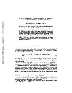
Figure 1. Comparison between the variational approximation and the numerical solution for the lowest order eigen function.

where the coefficients α ; β and γ are given by α = 1=6 + (1=3)(ln 2); β = ln 2, γ = (2=3) ln 2 1=6: The variational equations with respect to A and a determine the eigenvalue, δ , and the width, a, in terms of the amplitude A as follows

δ

=

γ 2 A  0:21A2 2β

r

aA =

2α γ

 1 65 :

;

(16)

in very good agreement with the numerically obtained solution (δ numerical  0:21A2) and figure 1. 5. Stationary vortex solutions of the NLS equation In a number of applications in nonlinear optics, vortex solutions to the two dimensional NLS equation play an important role. Stationary vortex solutions of eq. (10) are of the form ψ (t ; r; θ ) = ρ (r) exp(imθ iδ t ), where m denotes the mode number of the vortex. The corresponding equation for ρ (r) then becomes, [3]



dρ 1 d r r dr dr



m2 ρ r2

δρ + ρ3 = 0

(17)

where ρ ! A as r ! ∞ and ρ ! 0 as r ! 0. However, the boundary condition at infinity directly determines the eigenvalue to be δ = A 2 . We can use this fact to normalize eq. (17) Pramana – J. Phys., Vol. 57, Nos 5 & 6, Nov. & Dec. 2001

921

D Anderson, M Lisak and A Berntson by introducing ρ =A ! ρ ; rA ! r, which is equivalent to setting A = 1 in eq. (17). The Lagrangian corresponding to the stationary vortex equation can then conveniently be taken as L=



1 2

dρ dr

2 +

m2 2 ρ 2r2

1 2 (ρ 4

1)2 :

(18)

As regards a proper choice of trial function, we note that the solution of the vortex equation clearly has the asymptotic dependence ρ  r m as ρ ! 0. A suitable trial function satisfying the asymptotic requirements as r ! 0 and r ! ∞ is ρ = tanh m (ar ). However, when we insert this expression into the Lagrangian, the corresponding integral from zero to infinity is divergent. This problem can easily be circumvented by defining

Z

hLR i =

R 0

L(ρT )r dr:

(19)

For simplicity taking m = 1 we obtain

hLR i = 12

Z

aR

xsech 4 x dx +

0

1 2

Z

aR

0

1 1 tanh2 x dx + a2 x 4

Z

aR

xsech 4 x dx:

(20)

0

The variation of hL R i with respect to the free parameter a yields

∂ hLR i ∂a

= aR

2

1 sech 4 (aR) + tanh2 (aR) a

1 a3

Z

aR

xsech 4 xdx +

0

R2 sech 4 (aR): 2a (21)

The proper reduced variational equation for L is then taken as

∂ hLi ∂a

∂ hLR i  Rlim =0 !∞ ∂ a

(22)

:

All terms in eq. (22) have finite limits as R ! ∞ and we obtain the simple result

Z

a=

∞

xsech 4 xdx

1=2

0

' 0 543 :

:

(23)

A comparison between the numerically obtained solution and the variational approximation is shown in figure 2. The agreement is seen to be very good.

6. Stationary solutions of the NLS equation in graded index optical fibres and BoseEinstein condensates Optical beam propagation in a graded index fibre can be described by the following generic equation, [4] i 922

∂ψ ∂z

2 = ∇? ψ + Vextψ + U

jψ j2ψ

;

Pramana – J. Phys., Vol. 57, Nos 5 & 6, Nov. & Dec. 2001

(24)

Nonlinear evolution equations in optics

1

ρ

0.5

0

0

5

10 r

15

20

Figure 2. Comparison between the variational approximation and the numerical solution for the lowest order vortex solution.

where Vext denotes an external focusing potential ( i.e. signV ext = 1) and the sign of U may be either focusing (sign U = +1) or defocusing (sign U = 1). In the case of a graded index medium, the focusing is caused by the radial variation (for simplicity assumed parabolic) of the refractive index, which decreases outwards in the medium. The nonlinearity in the Kerr medium is also focusing, implying that linear and nonlinear effects are working in the same direction. The corresponding equation describes the transverse dynamics of the slowly varying beam wave envelope as it propagates in the medium (the evolution variable is z) . However, in the case of Bose-Einstein condensates, the external potential is created by a magnetic trap, which also gives rise to a confining potential, usually considered as parabolic in the spatial coordinate. For two dimensional radially symmetric traps, the linear potentials for the two seemingly unconnected physical situations become completely equivalent. On the other hand, in the Bose-Einstein condensates, the nonlinear potential may be either focusing or defocusing depending on whether the ‘scattering length’ of the two body interaction is positive or negative. The only formal difference between the two cases is the evolution variable, which in the case of the Bose-Einstein condensates is time instead of the distance of propagation as in the case of the optical fibre. However, in both cases the characteristic eigenvalue equation for the mode profile can be written in the normalized form



1 d dρ r r dr dr



δρ

r2 ρ  ρ 3 = 0;

where  refers to focusing (+) and defocusing ( corresponding to eq. (25) is L=

1 2



dρ dr

2

+

(25) ) situations respectively.

1 2 1 δ ρ + r2 ρ 2  ρ 4 : 2 4

The Lagrangian

(26)

It is well-known that this solution, in the absence of the nonlinearity has Gaussian shaped solutions. Intuitively we expect that the influence of the nonlinearity is to compress the Pramana – J. Phys., Vol. 57, Nos 5 & 6, Nov. & Dec. 2001

923

D Anderson, M Lisak and A Berntson profile and make it more peaked in the focusing case and to broaden the profile and make it more rectangular in the defocusing case. A suitable trial function, which has the inherent flexibility to model these features is the super Gaussian i.e. we choose as trial function in the variational procedure

ρ (r) = ρT (r) = A exp



1  r 2m 2 a



(27)

:

This trial function involves the previous parameters, width and amplitude, but also an additional new parameter - the super Gaussian index m, which allows for a more flexible ansatz. In particular, it makes it possible to model the change of profile towards a ‘sharper than Gaussian’ profile in the focusing case (m < 1) and a ‘broader than Gaussian’ profile (m > 1) in the defocusing case. The reduced Lagrangian now becomes Z∞ hLi  L(ρT )rdr = I0 A2 + δ I1a2A2 + I2a4A2  I3a2A4 (28) 0

where the coefficients I j , j = 0; 1; 2; 3 are explicit functions of m given by (Γ(x) denotes the gamma function): Z m2 ∞ 4m 1 m I0 = x exp ( x2m )dx = 2 0  4  Z 1 ∞ 1 1 I1 = x exp ( x2m )dx = Γ 1 + 4 0 4 m   Z 1 ∞ 3 1 2 2m I2 = x exp ( x )dx = Γ 1 + 2 0 8 m   Z∞ 1 1 2m (2+1=m) I3 = x exp ( 2x )dx = 2 Γ 1+ (29) : 2 0 m The variational equations with respect to a; A and m are again algebraic equations, which can be rewritten in the following form: A2 a 2 = 

mp(m) I3

a4 =

m[1

p(m)] 2I2

δ

=

m[3p(m) 2] : 2a2 I1

(30)

The characteristic function p(m) is given by p(m) 

m + 2[ψ (1 + 1=m) ψ (1 + 2=m)] ; ln 2 + 2[ψ (1 + 1=m) ψ (1 + 2=m)]

(31)

where ψ (x) denotes the logarithmic derivative of the Gamma function. The form of p(m) is very simple; it varies monotonously from its highest possible physical value ( p = 1) (the self focusing threshold) which is attained for m = ln 2, passes p = 0 for m = 1 (the linear case) and approaches ∞ (the strongly defocusing case) as m approaches mcrit ' 2:5. The part of the curve where p(m) > 0 is relevant for the focusing case whereas the complementary part, where p(m) < 0, is applicable to the defocusing situation. Some examples of the agreement between numerical calculations and the variationally obtained results are shown in figures 3–7. Figures 3–6 refer to the focusing case. In particular, figures 3 and 4 show a comparison between the stationary profiles for two different

924

Pramana – J. Phys., Vol. 57, Nos 5 & 6, Nov. & Dec. 2001

Nonlinear evolution equations in optics 6 variational numerical 5

ρ

2

4

3

2

1

0

0

0.5

1

1.5

2

2.5

r

Figure 3. Comparison between profiles for p = 0:67.

25 variational numerical

20

ρ2

15

10

5

0

0

0.5

1

1.5

r

Figure 4. Comparison between profiles for p = 0:95.

Pramana – J. Phys., Vol. 57, Nos 5 & 6, Nov. & Dec. 2001

925

D Anderson, M Lisak and A Berntson 3 variational numerical

2

µ

1

0

−1

−2

−3

0

1

2

3

4

5

6

7

8

9

10

A2

Figure 5. Comparison between the numerical and approximate results for the eigenvalue.

variational numerical 10

N

8

6

4

2

0

0

5

10

15

20

25

30

35

40

45

50

A4

Figure 6. Comparison between the numerical and approximate results for the total beam power.

926

Pramana – J. Phys., Vol. 57, Nos 5 & 6, Nov. & Dec. 2001

Nonlinear evolution equations in optics 4 variational numerical Thomas−Fermi

3.5

3

ρ2

2.5

2

1.5

1

0.5

0

0

0.5

1

1.5

2

2.5

3

3.5

r

Figure 7. Comparison between profiles for p =

2 in the defocusing case.

values of p in the self focusing regime and figures 5 and 6 compare the corresponding predictions for the eigenvalue δ and the total power (or equivalently the total number of condensates). Finally, figure 7 compares the numerically obtained mode profile in the case of defocusing nonlinearity with the variational approximation and the Thomas-Fermi approximate solution, obtained by simply balancing the focusing of the external trap with the defocusing due to the nonlinearity i.e. ρ 2 ' µ r2 . The approximate analytical approaches yield very similar results for the eigenvalue and the total number of particles. In the limit of large nonlinearity, when the Thomas-Fermi approximation is known to be a good approximation, we have for the eigenvalue µ , µ T F = α A2 where αT F = 1 and αV = (1=2)I32 (mcrit )=I2 (mcrit ) ' 1:14 For the total number of particles, N, we have N = β A 4 where βT F = 1=4 and βV = (3=2)I3(mcrit )=I1 (mcrit ) ' 0:243. 7. Solutions of the Pereira-Stenflo equation Although most generalizations of the NLS equation do not allow explicit exact solutions, some classical examples of the opposite situation do exist. As an example we consider the so-called Pereira-Stenflo equation, [5], a generalization of the classical NLS equation, where the coefficients of the dispersive and nonlinear terms are allowed to be complex and also linear growth is included. The physical basis for this generalization are dispersive wave filtering and nonlinear damping. In the case of anomalous dispersion the normalized Pereira-Stenflo equation can be taken as, [5]

Pramana – J. Phys., Vol. 57, Nos 5 & 6, Nov. & Dec. 2001

927

D Anderson, M Lisak and A Berntson i(1

γ0 )

∂ ψ + (1 ∂t

iγ2)

∂ 2ψ ∂ x2

jψ j2 ψ = 0

+ (1 + iγn )

(32)

:

For variational purposes we note that this equation can be rewritten as

δ L0 δ ψ

= iR[ψ ]

(33)

where L0 is the Lagrangian corresponding to the basic NLS part and the operator R[ψ ] accounts for the additional terms i.e.,

δ L0 δ ψ

=i

∂ψ ∂t

∂ 2ψ ∂ x2

+

+

jψ j2ψ

R[ψ ] = γ0 ψ + γ2

∂ 2ψ ∂ x2

γn jψ j2 ψ :

(34)

In this case, the variational equations for the parameter functions, p j (t ), become

δ L0 δ pj

Z = 2Re

+∞

∞

iR[ψs ]

∂ ψs dx: ∂ pj

(35)

Guided by the properties of the classical soliton and the form of the stationary solution found by Pereira and Stenflo, we use a trial function of the following form

ψs (t ; x) = A(t )sech [B(t )x] exp[iφ (t ) + iα (t ) ln sech B(t )x]:

(36)

For simplicity we restrict the analysis to the stationary case. The parameters A; B and α are then constants and φ (t ) is of the form φ (t ) = δ t. The corresponding reduced basic Lagrangian is given by 2 hL0 i = 2 AB



dφ dt

1 2 1 B (1 + α 2 ) + A 2 3 3

 :

The variational equations with respect to the parameters become (z = Bx) Z +∞ Re sech z exp( iθ )R[ψT ]dz = 0 ∞ Z +∞ 2 α AB2 = Re sech z ln sech z exp( iθ )R[ψT ]dz 3 ∞ Z +∞ 2 2 4 3 2 A = Im sech z exp( iθ )R[ψT ]dz 2δ A + AB (1 + α ) 3 3 ∞ Z +∞ 1 2 1 3 AB (1 + α 2 ) A = Im δA sech z exp( iθ ) tanhzR[ψT ]dz 3 3 ∞ Z +∞ α Re sech z exp( iθ ) tanhzR[ψT ]dz; ∞

(37)

(38)

where θ = δ t + α ln sech z. Inserting the form of R[ψ ] specific for the Pereira–Stenflo equation, the parameters of the stationary solution become completely determined by the coefficients as follows:

928

Pramana – J. Phys., Vol. 57, Nos 5 & 6, Nov. & Dec. 2001

Nonlinear evolution equations in optics

 A

2

= 2B

3 1 + αγ2 2

2

α

β+

=

p

1 2 α 2

 B2 =

β2 +2

δ

γ2 2α + γ2 (α 2

= B (1 + 2αγ2 2

1)

α 2)

(39)

where the parameter β is given by

β

=

3 1 γ2γn : 2 γ2 + γn

(40)

The stationary equation found by the variational procedure is identical to the exact stationary soliton solution obtained by Pereira and Stenflo, as indeed it should since the exact solution is contained within the set of trial functions.

8. Dynamical evolution of non-soliton intial conditions for the NLS equation In the present section we will discuss the dynamical evolution of initially sech-shaped pulses with initial conditions, which do not correspond to stationary conditions for the NLS equation. More specifically we will consider the normalized NLS equation in the standard form: i

∂ψ ∂t

+

1 ∂ 2ψ 2 ∂ x2

jψ j2ψ = 0

(41)

together with the initial condition ψ (0; x) = A 0 sechx exp(ib0 x2 ). The signs + and - correspond to the cases of anomalous and normal dispersion respectively. In the case of anomalous dispersion and for A 0 = 1 and b0 = 0, the corresponding solution is the one-soliton solution ψ S (t ; x) = sech x exp(it =2). In the case A 0 < 3=2, the solution exhibits an initial dynamical stage involving oscillations of amplitude and width and eventually the pulse separates into a decaying dispersive radiation part and an asymptotic stationary soliton solution of the form ψ S (t ; x) = η sech (η x) exp(iη 2t =2) where the asymptotic soliton amplitude η according to inverse scattering theory is given by η = 2A 0 1 when b0 = 0. A complete treatment of the oscillatory stage can only be obtained numerically. However, significant information can also be obtained using the variational approach, [6]. A suitable trial function, flexible enough to incorporate the main dynamical features of the solution and compatible with the initial conditions can be taken as





x ψT (t ; x) = A(t )sech exp[ib(t )x2 + iφ (t )] a(t )

(42)

:

This choice of trial function is also based on physical intuition derived from known properties of linear dispersive as well as nonlinear self phase modulated pulse dynamics. With this ansatz the reduced Lagrangian becomes

hLi =

 aA2 2

dφ dt

+

π 2 2 db a 6 dt



1 2 A 3



1 2 3 2 +π a b a



 23 aA4

Pramana – J. Phys., Vol. 57, Nos 5 & 6, Nov. & Dec. 2001

:

(43)

929

D Anderson, M Lisak and A Berntson The variational equations with respect to A; a; b and φ can, after some rearrangement, be written as three explicit expressions for b(t ); A(t ) and φ in terms of the pulse width, a(t ) viz., b(t ) =

1 d ln a(t ) 2 dt

A2 =

dφ dt

A20 a

1 5 A20  2 3a 6 a

=

(44)

and the pulse width is determined by a single second order autonomous differential equation, which directly can be integrated once to yield the suggestive potential function description 1 2



da dx

2

+ Π(a) = W

4A20 1 2 1  π 2 a2 π2 a  2 4A20 1 da 2 2 (0) + Π(a(0)) = 2b 0  : 2 dx π2 π2 Π(a) =

W

=

(45)

This equation has the form of a unit mass particle moving in a nonlinear potential field given by Π(a) and the qualitative dynamical properties of the evolution of the pulse can easily be inferred from the properties of the potential, cf. [1], to give the stability of stationary solutions, nonlinear pulse compression and decompression (depending on the relative signs of dispersion and nonlinearity) and also features like the soliton content of the original pulse.

9. Beam dynamics in a parabolic index medium The variational approach can also be used to obtain important information about the dynamical properties of the beam evolution in a graded index optical medium/cylindrical trapped Bose–Einstein condensate, cf eq. (25). Ideally, the trial function should include the possibility to model the dynamically varying radial shape function of the beam e.g. by using a super Gaussian trial function with a super Gaussian index, m that varies with distance of propagation i.e. m = m(z). However, the corresponding variational algebra becomes prohibitively complicated and as a compromise between flexibility and simplicity, the trial function can be chosen as [7]

ψT (z; r) = A(z) exp



r2 2a(z)2



+ ib(z)r + iφ (z) 2

:

(46)

If the dynamic equation is taken in the form i

∂ψ ∂z

=

1 ∂ ∂ψ r r ∂r ∂r

+r

2

ψ jψ j2 ψ ;

(47)

the variational equations for the reduced Lagrangian can be rearranged to give A(z), b(z) and φ (z) in terms of a(z), viz.

930

Pramana – J. Phys., Vol. 57, Nos 5 & 6, Nov. & Dec. 2001

Nonlinear evolution equations in optics a(z)A(z) = constant = a(0)A(0) 1 d lna(z) b(z) = 4 dz   dφ 2 3p = 1  : dz a2 (z) 2

(48)

The characteristic parameter, p is given by p = a 2 (0)A2 (0)=4  A2 (0)=A2c where Ac = 2=a(0) is the critical threshold amplitude at which self-focusing balances diffraction. The beam width parameter a(z) satisfies the the same type of potential equation as in the previous section, but the potential is now given by 1 2 Π(a) = a2 + 2 ( p 2 a

1):

(49)

This equation provides a simple starting point for an analysis of the properties of the self focusing dynamics of a laser beam (or a Bose–Einstein condensate) in a parabolic external potential.

10. Dispersion-managed solitons Dispersion-management is an attractive way to increase the capacity of optical communication systems. By composing a fibre link of fibres with opposite sign of the chromatic dispersion, the path-average dispersion can be kept low so that penalties due to dispersion are small. This technique is commonly used today in commercial communication systems together with the non-return-to-zero (NRZ) modulation format [8]. In 1995 it was shown that dispersion-management also can improve the performance of soliton systems [9]. There are pulses, so-called dispersion-managed solitons, which in a periodic dispersion-management reproduce themselves with the period of the dispersion map, one example is shown in figure 8, see also [14] . The long-scale (from one dispersion period to the next) dispersive pulse broadening is stopped due to a balance between dispersion and nonlinear effects. Notice in figure 8 the large variation of the spectral width of the pulse, and the pulse parameters evolving periodically in spite of a non-zero path-average dispersion, both these effects are manifestations of the fibre nonlinearity. The advantages of dispersion-managed solitons compared with solitons in fibres with uniform dispersion include enhanced energy [11], leading to reduced Gordon-Haus jitter [12], and reduced pulse interaction [13]. The variational approach is the ideal tool for studying this problem, since the large number of parameters involved (two fibres with different properties and lengths) makes a full numerical study cumbersome. The variational approach has captured the essence of dispersion-managed solitons, (eg the power enhancement and the pulse dynamics [15,16,14]) with good accuracy . Here we will discuss two-stage maps where the dispersion alternates between positive (normal) and negative (anomalous) following [14]. The pulse evolution is modeled by the nonlinear Schr¨odinger equation, which with standard notations for optical fibres is written iuz

=

β 00 uττ 2

γ juj2u

Pramana – J. Phys., Vol. 57, Nos 5 & 6, Nov. & Dec. 2001

(50) 931

Spec width, GHz

D Anderson, M Lisak and A Berntson

30

25

20

Pulse width, ps

70 60 50 40 30

D, ps/(nm*km)

20

16

0

−16 0

50

100

150

200

Distance of propagation, km

Figure 8. Example of evolution of the pulse width and the spectral width of a dispersion-managed soliton.

where z is the distance of propagation, t is the time in the group velocity frame, γ and β 00 are the nonlinear coefficient and the dispersion of the fibre respectively. Normalizing p eq. (50) according to τ = t =Tc , U = u= Pc , where Tc is a characteristic time and Pc a characteristic power, we obtain iUζ

=

sgn(β 00 ) Uττ 2

γ Pc Tc2 2 jβ 00j jU j U

(51)

where ζ is the distance of propagation measured in dispersive lengths, L D = Tc2 =jβ 00 j. Equation (51) has just one parameter, the coefficent in front of the nonlinear term given by γ =β 00 . A two-stage dispersion map is defined by four parameters, the ratio γ =β 00 in each of the two fibres and the lengths of the two fibres. By requiring self-replication after one dispersion period, the number of parameters is reduced to three, e.g. with γ =β 00 given in both fibres, the lengths are no longer independent. We will use the map 2 strength S = j(β100 L1 β200L2 )j=τFWHM [13,16,17,14] as the single quantity describing the fibre lengths. As a measure of the power we introduce the normalized peak power, 2 00 00 refer to the anomalous dispersion fibre, P is N 2 = γ P0 τFWHM =(3:11jβ j), where γ and β 0 the peak power and τ FW HM is the full width at half maximum (FWHM), both taken at the midpoint of the anomalous fibre. The normalized power gives the pulse peak power, at the mid-point of the anomalous dispersion fibre in fractions of the power of the fundamental soliton of the same FWHM. We will now obtain approximate solutions to eq. (51) by means of the variational approach. For this purpose we use the Gaussian ansatz function 932

Pramana – J. Phys., Vol. 57, Nos 5 & 6, Nov. & Dec. 2001

Nonlinear evolution equations in optics

 u = A(z) exp



τ 2 (1 ib(z)) + iΦ(z) 2a(z)2

(52)

with a yet unspecified dependence of the parameter functions A, a, b and Φ, on z. The ansats, eq. (52), is inserted into eq. (8) with the Lagrangian given by eq. (11) and R = 0. The Euler–Lagrange equations of the reduced problem is a set of four coupled ordinary differential equations for the parameter functions. This system can be reduced to yield a single second order differential equation for the normalized pulse width, y(ζ ) = a(ζ )=a(0), d2 y dζ 2

=

1 y3

+

2 NVA p y12 2

(53)

2 = γ A(0)2 a(0)2 =β 00 . where ζ is the distance along the fibre in L D = a(0)2 =jβ 00 j and NVA 0 The chirp, b, is given by b = yy ζ . Equation (53) can be solved analytically [1] to give

z = f (y(z))

f (y) =

1 C

f (1)

q

Cy2

(54)



2 y 2NVA

1+

2 NVA p ln y C

2 NVA C

+

q

Cy2

 2 y 2NVA

1 (55)

2 + 1 is a constant. Starting with a chirped pulse between the where C = y0ζ (0)2 + 2NVA 2 in both fibres, eq. (55) fibres in a dispersion map, i.e., with given b(0), and with given N VA can be used to calculate the distance after which the pulse is unchirped and the minimum pulse width in both the anomalous and the normal dispersion fibre. From this the average dispersion follows, and also N 2 and S. Using this method we can build up a dependence on the peak power and map strengths for solitons with various normalized average dispersions, figure 9a. The figure is a contour plot, for the case of two equally nonlinear fibres (equal γ =jβ 00 j), each line corresponding to 00 =β 00 (β 00 is the dispersion of the anomalous fixed normalized average dispersion, β¯ 00 = βave dispersion fibre) in the map strength / power plane. We stress that the system is in this case (equally nonlinear fibres) completely determined by N 2 and S, and that the normalized 2 fibre lengths (β n Ln =τFWHM ) can be calculated from this without further assumptions. A fixed dispersion map (fixed β 1 ; L1 ; β2 and L2 ) corresponds to a line of constant β¯ 00 and the variation in S and N 2 along this line is achieved by varying the pulse width and peak power. When constructing a line with constant β¯ 00 = βC we first have to make an assumption of 2 at the fibre boundary and from this calculate β¯ 00 . In general the result will be b(0) and NVA different from βC and we have to make a new guess, e.g. with a different b(0). When we have found the proper b(0) we have a point on the line β¯ 00 = βC . Next we pick a new guess 2 at the fibre boundary and the procedure is repeated to find the corresponding b(0) of NVA which gives a second point along the line in figure 9a. The predictions of the variational approach were qualitatively verified by a numerical investigation, shown in figure 9b. Each point in figure 9b corresponds to a numerical solution of the full NLS-equation, found using the method in [17]. For high powers or for strong maps the pulses radiate, which limits the range of solutions in figure 1b to approximately N 2 < 0:6 and S < 12. Several important properties of dispersion-managed solitons are demonstrated by figure 9. Firstly, above a critical strength of S = 3:9 (S = 4:8 variationally) there is a region

Pramana – J. Phys., Vol. 57, Nos 5 & 6, Nov. & Dec. 2001

933

D Anderson, M Lisak and A Berntson 1

(a)

0.9

Higher order solutions Normalised peak power

0.8 0.7

Anomalous net dispersion

0.6 0.5

Normal net dispersion

0.4 0.3 0.2 0.1 0 0

2

4

6

8

10

12

14

16

18

20

Map strength, S 1

(b) 0.9

Normalised peak power

0.8 0.7 0.6 0.5 0.4 0.3 0.2 0.1 0 0

2

4

6

8

10

12

14

16

18

20

Map strength, S

Figure 9. Contour plot of β¯ 00 as function of map strength and peak power. In (a) the variational result with lines for β¯ 00 = 0.01, 0.05, 0.1, 0.2, 0.3 and 0.5 (anomalous average dispersion, solid lines), β¯ 00 = 0 (bold line), and for β¯ 00 = 0.001, 0.005, 0.01, 0.02 (normal average dispersion, dashed lines). The dotted line represents an example of constant energy. In (b) results from numerical solutions of the full NLS-equation. Each point represents a calculated stationary solution, the lines drawn between the points join sets of solutions for the same β¯ 00 , shown in the figure are β¯ 00 = 0:2; 0:1; 0:01, β¯ 00 = 0 and β¯ 00 = 0:01; 0:02.

934

Pramana – J. Phys., Vol. 57, Nos 5 & 6, Nov. & Dec. 2001

Nonlinear evolution equations in optics 0.7

Lines corresponding to S = 0, 2, 4, ... 20, and 25

Normalised peak power

0.6

0.5

0.4

0.3

0.2

0.1

0 −0.2

Normal

Anomalous

dispersion

dispersion 0

0.2

Normalised average dispersion

Figure 10. Normalized peak power as function of β¯ 00 . for constant map strengths, from right to left the lines correspond to S = 0; 2; 4; 6; 8; :::; 20, and 25.

which allows stable propagation at zero and normal average dispersion. A general property is that as the map strength is increased (for constant power or energy) the average dispersion is shifted towards normal dispersion. Secondly, the variational approach predicts two solutions for the same energy in the normal average dispersion regime. This can be seen from the dotted line in figure 9a representing constant energy. Only the upper branch of the possible solutions was found numerically, suggesting that the lower branch represents unstable solutions. This means that there is a power threshold for the existence of stable pulses in the normal dispersion regime. The threshold value depends on the average dispersion and in the linear limit ( β¯ 00 ! 0) it goes to zero. Note that the dividing point between the stable and the unstable branch occurs for minimum energy and not for minimum map strength. As a consequence of this, for a fixed dispersion map ( β¯ 00 = constant) there can be two solutions with different powers for the same pulse width. The region marked ‘higher order solutions’ in figure 9a represents a situation with soliton formation where the anomalous fibre is longer than a soliton period. This region is excluded from figure 9a partly for the sake of clarity and also because the same solution can always be achieved by a shorter anomalous fibre period i.e. with a lower average dispersion (by removing a piece corresponding to a soliton period). Figure 10 shows the variational result for the normalized power as function of the normalized average dispersion. If the strength is larger than 4.8 the lines for constant S penetrate into the normal dispersion and reach a maximum normal dispersion. Note that 00 = 0 is not a special case, for S > 4:8 there is a smooth change-over from anomalous βave to normal average dispersion as indicated by figure 2.

Pramana – J. Phys., Vol. 57, Nos 5 & 6, Nov. & Dec. 2001

935

D Anderson, M Lisak and A Berntson 11. Summary The present work has reviewed the main ideas behind the variational approach and has given some illustrative examples of its use in present day nonlinear optics. The main advantage of the approach is that it gives simple and explicit (albeit approximate) expressions for physically relevant quantities in situations where exact analytical solutions are not available or may be too complicated to provide the necessary physical insight and also in situations where only numerical solutions can be found. The method is flexible and can easily be adopted to apply to different, both stationary and dynamical, problems in a variety of situations. A drawback of the method is that it is based on the use of trial functions. In order to have an accurate approximation of the solution, a good choice of trial functions must be made. However, this requires some prior knowledge of the expected physical behaviour of the system under study. Such knowledge is usually obtained either by physical intuition or by numerical simulations. Another drawback is that it is difficult to determine a priori the accuracy of the obtained approximate solution. This implies that the results have to be checked, at least for some typical parameters, against numerically obtained results.

References [1] D Anderson, Phys. Rev. A27, 3135 (1983) [2] D Anderson, M Bonnedal and M Lisak, Phys. Fluids 22,1838 (1979) [3] A H Carlsson, J N Malmberg, D Anderson, M Lisak, E A Ostrovskaya, T J Alexander and Yu Kivshar, Optics Lett. 25, 660 (2000) [4] M Karlsson and D Anderson, J. Opt. Soc. Am. B9, 1558 (1992) [5] D Anderson, F Cattani and M Lisak, Physica Scr. T82, 32 (1999) [6] D Anderson, M Lisak and T Reichel, J. Opt. Soc. Am. B5, 207 (1988) [7] M Karlsson, D Anderson, M Desaix and M Lisak, Optics Lett. 16, 1373 (1991) [8] G P Agrawal, Fiber-optic communication systems (Wiley & Sons, New York, 1997) [9] M Suzuki, I Morioka, N Edagawa, S Yamamoto, H Taga and S Akiba, Electron. Lett. 31, 2027 (1995) [10] J H B Nijhof, N J Doran and W Forysiak, Opt. Lett. 23, 1674 (1998) [11] N J Smith, N J Doran, F M Knox and W Forysiak, Opt. Lett. 21, 1981 (1996) [12] A Hasegawa, Y Kodama and A Maruta, Opt. Fibre Tech. 3, 197 (1997) [13] T Yu, E A Golovchenko, A N Pilipetskii and C R Menyuk, Opt. Lett. 22, 793 (1997) [14] A Berntson, N J Doran, W Forysiak and J H B Nijhof, Opt. Lett. 23 , 900 (1998) [15] I Gabitov, E G Shapiro and S K Turitsyn, Opt. Commun. 134, 317 (1997) [16] V S Grigoryan, T Yu, E A Golovchenko, C R Menyuk and A N Pilipetskii, Opt. Lett. 22, 1609 (1997) [17] J H B Nijhof, N J Doran, W Forysiak and F M Knox, Electron. Lett. 33, 1726 (1997)

936

Pramana – J. Phys., Vol. 57, Nos 5 & 6, Nov. & Dec. 2001