A Variational Approach to Semi-Supervised Clustering

A Variational Approach to Semi-Supervised Clustering Peng Li, Yiming Ying and Colin Campbell Department of Engineering Mathematics, University of Bristol, Bristol BS8 1TR, United Kingdom Abstract. We present a Bayesian variational inference scheme for semisupervised clustering in which data is supplemented with side information in the form of common labels. There is no mutual exclusion of classes assumption and samples are represented as a combinatorial mixture over multiple clusters. We illustrate performance on six datasets and find a positive comparison against constrained K-means clustering.

1

Introduction

With semi-supervised clustering the aim is to find clusters or meaningful partitions of the data, aided by the use of side information. This side information can be in the form of must-links (two samples must be in the same cluster) and cannot-links (two samples must not belong to the same cluster). A number of approaches have been proposed for semi-supervised clustering including modifications of pre-existing clustering schemes such as incremental clustering algorithms [1] or K-means clustering [2]. One problem with some of these approaches is that the method can work well if the correct number of clusters is already known: K-means clustering is an example. However, a principled approach to finding K is generally not given. Other potential disadvantages of some clustering approaches is that there is an implicit mutual exclusion of clusters assumption. In many applications this assumption may not be fully valid and it would be more appropriate for a sample to be associated with several clusters. Our motivation for considering semi-supervised clustering comes from potential applications in cancer informatics. There have been a number of instances where unsupervised learning methods have been applied to cancer expression array datasets and clinically distinct cancer subtypes have been indicated e.g. [3, 4]. However, in some cases a specific causative event is known and thus it is possible to give common labels to some samples. In these cancer applications, the side information is typically in the form of must-links: these will be the focus of this paper. We thus propose a probabilistic graphical model approach to semi-supervised clustering with samples represented as combinatorial mixtures over a set of soft clusters. By allowing a representation overlapping different clusters we can derive a confidence measure for cluster membership. In clinical cancer applications, a subtype assignment confidence measure is plainly important. In the next section we propose our probabilistic graphical model, followed by experiments in section 3.

2

The Method

Our semi-supervised model utilizes the Latent Process Decomposition (LPD) model developed in [5, 6], and hence we will call this variant semi-supervised LPD or SLPD. For the natural numbers we adopt the notation Nm = {1, . . . , m} for any m ∈ N. For the data we use d as the sample index, g as the attribute index, and script letters D, G to index the corresponding number of samples and attributes. The number of clusters is K. The complete data set is E = {Edg : d ∈ ND , g ∈ NG }. This notation stems from our cancer informatics motivation of expression value of gene g in sample d. In our semi-supervised setting, we have additional block information C where each block c denotes a set of data points that is known to belong to a single class. In keeping with standard Bayesian models, we also assume both blocks and the data points in each block are i.i.d. sampled. Specifically, this side information can be represented by a D × C matrix δ with its entities δdc defined as follows ½ 1 if data d is a member of block c, δdc = 0 otherwise. In probabilistic terms, the dataset E will be partitioned into K soft clusters described as follows. For a complete data set, a Dirichlet prior distribution for the distribution of clusters is defined by a K-dimensional parameter α. For each known block c, a distribution θc over the set of mixture components indexed by k is drawn from a single Dirichlet distribution parameterized by α. Then, for all samples d in block c (i.e. δdc = 1), the latent indicator variable Zdg indicates which cluster k is chosen, with probability θck , from the common block-specific distribution θc . The value Edg for attribute g in sample d is then drawn from the kth Gaussian with mean µgk and deviation σgk , denoted as N (Edg |µgk , σgk ). We repeat the above procedure for each block in C. The graphical model is illustrated in Figure 1 which is motivated by Latent Dirichlet Allocation [5]. The model parameters are Θ = (µ, σ, α) and we use the notation d ∼ c to denote sample d in block c. From the graphical model in Figure 1, we can formulate the block-specific joint distribution of the observed data E and the latent variables Z by Y Y p(E, θ, Z|Θ, C) = p(θc |α) p(Ed , Z|θc , Θ), (1) c

d∼c

where p(θc |α) is Dirichlet defined by p(θc |α) = block matrix δ, we further see that Y

p(Ed , Z|θc , Θ)

=

P

k

k αk ) Γ(αk )

Q k

αk −1 θck . Using the

· ¸δdc p(Z |θ )p(E |Z , µ, σ) d c d d d

Q

d∼c

=

Γ( Q

Q Q d

g

·

¸δdc p(Zdg |θc )N (Edg |µg , σg , Zdg ) .

(2)

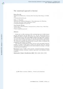
Fig. 1: A graphical model representation of the method proposed in this paper. Edg denotes the value of attribute g in sample d. µ and σ are model parameters. Zdg is a hidden variable giving the cluster index of attribute g in sample d. θc gives the mixing over subgroups for sample d in block c denoted by d ∼ c. The probability of θc is given by a Dirichlet distribution with hyper-parameter α. For notational simplicity, we regard Zdg as a unit-basis vector (Zdg,1 , . . . , Zdg,K ) which transforms the cluster latent variable Zdg = k to the unique vector Zdg given by Zdg,k = 1 and Zdg,j = 0 for j 6= k. Equivalently, the random variable Zdg is distributed according to a multinomial probability defined by Q Z p(Zdg |θc ) = k θckdg,k . Hence, the above equation can be rewritten as

p(E, θ, Z|Θ, C) =

Y

p(θc |α)

c

Y Y Y· d

g

¸Zdg,k δdc θck N (Edg |µgk , σgk ) .

(3)

k

With these priors, the final data likelihood can be obtained by marginalizing out the latent variables θ and Z := {Zdg : d ∈ ND , g ∈ NG } Z X p(E, θ, Z|Θ, C)dθ. (4) p(E|Θ, C) := θ Z

In particular, we can see from equations (2) and (3) that ¸δdc Y Z X Y Y· p(E|Θ, C) = p(Zdg |θc )N (Edg |µg , σg , Zdg ) p(θc |α)dθc = =

YZ

θc Z

c

g

d ¸Zdg,k Y · θck N (Edg |µgk , σgk ) p(θc |α)dθc

X

c

θc Z ,d∼c d∼c,g,k dg

c

θc d,g

Y Z Y·X

¸δdc θck N (Edg |µg , σg , Zdg ) p(θc |α)dθc .

k

(5) We should mention that, without block information (i.e. δ = ID×D ), the above equation is the exact likelihood of Latent Process Decomposition given in [6]. We now consider model inference and parameter estimation under SLPD. The main inferential goal is to compute the posterior distribution of the hidden variables p(θ, Z|E, Θ, C). One direct method is to use Bayes rule p(θ, Z|E, Θ, C) =

p(E,θ,Z|Θ,C) p(E|Θ,C) .

This approach is usually intractable since this involves computationally intensive estimation of multi-integrals in the final likelihood p(E|θ, C). In this paper, we rely on variational inference methods [7] which maximize a lower bound on the likelihood p(E|Θ, C) to estimate the model parameters Θ and approximate p(θ, Z|E, Θ, C) in a hypothesis family. One common hypothesis family is the factorized family defined by q(θ, Z|γ, Q) = q(θ|γ)q(Z|Q) with variational parameters γ, Q where, in the expression of the distribution q, the dependency on the E, Θ, C is omitted.P More specifically, in our model Q Q ¡ Γ( k γck ) Q γck −1 ¢ we assume that q(θ|γ) = c q(θc |γc ) = c Q Γ(γ , and q(Z|Q) = k θck ck ) k Q Q ¡Q Zdg,k ¢ d,g q(Zdg |Qdg ) = d,g k Qdg,k , among which γ, Q will be set as we describe below. We can lower bound the log-likelihood by applying Jensen’s inequality to equation (4): Z X p(E, θ, Z|Θ, C)dθ log p(E|Θ, C) = log θ Z £ ¤ £ ¤ ≥ L(γ, Q; Θ) := Eq log p(E, θ, Z|Θ, C) − Eq q(θ, Z|γ, Q) . Consequently we can estimate the variational and model parameters by alternative coordinate ascent methods known as a variational EM algorithm: • E-step: maximize L with respect to the variational parameters γ, Q to give the following updates (Ψ(x) is the digamma function): ¤ £Q P N (Edg |µgk , σgk ) c exp(δdc (Ψ(γck ) − Ψ( k γck ))) ¤, £ P Q Qdg,k = P (6) k γck )) k N (Edg |µgk , σgk ) c exp(δdc Ψ(γck ) − Ψ( and γck = αk +

X

δdc Qdg,k

(7)

d,g

• M-step: maximize L with respect to µ, σ and α to give: P P Qdg,k Edg Qdg,k (Edg − µgk )2 2 d µgk = P , σgk = d P . d Qdg,k d Qdg,k

(8)

with the parameter α found using an additional Newton-Raphson method (see Appendix A in [5] for details). The above iterative procedure is run until convergence (plateauing of the lower bound on an estimated likelihood p(E|Θ, C), see [6]). Interpretation of the resultant model is very similar to Latent Process Decomposition [6]. When normalized over k, the parameter γck gives the confidence that a sample belonging to block c (which share a common label) belongs to soft cluster k. For each soft cluster k the model parameters µgk and σgk give a density distribution for the attribute value g over all samples, see [8] for examples of use of these density estimators in application to interpreting breast cancer array data. If some values

Data

UKM

Sets

0

25%

CKM

Letter

0.501±0.005

0.502±0.010

Wine

0.877±0.052

Iris

0.824±0.036

Digit

0.751±0.068

ULPD 50%

SLPD

0

25%

50%

0.501±0.009

0.519±0.025

0.521±0.031

0.527±0.039

0.885±0.051

0.893±0.047

0.930±0.032

0.926±0.032

0.935±0.032

0.825±0.035

0.828±0.041

0.872±0.037

0.910±0.043

0.920±0.038

0.758±0.069

0.772±0.078

0.736±0.046

0.747±0.045

0.755±0.045

Table 1: A comparison of constrained K-means clustering and SLPD. The entries are BRI (over the 100 trials using 3-fold cross validation). Hypothesis testing indicates a statistically significant performance gain over CKM. The highest BRI score per dataset is given in boldtype.

Data Sets Leukemia Lung Cancer

UKM 0 0.786±0.065 0.578±0.030

CKM 25% 50% 0.782±0.061 0.798±0.062 0.583±0.033 0.599±0.041

ULPD 0 0.838±0.053 0.660±0.033

SLPD 25% 50% 0.846±0.049 0.851±0.048 0.665±0.032 0.670±0.039

Table 2: A comparison of constrained K-means clustering and SLPD. The entries are the BRI (mean ± standard deviation over the 50 trials using 3-fold cross validation). Hypothesis testing indicates a statistically significant performance gain over CKM.

of Edg are missing, we omit corresponding contributions in the M -step updates and the corresponding Qdg,k . The above argument is based on a maximum likelihood approach. However, following our original argument [6], we can readily formulate a maximum a posterior (MAP) solution penalising over-complex models which fit to noise in the data and we can perform model selection (to find the number of clusters) using hold-out data [8].

3

Experimental Results

To validate the proposed approach, we investigated the ML solution applied to four datasets from the UCI Repository [9] and two cancer expression array datasets. The four data sets from the UCI Repository have known sample labels and thus we can evaluate an objective performance measure. As mentioned, our interest in semi-supervised clustering stems from a potential use in cancer informatics. Thus we consider two datasets for cancer: leukemia array data [3] in which some labels are known due to causative genetic translocations or rearrangements such as the gene fusion events BCR-ABL or E2A-PBX1. The second dataset is for lung cancer [4]. We investigated three issues. Firstly, a comparison against pre-existing semi-supervised clustering methods, specifically constrained K-means clustering (CKM)[2], since this method is widely used. Secondly, we considered the gains to be made as available label information increases. Finally, we compared unsupervised ULPD with SLPD to evaluate the gains made by using side information. We use the Balanced Rand Index (BRI) as evaluation criterion [10].

In Table 1 we tabulate performance for both constrained K-means clustering and SLPD using BRI with 3-fold random partitioning (one fold being test data, the rest training). Exactly the same sample allocations were used in the evaluation of both constrained K-means clustering and SLPD. For the training set we also imposed a degree of supervision to compare unsupervised learning with semi-supervised clustering using different levels of supervision. The fraction of the supervised data was 0% (unsupervised), 25% and 50%. As observed from Tables 1 and 2, SLPD compares favorably with CKM. With enforcement of a degree of supervision (from 0% to 50%), performance improvement of both SLPD and CKM over LPD and unconstrained K-means clustering (U KM ) is observed. As a real-life application we tested SLPD on two cancer expression array datasets for leukemia and lung cancer (Table 2). For leukemia we find that the BRI index improves as we increase the extent of supervision. We also find that SLPD consistently outperforms K-means clustering. A similar picture is repeated for lung cancer.

References [1] K. Wagstaff and C. Cardie. Clustering with instance-level constraints. In Proceedings of the Seventeenth International Conference on Machine Learning, pages 1103–1110, 2000. [2] S. Basu, A. Banerjee, and R. J. Mooney. Semi-supervised clustering by seeding. In Proceedings of International Conference on Machine Learning 2002, pages 27–34, 2002. [3] E-J Yeoh et al. Classification, subtype discovery, and prediction of outcome in pediatric acute lymphoblastic leukemia by gene expression profiling. Cancer Cell, 1:133–143, 2002. [4] A Bhattacharjee et al. Classification of human lung carcinomas by mRNA expression profiling reveals distinct adenocarcinoma subclasses. Proceedings of the National Academy of Sciences, 98:13790–13795, 2001. [5] D. M. Blei, Andrew Y.Ng, and M. I. Jordan. Latent dirichlet allocation. Journal of Machine Learning Research, 3:993–1022, 2003. [6] S. Rogers, M. Girolami, C. Campbell, and R. Breitling. The latent process decomposition of cDNA microarray datasets. IEEE/ACM Transactions on Computational Biology and Bioinformatics, 2:143–156, 2005. [7] M. I. Jordan, Z. Ghahramani, T. Jaakkola, and L. K. Saul. An introduction to variational methods for graphical models. Machine Learning, 37:183–233, 1999. [8] L. Carrivick, S. Rogers, J. Clark, C. Campbell, M. Girolami, and C. Cooper. Identification of prognostic signatures in breast cancer microarray data using bayesian techniques. Journal of the Royal Society: Interface, 3:367–381, 2006. [9] C.L. Blake D.J. Newman, S. Hettich and C.J. Merz. UCI repository of machine learning databases, http://www.ics.uci.edu/∼mlearn/mlrepository.html, 1998. [10] E. Xing, A. Ng, M. Jordan, and S. Russell. Distance metric learning, with application to clustering with side-information. In Advances in NIPS, number vol. 15, 2003.