A Verification Method for Solutions of Linear Programming Problems PARA’04
Ismail Idriss
Wolfgang V. Walter
[email protected]
[email protected]
University of Applied Sciences/FH Konstanz
Technical University Dresden
June 22, 2004
2
Outline • Basics and Motivation – Problem statement – Motivation and goals – Interior-point methods • Verified Linear Programming – Primal-dual logarithmic barrier method – Mehrotra’s predictor-corrector method – A verification method – Algorithm • Numerical results PARA’04, June 22, 2004
I. Idriss & W. V. Walter, Germany
3
The Linear Programming Problem (LP) Primal Form:
c>x
Minimize
subject to Ax = b
[P]
x≥0 (m equalities, n variables) Dual Form:
Maximize
b> y
subject to A>y + z = c
[D]
z≥0
PARA’04, June 22, 2004
I. Idriss & W. V. Walter, Germany
4
Interior-Point Methods (IPM) Idea: Solve LP via sequence of smooth nonlinear unconstrained optimization problems Fundamental Components of IPM • Logarithmic barrier method to deal with a constrained optimization problem with inequality constraints • Lagrangian function to transform a constrained optimization problem with equality constraints into an equivalent unconstrained problem • Newton’s method to solve unconstrained minimization problem by finding a zero of the gradient
PARA’04, June 22, 2004
I. Idriss & W. V. Walter, Germany
Interior-Point Methods (IPM)
5
Early Methods (1950s – 1960s) – F (x) = − log x ; x > 0 (Frisch 1955) – SUMT approach (Fiacco & McCormick 1968) New Methods (1984 –
)
– new polynomial-time Method for LP (Karmarkar 1984) – equivalence with early IPM (Gill, Murray, Saunders, Tomlin & Wright, 1986) – many variations since 1984:
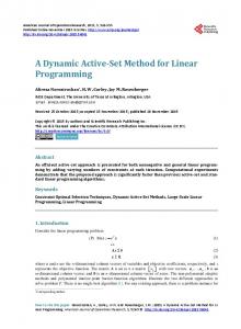
z
Infeasible
3x + y + 2z = 1 x, y, z ≥ 0
Ax = b
PSfrag replacements
y
x
PARA’04, June 22, 2004
Feasible
Solution
I. Idriss & W. V. Walter, Germany
6
Motivation and Goals 1. Primal-dual logarithmic barrier methods (Kojima, Mizuno & Yoshise, 1990) – currently the most efficient computational methods – simultaneous solution for [P] and [D] with duality gap c>x − b>y ≤ ² – If the starting point is infeasible, then the computed solution may be infeasible 2. Reliability of conventional computer program? – floating point arithmetic: roundoff error, cancellation, . . . – quality of approximate solution? – results occasionally qualitatively wrong Verified Computation • verification of existence and uniqueness of solution in an interval • guaranteed enclosure with narrow bounds for the optimal objective function value PARA’04, June 22, 2004
I. Idriss & W. V. Walter, Germany
7
Primal-Dual Logarithmic Barrier Methods Barrier Problems:
c>x − µ
Minimize
ln xi
i=1
subject to
Ax = b n X b>y − µ ln zi
Maximize
i=1
[Pµ]
[Dµ]
A> y + z = c
subject to Lagrangian Functions:
n X
L(x, y, µ) = c>x − µ
n X
ln xj − y >(Ax − b)
j=1
L(x, y, z, µ) = b>y + µ
n X
ln zj − x>(A>y + z − c)
j=1
PARA’04, June 22, 2004
I. Idriss & W. V. Walter, Germany
Primal-Dual Logarithmic Barrier Methods
8
Optimality Conditions Ax = b , A> y + z = c ,
[KKT]
XZe = µe , where X = diag(x1, x2, . . . xn) , Z = diag(z1, z2, . . . zn) , e = (1, 1, . . . , 1)> Iterative Solution ∆y = −(AXZ −1A>)−1AZ −1v(µ) , ∆z = −A>∆y , ∆x = Z −1v(µ) − XZ −1∆z , where v(µ) = µe − XZe PARA’04, June 22, 2004
I. Idriss & W. V. Walter, Germany
9
Mehrotra’s Predictor-Corrector Method • The goal is to follow the central path (x(µ), y(µ), z(µ)) • Predictor-corrector method proceeds as follows: correcting plane
(ˆ x, yˆ, zˆ)
PSfrag replacements (x1 , y 1 , z 1 )
(x0 , y 0 , z 0 )
PARA’04, June 22, 2004
Γ
Predictor
I. Idriss & W. V. Walter, Germany
10
A Verification Method LP as root finding problem
Ax − b
> F (x, y, z) = A y + z − c =0 XZe − µe Verification Problem u = (x, y, z), u = {(u1, u2, . . . , u2n+m)> ∈ IR2n+m | ui ≤ ui ≤ ui, 1 ≤ i ≤ 2n + m} Given: F : IIR2n+m → IIR2n+m Verify: There exists a unique u∗ ∈ u such that F (u∗) = 0
PARA’04, June 22, 2004
I. Idriss & W. V. Walter, Germany
A Verification Method
11
Techniques for Verification • Interval Arithmetic : ◦ ∈ {+, −, ·, /}, u , v ∈ IIR ◦ v = [5w, 4w] u, v ∈vv } = [w, w] ⊆ u ♦ u ◦v = {u ◦ v | u ∈u u) = {F (u) | u ∈ u } ⊆ F (u u) ⊆ F♦(u u) WF (u • Inclusion property:
u ⊆ u 0, v ⊆ v 0 ⇒ u ◦ v ⊆ u 0 ◦ v 0 u) ⊆ F (u u0) u ⊆ u0 ⇒ F (u
u) • Mean value form: u∗ = mid(u u)(u u − u∗), for u, u∗ ∈ u F (u) ∈ F (u∗) + JF (u • Brouwer’s fixed point theorem : Let u be a closed, bounded and convex u → u , then set in IRn and let F be a continuous mapping such that F :u F has a fixed point in u . u) ⊆ F♦(u u) ⊆ u ⇒ ∃ u ∗ ∈ u | u ∗ = F (u u∗) u ∈ IIRn : F (u PARA’04, June 22, 2004
I. Idriss & W. V. Walter, Germany
A Verification Method
12
A verification method can be defined by an iteration of the form: uk ) u ˜k = mid(u ¢ ¡ k −1 u ) R = mid JF (u
u, u u))(u u−u K(u ˜k+1) = u ˜ − R · F (˜ uk+1) + (I − R · JF (u ˜k+1) Some Notes 1. Under normal circumstances, every zero of F in u can be enclosed. 2. If there is no zero of F in u , the algorithm is generally able to prove this fact automatically in a finite number of iterations 3. Proof of existence or nonexistence of a zero of F in a given interval u occurs automatically: ◦ u, u • If K(u ˜) ⊂ u , then there exists a zero of F in u u, u • If K(u ˜) ∩ u = ∅, then there is no zero of F in u PARA’04, June 22, 2004
I. Idriss & W. V. Walter, Germany
13
Verified Linear Programming Algorithm (1) Let a primal problem [P] and its dual [D] be given (2) Compute an approximate solution (˜ x, y˜, z˜) for [P] and [D] by performing a primal-dual logarithmic barrier algorithm (3) Construct a small box u about the approximate solution u ˜ = (˜ x, y˜, z˜) by using an epsilon–inflation algorithm (4) Perform a verification step: (a) Prove the existence and uniqueness of a zero of F (b) Enclose the optimal objective function value by: c>x ∪ b>y
PARA’04, June 22, 2004
I. Idriss & W. V. Walter, Germany
14
Numerical Results Example 1
A=
µ
Iteration count
0 1 2 .. . 8 .. . 12 13
1 0 100
0 1 18
1 0 0
Primal objective
−0.59000000E −0.24989469E −0.32441434E .. . −0.24915636E .. . −0.25000000E −0.25000000E
0 1 0
0 0 1
¶ µ , b=
50 200 5000
Dual objective
+ 02 + 03 + 03 + 04 + 04 + 04
−0.52500000E −0.50203503E −0.49380485E .. . −0.25090225E .. . −0.25000000E −0.25000000E
and
c> = (−50, −9, 0, 0, 0)
Primal infeasibility
+ 04 + 04 + 04 + 04 + 04 + 04
0.49E 0.45E 0.43E .. . 0.17E .. . 0.32E 0.45E
+ 04 + 04 + 04 + 02 − 06 − 11
Dual infeasibility
Relative gap
0.51E + 02 0.47E + 02 0.45E + 02 .. . 0.17E + 00 .. . 0.34E − 08 0.50E − 13
0.52E + 04 0.48E + 04 0.46E + 04 .. . 0.17E + 02 .. . 0.34E − 06 0.48E − 11
Result of verification: Normal end, the problem has an optimal solution, an inclusion of the optimal value has been computed. [−2.5000000000000019E3,−2.4999999999999981E3] PARA’04, June 22, 2004
I. Idriss & W. V. Walter, Germany
Numerical Results
15
Example 2
A = (−1 Iteration count
0 1 2 .. . 8 9 .. . 14 15
Primal objective
0.30000000E 0.19091192E 0.25015137E .. . 0.27721815E 0.25064585E .. . 0.16550663E 0.62150694E
−1)
, b = (10−6)
Dual objective
+ 03 + 03 + 02 − 04 − 05 − 07 − 11
−0.10000000E −0.44436010E −0.13761119E .. . −0.78569105E −0.70012575E .. . −0.82880998E −0.41463218E
− 04 − 09 − 04 − 05 − 05 − 08 − 12
and
c=
³´ 2 1
Primal infeasibility
Dual infeasibility
Relative gap
0.20E + 03 0.13E + 03 0.18E + 02 .. . 0.26E − 04 0.74E − 05 .. . 0.22E − 07 0.98E − 11
0.60E + 01 0.38E + 01 0.53E + 00 .. . 0.79E − 06 0.22E − 06 .. . 0.66E − 09 0.30E − 12
0.30E + 03 0.19E + 03 0.25E + 02 .. . 0.36E − 04 0.95E − 05 .. . 0.25E − 07 0.66E − 11
Result of verification: The interval u contains no solution of F (u) = 0.
PARA’04, June 22, 2004
I. Idriss & W. V. Walter, Germany
Numerical Results
16
blend (NETLIB-test-problem with 75 equalities and 83 variables) Iteration count
0 1 2 .. . 10 11 .. . 24 25
Primal objective
−0.16500200E −0.40473968E −0.33415294E .. . −0.29243417E −0.29952535E .. . −0.30812150E −0.30812150E
Dual objective
+ 02 + 02 + 02 + 02 + 02 + 02 + 02
−0.11191000E −0.12064083E −0.11146155E .. . −0.31416758E −0.30708204E .. . −0.30812150E −0.30812150E
Primal infeasibility
+ 03 + 03 + 03 + 02 + 02 + 02 + 02
0.25E 0.21E 0.21E .. . 0.58E 0.20E .. . 0.11E 0.12E
+ 03 + 03 + 03 + 01 + 01 − 07 − 10
Dual infeasibility
Relative gap
0.10E + 03 0.87E + 02 0.85E + 02 .. . 0.24E + 01 0.84E + 00 .. . 0.44E − 08 0.56E − 11
0.95E + 02 0.80E + 02 0.78E + 02 .. . 0.22E + 01 0.76E + 00 .. . 0.39E − 08 0.20E − 12
Result of verification: Normal end, the problem has an optimal solution, an inclusion of the optimal value has been computed. [−3.0812149845852329E1,−3.0812149845852136E1]
PARA’04, June 22, 2004
I. Idriss & W. V. Walter, Germany
17
Conclusions • Our results indicate that the presented algorithm is robust. • A verification is obtained for all test problems. • The verification step is computationally the most expensive part of the algorithm. • The best choice of a default starting point is still very much an open question. • IPMs have been extended to more general classes of problems, but verified algorithms have not yet appeared.
PARA’04, June 22, 2004
I. Idriss & W. V. Walter, Germany