A versatile framework for simulating the dynamic mechanical - arXiv

A versatile framework for simulating the dynamic mechanical structure of cytoskeletal networks

arXiv:1609.05202v1 [physics.bio-ph] 16 Sep 2016

S. L. Freedman, S. Banerjee, G. M. Hocky, A. R. Dinner

Abstract Computer simulations can aid in our understanding of how collective materials properties emerge from interactions between simple constituents. Here, we introduce a coarsegrained model of networks of actin filaments, myosin motors, and crosslinking proteins that enables simulation at biologically relevant time and length scales. We demonstrate that the model, with a consistent parameterization, qualitatively and quantitatively captures a suite of trends observed experimentally, including the statistics of filament fluctuations, mechanical responses to shear, motor motilities, and network rearrangements. The model can thus serve as a platform for interpretation and design of cytoskeletal materials experiments, as well as for further development of simulations incorporating active elements.

1

1

Introduction

The actin cytoskeleton is a network of proteins that enables cells to control their shapes, exert forces internally and externally, and direct their movements. Globular actin proteins (G-actin) polymerize into polar filaments (F-actin) that are microns long and nanometers thick. Many different proteins bind to actin filaments. Crosslinkers are tens of nanometers in size and have multiple binding sites that enable them to connect actin filaments in networks that can transmit force. Myosins are comprised of head, neck, and tail domains and aggregate via their tails to form minifilaments that can attach multiple heads to actin filaments (1). Each myosin head can bind to actin and harness the energy from ATP hydrolysis such that a minifilament can walk along an actin filament in a directed fashion—i.e., it is a motor. These dynamics have been extensively studied, and it is well understood how they give rise to muscle contraction, for example. In muscle cells, actin filaments are arranged in parallel bundles called sarcomeres. A myosin II minifilament binds to two antipolar sarcomeres, walks toward the barbed end of both, and the tension along the myosin pulls the sarcomeres together (2). In other types of cells that lack this level of network organization, however, the ways in which the elementary molecular dynamics act in concert to give rise to complex cytoskeletal behaviors remains poorly understood. Addressing this issue requires a combination of experiment, physical theory, and accurate simulation. The last of these is our focus here—we present a non-equilibrium molecular dynamics simulation that can be used to efficiently explore the structural and dynamical state space of assemblies of semiflexible filaments, molecular motors, and crosslinkers. By allowing independent manipulation of parameters normally coupled in experiment, this computational model can guide our understanding of the relationship between the microscopic biochemical protein-protein interactions and the macroscopic mechanical functionalities of assemblies. Additionally, because the model simulates filaments, motors, and crosslinkers explicitly, we can study its stochastic trajectories at levels of detail that are experimentally inaccessible to elucidate microscopic mechanisms. In this work we detail the model and demonstrate that, with a single set of parameters, it reproduces an array of known experimental results for actin filaments, assemblies of actin and crosslinkers (passive networks), and assemblies of actin and myosin (active networks). We go further to provide new experimentally testable predictions about these systems. For single polymers, we reproduce the spatiotemporal fluctuation statistics of actin filaments. For passively crosslinked networks, we reproduce known stress-strain relationships and predict the dependence of the shear modulus on crosslinker stiffness. For active networks, we reproduce velocity distributions of actin filaments in myosin motility assays and show how one can tune their dynamical properties by varying experimentally controllable parameters. In a separate study, we apply the model to investigating how assemblies of actin filaments and crosslinkers can be tunably rearranged by myosin motors to form structures with distinct biophysical and mechanical functionalities (Freedman, S.L., S. Banerjee, G.M. Hocky, and A.R. Dinner, in preparation). The collection of this benchmark suite is itself useful, as prior models (3–13) have focused on specific cytoskeletal features, making the tradeoffs needed to capture the selected behaviors unclear. Indeed, our model builds on earlier studies, which we briefly review to make clear similarities and differences of the models (see also (14) for a list of cytoskeletal simulations). The most finely detailed simulations focus on the motion of a myosin minifilament with respect to a single actin filament. Erdmann and Schwarz (8) used Monte Carlo simulations to verify a master equation describing the attachment of a minifilament and, in turn, the duty ratio and force 2

velocity curves as functions of the myosin assembly size. Stam et al. (15) used simulations to study force buildup on a single filament by a multi-headed motor and found distinct timescale regimes over which different biological motors could exert force and act as crosslinkers. These models of actin-myosin interactions are important for understanding the mechanics at the level of a single filament, and their results can be incorporated into larger network simulations. A number of publications have dealt with understanding the rheological properties of crosslinked actin networks (3–6). For example, to study the viscoelasticity of passive networks, Head et al. (4) distributed filaments randomly on a two-dimensional (2D) plane, crosslinked filament intersections to form a force-propagating network, sheared this network, and let it relax to an energy minimum, corresponding to a quasistatic equilibrium. From this model, they were able to identify three elastic regimes that were characterized by the mean distance between crosslinkers and the temperature. Dasanyake and coworkers (7) extended this model to include a term in the potential energy that corresponded to myosin motor activity and observed the emergence of force chains that transmit stress throughout the network. These studies address questions about how forces propagate and how crosslinker densities alter mesh stiffness. Other studies characterized network structure and contractility as functions of model parameters. Wang and Wolynes (9) considered a graph of crosslinkers (nodes) and rigid filaments (edges) in which motor activity was simulated via antisymmetric kicks along the filaments. They calculated a phase diagram for contractility as a function of crosslinker and motor densities. Such a simulation can provide qualitative insights into general principles of filament networks, but the model did not account for filament bending, and structures were sampled via a Monte Carlo scheme that was not calibrated to yield information about dynamics. Cyron et. al. (16) used Brownian dynamics simulations to investigate structures that can form via mixtures of semiflexible filaments and crosslinkers and determined a phase diagram and phase transitions (17) between differently bundled actin networks that form as one varies crosslinker density and crosslinker-filament binding angle. Nedelec and coworkers performed dynamic simulations of assemblies of semiflexible microtubules and kinesin motor proteins, which share features with assemblies of F-actin and myosin; they used their simulation package, CytoSim, to understand aster and network formation in microtubule assays (10) and showed recently that the model can be adapted to treat actin networks (11). Gordon et al. (12), Kim (13), and most recently Popov et al. (14) similarly simulated dynamics of F-actin networks and included semiflexible filaments, motors and crosslinkers. By varying motor and crosslinker concentrations, Gordon et al. (12) and Popov et al. (14) showed various structures that can emerge from assemblies of this type, and Kim (6, 13) additionally quantified how these changes could effect force propagation within the network. We have strived to include many of the best features of these preceding models in our simulations. We use the potential energy of Head et al. (4) for filament bending and stretching. However, in contrast to (4, 7), which simply relax the network, we simulate the stochastic dynamics, including thermal fluctuations, crosslinkers and myosins binding and unbinding, and the processive activity of myosin. The force propagation rules and kinetic equations for binding and unbinding are similar to those of (10, 12), while the length and time scales simulated echo those performed in (11, 13). We expand on these works by combining and documenting key elements in a single model, demonstrating that the model can capture experimentally determined trends for cytoskeletal materials quantitatively, and illustrating how the model can be used to study systems of current experimental interest.

3

2

Materials and Methods

To access time and length scales relevant to network reorganization, we represent actin filaments, myosin minifilaments, and crosslinkers in a coarse-grained fashion (Fig. 1A). We model actin filaments as polar worm-like chains (WLC) such that one end of the WLC represents the barbed end of a filament and the other its pointed end. We model crosslinkers as Hookean springs with ends that can bind and unbind from filaments. Thus, the connectivity of a network and, in turn, its capacity for force propagation can vary during simulations. We model molecular motors similarly to crosslinkers except that each head bound to a filament can walk toward a filament end in a load-dependent fashion. The motors can slide filaments, translocate across filaments, and increase network connectivity. We simulate the system with Langevin dynamics in 2D because the in vitro experiments we wish to interpret are quasi two-dimensional and approximating the system as 2D allows us to treat larger systems for longer times. To account for the fact that a three-dimensional (3D) system would have greater conformational freedom, we do not include steric interactions for our filaments, motors and crosslinkers. This implementation of filaments, motors and crosslinkers, which we detail below, allows for motor-driven filament sliding and filament buckling, as seen in Fig. 1D-E. A complete list of model parameters, their values, and sources is given in Table 1. kcloff

A

B k ,l ,κ a a B

θi

θi+1

θi-1

v0

E

D kclon

0s

C rc

3s

10s Figure 1: Overview of the model. See Section 2 for details. (A) Schematic of a configuration of the model. Filaments are red, crosslinkers are green, and motors are black. (B) Expanded view of the actin filament representation: a chain of beads connected by springs with spring constant ka , rest length la , and bending modulus κB , as detailed in Section 2.1. (C) The process by which a crosslinker binds to a filament, as detailed in Section 2.2. The solid red link is indexed to the grid points marked with either red or purple stars, and the solid green motor head searches the grid points marked with either green or purple stars for links to bind. The motor head then stochastically binds to the nearest spot on the filament, here marked with a purple ×. (D) Successive images of two antiparallel 10 µm filaments (barbed end marked in blue) interacting with one motor at the center. The motor binds to both filaments and slides them past each other. (E) Similar to (D) but with a crosslinker that pins the top filament’s pointed end to the bottom filament’s barbed end. The motor, bound to both, walks toward the barbed end of the bottom filament and buckles the top filament.

4

2.1

Filaments

The WLC model for actin filaments is implemented as a chain of N + 1 beads connected by N harmonic springs (links) and N − 1 angular harmonic springs, as depicted in Fig. 1B. The N linear springs penalize stretching and keep the filament’s average end-to-end length constant. The N − 1 angular springs penalize bending and fix the persistence length for a free filament. The filament configurations are governed by the potential energy Uf : Uf = Ustretch + Ubend Ustretch Ubend

N ka X (|~ri − ~ri−1 | − la )2 = 2 i=1

(1)

N κB X 2 = θ , 2la i=2 i

where ~ri is the position of the ith bead on a filament, θi is the angle between the ith and (i − 1)th links, ka is the stretching force constant, κB is the bending modulus, and la is the equilibrium length of a link. In practice, Uf enters the simulation through its Cartesian derivatives (i.e., the forces—see Eq. (7) below). In this regard, it is important to note that linearized forms for the bending forces are employed in the literature (10), but we found that it was necessary to use the full nonlinear force to obtain consistent estimates for the persistence length, Lp (Section 4.1). We thus employ the full nonlinear Cartesian forces throughout this work, using the expressions in Appendix C of (18). It has been shown that for a confined semiflexible filament with a persistence length Lp , the 1/3 shortest length that should be considered as unbending (la ) is given by la ≈ A2/3 Lp where A is a length scale associated with the confinement (19). In these simulations, filaments were restricted by nearby motors and crosslinkers. Since the largest motorp or crosslinker density that −2 we consider is ρm = 10 µm , the confinement length scale A ≥ 1/ 10 µm−2 . Therefore, for the free-filament persistence length of Lp ≈ 17 µm (20), the filament subunit can be as large as la = 1.19 µm; we used la = 1 µm (Table 1). The bending force constant is also derived from the persistence length Lp such that κB = Lp kB T , where kB is Boltzmann’s constant, and T is the temperature (21). The experimentally measured force constant is ka = 55 ± 15 pN/nm (22, 23). However, simulating a network of such stiff filaments is computationally infeasible since the maximum time step of a simulation is inversely proportional to the largest force constant in the simulation (24). Therefore, we set ka to a smaller value than measured. However, because ka  κB /la still, filaments prefer bending to stretching, and, as we show, the ability to capture network properties quantitatively is not compromised.

2.2

Crosslinkers

There are a variety of different actin binding proteins that serve as crosslinkers. Crosslinkers connect filaments dynamically and propagate force within the network. Thus, the crosslinkers in our model must be able to attach and detach from filaments with realistic kinetic rules and be compliant when bound. To this end, we model them as Hookean springs with stiffness kxl and rest length lxl . Like actin filaments, the Young’s modulus of most crosslinkers is significantly higher than would be reasonable to simulate; therefore, for network simulations without large external forces, we set kxl = ka so that the bending mode of actin filaments was significantly 5

softer than the stretching mode of crosslinkers. The rest length lxl corresponds to the size of the crosslinker and therefore differs based on the particular actin binding protein one wishes to study. At each time step of the simulation an unattached crosslinker end (head) is allowed to attach to nearby filaments and an attached crosslinker head can detach. Crosslinkers are modeled as slip bonds, and detachment follows Bell’s law, so that a higher tensile force along the crosslinker backbone results in a higher probability of detachment (25): of f ∆t exp (max{Txl , 0}/Fxlrup ), Pxlof f = kxl

(2)

of f where kxl a the unloaded detachment rate, ∆t is the simulation timestep, Txl is the tension along the crosslinker backbone, and Fxlrup is the force required to rupture the bond that a crosslinker forms between two actin filaments (26). The probability of a head attaching to an actin filament is a Gaussian distributed random variable, such that on B Pxlon = kxl ∆t exp(−3kxl |~rxl − ~ra |2 /2Uxl ), (3) on is the maximum on rate, ~rxl is the crosslinker head position, ~ra is the attachment where kxl B is the binding energy of the crosslinker. The attachment point on the actin filament, and Uxl point ~ra is the point on a filament link that minimizes the distance between that link and the crosslinker head. Because the probability of attachment drops off exponentially as |~rxl − ~ra |2 , it is highly inefficient for a crosslinker to attempt attachment p to every filament link in the B simulation box. Rather, we determine a cutoff distance rc = Uxl /kxl (corresponding to three times the standard deviation of the Gaussian in Eq. (3)) so that if the distance between a motor and a filament is greater than rc the probability of attachment is zero. This allows us to use the following neighbor list scheme, illustrated in Fig. 1C, to determine crosslinker-filament attachment. A grid of lattice size of at least rc is drawn on the 2D plane of the simulation, and each filament link is indexed to the smallest rectangle of grid points that completely enclose it. In practice the lattice size is generally larger than rc due to memory constraints, and is denoted by the model parameter g, the number of grid points per µm in both the x and y directions. Since a crosslinker head cannot bind to a filament link for which |~rxl − ~ra | > rc , it suffices for a crosslinker head to only attempt attachment to the nearby filament links indexed to its four nearest grid points. The crosslinker then chooses, via Monte Carlo, to attach to the ith nearby P link with probability Pxlon (~ra,i ) or not to attach at all with probability 1 − i Pxlon (~ra,i ). When both crosslinker heads are attached to filaments, the crosslinker is generally stretched or compressed. We propagate the tensile force stored in the crosslinker onto the filaments via the lever rule outlined in (12, 27). Specifically, if the tensile force of a crosslinker head at position ~rxl between filament beads i and i + 1 is F~xl , then, ~rxl − ~ri F~i = F~xl ~ri+1 − ~ri (4) ~ ~ ~ Fi+1 = Fxl − Fi

are the forces on beads i and i + 1 respectively due to the crosslinker.

2.3

Motors

In the present work, we focus on the motor myosin II. As mentioned above, tens of myosin II proteins aggregate into bipolar assemblies called myosin minifilaments (15). For both myosin 6

minifilaments, and monomeric myosin, motility assay experiments have shown that on average bound myosin heads walk toward the barbed end of actin filaments at speeds in the range 0.2 − 4 µm/s (28–31). Since myosin also functions to increase the local elasticity of networks wherever it is bound, we model a motor similarly to a crosslinker, in that it behaves like a Hookean spring with two heads, a stiffness km and a rest length lm . The two heads of this spring do not correspond directly to individual myosin protein heads; rather each of them represents tens of myosin molecules. Experimentally minifilaments have a very high Young’s modulus, and it is unlikely that their lengths change noticeably in cytoskeletal networks. As with the passive crosslinkers, we set km = ka so that the bending of actin is still the softest mode. The rest length was set to the average length of minifilaments, lm = 0.5 µm (1). Attachment and detachment kinetics, as well as force propagation rules for motors are the same as for crosslinkers, subscripted with m instead of xl in Eqs. (2) to (4). Unlike crosslinkers, motors move towards the barbed end of actin filaments to which they are bound at speeds that linearly decrease with tensile force along the motor. The motor head therefore is fastest if the minifilament is compressed and slowest if the minifilament is stretched. The speed goes to zero when the force on the minifilament exceeds the stall force, Fs ≈ 10 pN (12, 27), and therefore can be modeled as a piecewise linear function of the force; i.e.,   F|| (5) v(F|| ) = v0 max 1 − , 0 , Fs where F|| is the force on the motor head, projected along the tangent vector of of the actin filament to which it is attached. The minor differences between crosslinkers and motors allow us treat them with equivalent objects within the program, setting v0 = 0 for the crosslinkers.

2.4

Dynamics

We use overdamped Langevin dynamics to solve for the motion of filament beads, motors, and crosslinkers. The Langevin equation of motion for a spherical bead of mass m, radius R at position ~r(t) at time t, forced by F~ (t) is ~ − 4πRν ~r˙ (t), m~r¨(t) = F~ (t) + B(t)

(6)

~ where B(t) is a Brownian forcing term that introduces thermal energy, ν is the dynamic viscosity of the bead’s environment, and we use the Einstein relation for the damping term. Since the fastest motion in this simulation is that of the myosin, and a 0.4 µm myosin minifilament moving at a speed of 1 µm/s in a liquid at least as viscous as water (with dynamic viscosity νD = 106 µm2 /s) has a very low Reynolds number (Re ≈ 4 × 10−7 ), we treat the dynamics as overdamped and set m = 0 in Eq. (6). Furthermore, in the limit of small ∆t, we may write ~r˙ (t) ≈ (~r(t + ∆t) − ~r(t))/∆t. These two approximations allow us to rewrite Eq. (6) as ~ ~r(t + ∆t) = ~r(t) + F~ (t)µ∆t + B(t)µ∆t

(7)

where µ = (4πRν)−1 . For the Brownian term, we use the form of Leimkuhler and Matthews (32): s ! ~ (t) + W ~ (t − ∆t) 2k T W B ~ , (8) B(t) = µ∆t 2 ~ (t) is a vector of random numbers drawn from the normal distribution N (0, 1) × where W N (0, 1). This numerical integrator minimizes deviations from canonical averages in harmonic 7

systems; given that the all the mechanical forces in our model are harmonic, we expect this choice to yield accurate statistics in the present (athermal) context as well. The value for ∆t in Eq. (7) is most strongly dependent on the largest force constant in the simulation, kf , but also depends on other simulation parameters, such as v0 , k on and k of f for both motors and crosslinkers. Table 1 can be used as a rough guide for how high one can set the value of ∆t for a given set of input parameters; e.g., for a the contracting network where ka = 1 pN/µm, of f of f on on = km = 0.1 s−1 a value of ∆t = 0.00002 s was v0 = 1 µm/s, kxl = km = 1 s−1 , and kxl just low enough to iteratively solve Eq. (7) without accumulating large error.

2.5

Environment

In general we use periodic boundary conditions so as to limit effects of a boundary and to mimic a system larger than the one that we simulate. We implemented square boundaries to model enclosed systems, as well as Lees-Edwards boundaries for shearing simulations (18). The dimensions of the simulation box (Table 1) were chosen to be five times the contour length of filaments so as to be large enough to avoid boundary artifacts due to the self-interaction of constituent components.

3

Implementation

The model is implemented as an open source C++ package called Active Filament Network Simulation (AFiNeS) that is available at http://www.dinner-group.uchicago.edu/downloads.html. Installation instructions are available in the README file in the top directory of the AFiNeS package. To run a simulation, a user must compile the code into an executable (e.g., with the provided Makefile), and create the output directories. A user can set parameters using commandline arguments or a file. For example, if the user has compiled the code into the executable “afines”, created the output directories “test/txt stack” and “test/data”, and wants to run a simulation of 500 15 µm actin filaments, interacting with 5 motors/µm2 , and 1 crosslinker/µm2 , in a cell that is 75 µm × 75 µm, for 100 s, he or she could issue the following command afines --xrange 75 --yrange 75 --npolymer 500 --nmonomer 16 \ --a_motor_density 5 --p_motor_density 1 --tf 100 --dir test Alternatively, the user could write the following to the file my config.cfg xrange=75 yrange=75 npolymer=500 nmonomer=16 a_motor_density=5 p_motor_density=1 tf=100 dir=‘‘test’’ and then run the code using the command afines -c my_config.cfg 8

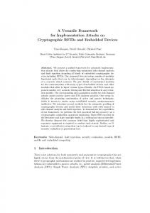
When all other parameters were left as defaults (see README file for full list of program parameters), the executable was compiled using g++ with the -O3 optimization flag, and the simulation was run on an Intel E5-2670 node with 2 Gb of memory and a 2.6 GHz processor, this example finished in less than 3 days of wall clock time. In general, the simulation scales linearly with system size, as seen from Fig. 2.

A

C

B

t-1

t t2

t

t-2

Figure 2: Wall clock time for a 10000 step simulation with step size ∆t = 0.0001 s. (A) For a constant system size, run time scales linearly or sub-linearly as both filament density (red dots) and motor density (blue dots) are increased independently. If both are increased together (black dots), a quadratic scaling is approached for large numbers of particles. (B) At constant motor and filament density, run time scales linearly with system size XY . (C) At constant system size, run time decreases with increasing grid density g, and thereby the number of neighbor-list grid elements g 2 XY used to calculate motor-filament interactions. Grids more dense than 2 µm−1 exceeded the system’s memory capacity. All benchmarks are for an Intel E5-2670 node with 2 Gb of memory and a 2.6 GHz processor.

9

Table 1: Parameter Values

Symbol

Description (units) [references] Lp

ρxl lxl

Actin Filaments Number of filaments Number of beads per filament Link rest length (µm) (19) Stretching force constant (pN/µm) Bending modulus (pNµm2 ) (20) Myosin Motors Motor density (µm−2 ) Rest length (µm) (1) Stiffness (pN/µm) Attachment rate at distance r = 0 (s−1 ) Detachment rate at 0 tension (s−1 ) Binding energy (pN µm) Rupture force (pN) Unloaded speed (µm/s) (28) Stall force of myosin (pN) (33) Crosslinkers Crosslink density (µm−2 ) Rest length (Filamin) (µm) (26)

kxl

Stiffness (pN/µm)

n/a

Attachment rate at distance r = 0 (s−1 ) Detachment rate at 0 tension (s−1 ) Binding energy (pN µm) Rupture force (pN) (26) Environment

n/a n/a n/a n/a

Nf NB la ka κB ρm lm km on km of f km B Um Fmrup v0 Fs

on kxl of f kxl B Uxl rup Fxl

∆t TF X, Y g T ν ∆γ trelax

4

Dynamics timestep (s) Total simulated time (s) Length and width of assay (µm) Grid density (µm−1 ) Temperature (K) Dynamic viscosity (mg/(µm×s)) Strain (%) (34) Time between sequential strains (s)

Simulation Motility Shear Assay

Network

1 [21, 201] 1 [0.01, 10] [0.002, 5]

500 16 1 1000 0.08

1 16 1 1 0.08

500 11 1 1 0.08

n/a n/a n/a n/a n/a n/a n/a n/a n/a

n/a n/a n/a n/a n/a n/a n/a n/a n/a

[0.0, 10] 0.5 1 [0.001, 2] 1 0.04 10 1 10

0.2 0.5 1 1 0.1 0.04 10 1 10

n/a n/a

0.42 0.150

n/a n/a

1 0.150

n/a

1

n/a n/a n/a n/a

1 0.1 0.04 10

10−7

0.00005

0.00002

0.5 75 n/a 300 0.001 0.001 0.001

1000 50 1 300 0.001 n/a n/a

200 50 1 300 0.001 n/a n/a

10−5 , 10−4 2000 n/a n/a 300 0.001 n/a n/a

[0.1, 1000] 1 0 0.04 10

Results and Discussion

In this section, we numerically integrate the model to obtain stochastic trajectories and compare their statistics to both known analytical results for semiflexible polymers and networks, as well as experimental observations.

10

4.1

Actin Filaments Exhibit Predicted Spatial and Temporal Fluctuations

The persistence length of a semiflexible filament with bending modulus κB is expected to be Lp = κB /kB T , where kB is Boltzmann’s constant, and T is the temperature. However, when simulating the dynamics, approximations can enter both the evaluation of the forces and the discretized numerical integration of the equations of motion. Because the persistence length is a measure of filament fluctuations, and not an input to the simulation, its dependence on simulation features must be determined empirically, and, as discussed in Section 2.1 and further below, some care is required to obtain reliable estimates of Lp . For a two dimensional filament composed of links d~1 . . . d~N (d~i = ~ri − ~ri−1 ) with a constant link length la , constant total contour length L, and where a small bend of link d~i with respect to link d~i−1 results in a local change in free energy of (κB /2la )θi2 , it is possible to show analytically that (35) hθ2 (l)i = l/Lp (9) hcos(θ(l))i = exp (−l/2Lp ),

(10)

where θ(l) = θj − θi (1 < i < j ≤ N ), l = la (j − i) and Lp is the persistence length. To test our WLC model against these predictions, we let 100 filaments of L = 200 µm and κB = 0.08 pNµm2 fluctuate at T = 300 K for Tf = 100 s and measured the resulting filament configurations. The configurations saved were chosen to be 1 s apart, since the decorrelation time for θ(l) was at most 0.64 s (see Section S1 and Fig. S1 for details). The first 10 s of each simulation was disregarded as filaments had not yet equilibrated, and the first and last 25 µm of each filament were disregarded to avoid end effects, which we found to be significant. For each of the 90000 filament configurations saved, and for each l ∈ 0, 1, 2, .., 150 µm, θ2 (l) and cos(θ(l)) were calculated. Their respective averages are plotted in Fig. 3B, along with the expected behavior given the input κB .

11

A

λ

B

C 1 0.1 0.01 0.001 0.001

0.01

0.1

1

Figure 3: Spatial and temporal fluctuations of the bead-spring WLC. (A) Schematic of a filament and the order parameters that characterize its fluctuations. Spatial fluctuations are characterized by the angle between two tangent vectors ~vs and ~vs+l along the filament as a function of the contour length between them l. Temporal fluctuations are characterized by the eigenvalues λ1,2 (t) of the covariance matrix of filament endpoint positions as a function of time. The red arrow indicates the larger moment (size of transverse fluctuations) while the blue arrow indicates the smaller moment (size of longitudinal fluctuations). (B) Decorrelation of tangent vectors (red circles) and fluctuations in angles between links (blue circles) as a function of the arc length between them. Dashed lines show expected behavior for κB = 0.08 pNµm2 . (C) Eigenvalues of covariance matrices for the positions of endpoints of filaments as a function of time (36). Red dots show the large eigenvalue λ1 (t), which is expected to be proportional to t3/4 (red line) while blue dots show λ2 (t), expected to be proportional to t7/8 (blue line).

As alluded to above, the numerical integration can make the persistence length depend on simulation parameters in non-obvious ways. Consequently, we measured the sensitivity of Lp to independent variations of κb , la , and ka . The results shown in Fig. 4 are obtained from the “blue” method in 3(B), where, following Eq. (9), Lp = 1/(dhθ2 (l)i/dl). Fig. 4A shows that in the range of κB ∈ [5, 500]µm×kB T , Lp corresponds well with the input bending modulus, and can be easily tuned to simulate filaments of varying rigidity. Fig. 4B shows that for a link stiffness ka > 0.2 pN/µm, Lp is independent of ka . Fig. 4C shows that the most consistent values of Lp are obtained when la ∈ [0.5, 5] µm, which overlaps with the prediction of la ≈ 1 µm described in Section 2.1. We thus see that, while there is a range in which Lp is independent of the filament link parameters, ka and la , extreme values for those parameters also effect Lp .

12

A

C

B

Figure 4: Dependence of the persistence length on the parameters for numerically integrated semiflexible filaments. (A) ka = 1pN/µm and la = 1µm. (B) κB = 20 µm×kB T and la = 1µm. (C) κB = 20 µm×kB T and ka = 1 pN

The statistics of temporal fluctuations are also known for semiflexible filaments. Fluctua2 i ∝ t3/4 , while longitudinal fluctions transverse to the filament orientation increase as hdr⊥ tuations increase as hdr||2 i ∝ t7/8 (36). To determine if our simulations conformed to these theoretical scalings, we followed the procedure outlined in (36) and generated N = 100 initial filament configurations of a 20 µm filament. This length was chosen because it satisfied the constraint provided in (36) for the fluctuations of the two ends of the filament to be uncorrelated at long times (here t = 1 s); i.e., 20 µm> (tkB T /ν)1/8 (κB /kB T )5/8 . For each configuration we ran M = 100 simulations of the filament diffusing freely for 1 s. We denote each of the the M positions for each endpoint at each time by ~re (t). For each of the clouds of points shown in Fig. 3C, we calculated the moments, as the eigenvalues of the covariance matrix with elements h(~re (t) · ˆi − h~re (t) · ˆii)(~re (t) · ˆj − h~re (t) · ˆji)i for i, j ∈ {x, y}. The larger eigenvalue λ1 (t) corresponds to the transverse fluctuations (i.e., λ1 (t) ∝ t3/4 ) while the smaller eigenvalue corresponded to longitudinal fluctuations (λ2 (t) ∝ t7/8 ). We show these results in Fig. 3D. Each point is the average over the 2N eigenvalues for λ1 (t) and λ2 (t), and the error bars indicate standard deviations. As seen, the calculated scalings are in good agreement with the predicted behaviors.

4.2

Tunable elastic behavior of crosslinked filament networks

The mechanical properties of crosslinked F-actin have important ramifications for force generation and propagation within a cell, and are generally inferred using rheological measurements of in vitro networks (37–40). In a typical experiment, actin and crosslinker proteins are mixed to form a crosslinked mesh and then sheared in a rheometer by a prestress, σ0 . The prestressed network then undergoes a sinusoidal differential stress of magnitude dσ  σ0 . By measuring the resulting strain, one can calculate the differential elastic modulus G(σ0 ) = dσ/dγ. Results from such experiments indicate that, in contrast to a purely viscous fluid, crosslinked F-actin networks resist shear, but, unlike a simple solid, their elasticity is nonlinear. In particular, they are shear stiffening, meaning G increases with increasing stress. In experiments using a stiff crosslinker, such as scruin, the dependence of the differential 3/2 modulus on high prestress is G ∝ σ0 (37, 40). Force-extension experiments with semiflexible filaments, in which one directly measures the force F required to extend a filament by a distance l, yield a remarkably similar relationship, dF/dl ∝ F 3/2 (41, 42). As remarked in (37), this suggests that their shear stiffening is a direct result of the nonlinear force-extension relationship of actin. Rheology studies using more compliant crosslinkers, such as filamin, have found a softer response, G ∝ σ0 , indicating that a significant amount of stress is mediated through the 13

crosslinkers, and not the filaments (39). These results suggest that the strain stiffening behavior of a crosslinked network can be tuned by varying the crosslinker stiffness. To test this possibility and benchmark our simulations, we subjected passive networks comprised of filaments and crosslinkers to shear. We initialized each simulation with N = 500 randomly oriented filaments of length 15 µm in a square box of area 75 µm × 75 µm. A 0.150 µm crosslink (corresponding to the length of filamin) was initially placed at each filament intersection. To inhibit network restructuring, the detachment rate of the crosslinkers was set to zero. We performed 24 such simulations, each with a different crosslinker stiffness ranging from 0.1 − 1000pN/µm. Simulating the experimental shear requires modifying the equations of motion and the periodic boundary condition to achieve a planar Couette flow. In general, planar Couette flow can be simulated via molecular dynamics using Equation 4.1 in (43): m¨ x = Fint,x + γy ˙ m¨ y = Fint,y ,

(11)

where x and y are the Cartesian coordinates of a particle being sheared, Fint,x , Fint,y are the internal forces on those particles and γ is the strain. Simultaneously, the upper and lower boundaries must be sheared by the total strain on the simulation box (18). Comparing Eq. (11) with Eq. (6) for Langevin dynamics, we can substitute Fint,x = Fx (t) + Bx (t) − 4πRν x(t). ˙ With the additional Brownian dynamics approximation of x¨i = 0, implementing Eq. (11) is equivalent to updating filament bead positions via Eq. (7), and shifting the horizontal position of a bead (xi ) by y  i (12) xi → xi + ∆γ Y where ∆γ = ∆tγ˙ and Y is the simulation cell height. The boundary conditions follow the Lees-Edwards convention (18). Since moving the particles ∆γ is equivalent to the addition of a significant external force on the system, it is necessary to let the network relax for a specified amount of time trelax after each shear event, before measuring the network’s internal energy. The magnitude of trelax depends on ∆γ, which in turn depends on the desired discretization of the shear and the timestep ∆t. As shown in Section S1.2 and Fig. S2, we found that ∆γ = 0.001, ∆t = 10−7 s, and trelax = 0.001 s yielded a stable planar Couette flow, with high enough strains to observe strain stiffening. This protocol was performed for Tf = 0.5 s allowing the total strain to reach a value: γ = ∆γTf /trelax = 0.5. We measured the elastic behavior of the network for each crosslinker stiffness by calculating w, the strain energy density at each timestep: ! X X 1 Uf + Uxl , (13) w(t) = XY f xl where Uf is the mechanical energy of individual filaments (Eq. (1)) and Uxl = (kxl /2)(∆lxl )2 is the mechanical energy of each crosslink. By averaging over windows of size trelax , we determine w(γ). Fig. 5 shows the results of these calculations for various values of kxl . For extremely low kxl , the strain energy scaled linearly with strain, w ∝ γ, indicating that the network showed no resistance to shear: G = d2 w/dγ 2 = 0. For high kxl , we observe a neoHookean strain stiffening behavior, w → γ 4 (44). Thus, one can tune the behavior of these networks from being liquid-like, with w ∝ γ, through the Hookean elastic regime of w ∝ γ 2 14

up to the strain stiffening regimes of w ∝ γ 3 and w ∝ γ 3.5 , previously reported in experiments (37, 39).

A

B

γ=0.1

U(pNμm)

γ=0.25 γ=0.5

D

C

γ3.5 γ2

Figure 5: Tunable elasticity of crosslinked networks. (A) Snapshots of a strained network (ka = kxl = 1000 pN/µm) at γ = 0.1, γ = 0.25, and γ = 0.5. Color indicates stretching energy on each link, with green being the lowest and yellow being the highest. For all snapshots, t = γ × 1 s. (B) The potential energy of the network as a function of time shown at different strains γ0 = 0.1 (circles), γ0 = 0.25 (squares), and γ0 = 0.4 (triangles), where t0 = γ0 × 1 s. Black dashed line shows the strain protocol. (C) Strain energy density (w = U/area) for various values of crosslinker stiffness kxl . Blue dashed line indicates expected behavior for a linearly elastic solid (w ∝ γ 2 ) and green dashed line indicates strain stiffening behavior of w ∝ γ 3.5 as expected for semiflexible polymer networks (37, 40). (D) Power-law exponent of w(γ), evaluated via least squares fit to ln γ as a function of ln w.

4.3

Ensembles of motors interacting with individual filaments simulate actin motility assays

While the force dependent detachment and speed of an individual myosin motor is a model input (Sections 2.2 and 2.3), the action of many motors on a filament is an output that can be compared with actin motility assays (45, 46). In a classic motility assay, a layer of myosin is adhered to a plate, and actin filaments are placed on top of the motors. Because the myosin molecules cannot move, they slide the actin filament. The speed of an actin filament has been reported to depend nonlinearly on the concentration of myosin and the concentration of ATP in the sample (29, 30). By allowing filaments to interact with more motors, one can monotonically increase the filament speed to a constant value. To explore the dynamics of this assay, we randomly distributed motors on a 50 µm ×50 µm periodic simulation cell and tethered one head of each motor to its initial position. Filaments were then introduced in the simulation cell and allowed to interact with the free motor heads. The strength of motor-filament interactions was manipulated in three ways: by varying the on on motor concentration ρm , the filament contour length L, and the duty ratio rD = km /(km + of f km ). While L and rD are difficult to modulate experimentally in a well-controlled fashion, 15

as they require the addition of other actin-binding proteins to the assay, they are predicted to impact the dynamics of actin because they affect the number of myosin bound to an actin filament at any one time (30). Since they are both simple functions of the model’s parameters, we were able to test this hypothesis directly. The results are shown in Fig. 6, where we have used the dimensionless control parameter M = ρm lm LrD (where ρm lm is the linear motor density) representing the average number of bound motor heads, to tune filament motility. Our findings are qualitatively similar to the previously reported experimental results and expand on them by collapsing the trends observed while varying ρm , L and rD into a single effective parameter. At low M, i.e., low motor density, filament length, or duty ratio, Fig. 6B shows that transverse motion dominates over longitudinal motion as the filament is not propelled by motors faster than diffusion, and transverse filament fluctuations are larger than longitudinal fluctuations (consistent with Fig. 3C). However, as M is increased, longitudinal motion dominates. The longitudinal speed of the filament plateaus at v|| ≈ 1 µm/s which is the input unloaded speed of a single motor head and closely matches experimental results (28, 30). We directly relate the increase in longitudinal filament speed by plotting the mean squared displacement (MSD) of the filament in Fig. 6C defined as h∆r2 i where ∆r(t) = |~r(t + δt) − ~r(t)| and angle brackets indicate an average over time t. We show that low M yields diffusive behavior with h∆r2 i ∝ δt, and high M yields ballistic motion with h∆r2 i ∝ δt2 . A striking feature of these simulations was how the direction of a filament changed over time. Experimentally this has been studied at high actin density and self-organization patterns emerge (47). However, to the best of our knowledge this characteristic of motility assays has not been studied for single actin filaments. To quantify the effect of varying M on the length of time that a filament moves in the same direction, we calculate the autocorrelation of the orientation of the (N + 1)-bead filament, ~rN 0 = ~rN − ~r0 , as described in Section S1.3. Fig. 6D shows the integrated autocorrelation time of ~rN 0 as a function of M. For a wide range of parameter choices the autocorrelation time is approximately 15 s, which, for the green and blue curves (L = 15 µm) is the maximum amount of time a motor (vm = 1 µm/s) can walk on an unloaded filament. For the red curve, L = M × 1 µm can be greater than 15 µm, but ~rN 0 decorrelates at distances on the order of the persistence length Lp = 20 µm owing to filament fluctuations. Additionally, Fig. 6D shows that lowering the motor density or the duty ratio increases the autocorrelation time, perhaps because it decreases the frequency of motor-filament collisions that can change the filament’s direction. Decreasing filament length also reduces motor-filament collision frequency, but simultaneously increases the rotational diffusion of the filament, so ~rN 0 decorrelates faster.

16

A

0

time (s) 100 200

rD=0.001

B

rD=0.01

rD=0.5

rD=0.1

D

C

Figure 6: Nonlinear dependence of filament motility on motor-filament interaction probability. (A) Position of a filament for ρm = 4 µm−2 and L = 15 µm as a function of time for different values of the duty ratio, rD . Depth of color indicates time of the snapshot, as indicated by the scale. Blue dot marks the barbed end. (B) Filament speed decomposed into longitudinal and transverse components as a function of dimensionless parameter M = ρm lm LrD : ρ varying, L = 15 µm, rD = 0.5 (green); ρm = 4µm−2 , L varying, rD = 0.5 (red); ρm = 4 µm−2 , L = 15 µm, rD varying (blue). (C) Mean squared displacement for various values of M. Blue dashed line shows diffusive behavior and orange dashed line shows ballistic behavior. (D) Integrated autocorrelation time of filament rotation for simulations described in (B), evaluated via Eq. (S2). For a description of this calculation see Section S1.3

4.4

Molecular motors cause flexible, crosslinked networks to contract

When motors, crosslinkers, and filaments are combined into a single assembly, simulated networks contract (Freedman, S.L., S. Banerjee, G.M. Hocky, and A.R. Dinner, in preparation). We show an example of this behavior in Fig. 7A. The network is initalized by randomly orienting 500 15 µm filaments in a 50 µm×50 µm simulation cell, distributing 0.150 µm crosslinkers throughout the simulation cell at a density of 1 µm−2 , and distributing 0.5 µm motors at a density of 0.20 µm−2 . The result is that as the simulation evolves, the actin density becomes more heterogenous as motors pull actin into dense disordered aggregates. Structurally, this density heterogeneity can be quantified via the radial distribution function of actin filaments, g(r) = P (r)/(2πrδrρf ), where P (r) is the probability that two filaments are separated by a distance r, δr = 0.1 µm is the bin size and ρf is the filament density. As shown in Fig. 7B, initially g(r) = 1 for all r as the actin is homogeneously distributed, but over time it becomes more peaked at lower distances between filaments, indicating filament aggregation. To measure the dynamic activity of the network, we calculate the divergence of its velocity field. This is done by calculating the velocity of each of the actin beads, and interpolating a velocity vector field from those values (black arrows in Fig. 7C; interpolation scheme described in Section S2). One can then evaluate the divergence ∇ · ~v of the interpolated field at every point in the simulation cell (color of Fig. 7C). While the divergence P theorem dictates that the total divergence in the network at any one time is zero (i.e., all ∇ · ~v = 0), locally there can be patches of the velocity field that act as sources, where ∇ · ~v local > 0 and sinks, where 17

∇ · ~v local < 0. We measure ∇ · ~v local by summing over ∇ · ~v in bins of size 10 µm × 10 µm, which corresponds to the length of a single actin filament, and therefore the predicted length scale of a contracted patch of actin. This measurement yields a distribution of 25 values for ∇ · ~v local at every timestep. As a measure of contractility, we measure the ratio rdiv of the minimum to maximum values of this distribution. If rdiv > −1 the network has sources of greater magnitude than its sinks, and is therefore extensile, and conversely if rdiv < −1, the network is contractile. Fig. 7D shows that for the network shown in Fig. 7A, the actin is contractile for most of the simulation. We also measure the average filament strain h∆si, in the network, where ! |~rN − ~r0 | (14) ∆s = 1 − PN |~ r − ~ r | i i−1 i=1 ~ri is the position of the ith bead on an N + 1 bead filament, and the angle brackets denote an average over all filaments. We plot h∆si as a function of time in Fig. 7D, and show that as the network is contracting, individual filaments are buckling. This supports the experimentally measured notion that the mechanism behind contractility in disordered actomyosin networks is actin filament buckling (48, 49).

A

20s

0s

50s

C

B

200s

D

t=50s

Figure 7: Contractility of a crosslinked filament network driven by motors. Filaments are red, motors are black, and crosslinkers are green. (A) Network configurations at t = 0, 20, 50, and 200 s. While all filaments are shown, only 10% of crosslinkers and 50% of motors are shown for clarity. (B) Radial distribution function at frames corresponding to (A). (C) Map of the divergence of the network at t = 50s. Arrows are proportional to velocity of individual actin filament beads. (D) Ratio of minimum to maximum local divergence (blue) and average filament strain of actin filaments (red, Eq. (14)) throughout the simulation.

5

Conclusion

In this paper, we have introduced a framework that can accurately and efficiently simulate active networks of filaments, motors, and crosslinkers to aid in the interpretation and design of experiments on cytoskeletal materials and synthetic analogs. While our focus here has been on 18

selecting parameters that are representative of the actin cytoskeleton, we expect that this framework can be adapted to treating other active polymer assemblies as well, such as microtubulekinesin-dynein networks. We demonstrated that the model gives rise to both qualitative and quantitative trends for structure and dynamics observed in experiments and provides experimentally testable predictions. Specifically, we reproduced the experimentally observed and theoretically described fluctuation statistics of actin filaments. We also captured strain stiffening scalings and showed how network elasticity can potentially be tuned via crosslinker stiffness. We modeled sliding filament assays and predicted crossover points between transversely diffusive and longitudinally processive motion as well as the dependence of the filament’s directional autocorrelation time on motor-filament interactivity. In separate studies, we use our model to explore the phase space of various network structures and the dynamics that lead to them (Freedman, S.L., S. Banerjee, G.M. Hocky, and A.R. Dinner, in preparation, and Stam, S., S. Banerjee, K.L. Weirich, S.L. Freedman, A.R. Dinner, and M.L. Gardel, in preparation). While our model captures many experimental observations, we simplified certain features to limit both computational cost and model complexity. First, the structure of myosin minifilaments is significantly more complex than a two headed spring. As mentioned, minifilaments have dozens of heads, which allows them to attach to more than two filaments simultaneously, significantly increasing local network elasticity (50) and enabling more complex motor dynamics (51). Second, filaments do not polymerize, depolymerize, or sever in the simulations; it is clear, however, that recycling of actin monomers, actin treadmilling and, to a lesser degree, filament severing play important roles in contraction and shape formation (49, 52). Third, our simulations are restricted to 2D, without steric interactions. It would be valuable to make the model a progressively more faithful representation of reality in the future to better understand how each of these choices impacts the behavior of the model and in turn the implications for the associated physics.

6

Author Contributions

S.L.F., S.B., G.M.H., and A.R.D. designed the research. S.L.F. designed and implemented the software, and he executed the calculations. S.B. provided a prototype program. S.L.F., S.B., G.M.H., and A.R.D. wrote the paper.

7

Acknowledgements

We thank M. Gardel, J. Weare, C. Matthews, F. Nedelec, F.C. Mackintosh, and M. Murrell for helpful conversations. We thank Clarion Tung, Joseph Harder, and Stewart Mallory for critical readings of the manuscript. This research was supported in part by the University of Chicago Materials Research Science and Engineering Center (NSF Grant No. 1420709). S.L.F. was supported by the DoD through the NDSEG Program. G.M.H. was supported by an NIH Ruth L. Kirschstein NRSA award (1F32GM113415-01).

References [1] Niederman, R., and T. D. Pollard, 1975. Human platelet Myosin II In vitro assembly and structure of myosin filaments. The Journal of Cell Biology 67:72–92. [2] Huxley, H., 1969. The mechanism of muscular contraction. Science 164:1356–1366. 19

[3] MacKintosh, F., J. K¨as, and P. Janmey, 1995. Elasticity of semiflexible biopolymer networks. Physical Review Letters 75:4425. [4] Head, D. A., A. J. Levine, and F. C. MacKintosh, 2003. Distinct regimes of elastic response and deformation modes of cross-linked cytoskeletal and semiflexible polymer networks. Physical Review E 68:061907. [5] Wilhelm, J., and E. Frey, 2003. Elasticity of stiff polymer networks. Physical Review Letters 91:108103. [6] Kim, T., W. Hwang, H. Lee, and R. D. Kamm, 2009. Computational analysis of viscoelastic properties of crosslinked actin networks. PLoS Comput Biol 5:e1000439. [7] Dasanayake, N. L., P. J. Michalski, and A. E. Carlsson, 2011. General mechanism of actomyosin contractility. Physical Review Letters 107:118101. [8] Erdmann, T., and U. S. Schwarz, 2012. Stochastic force generation by small ensembles of Myosin II motors. Physical Review Letters 108:188101. [9] Wang, S., and P. G. Wolynes, 2012. Active contractility in actomyosin networks. Proceedings of the National Academy of Sciences 109:6446–6451. [10] Nedelec, F., and D. Foethke, 2007. Collective Langevin dynamics of flexible cytoskeletal fibers. New Journal of Physics 9:427. [11] Ennomani, H., G. Letort, C. Gu´erin, J.-L. Martiel, W. Cao, F. N´ed´elec, M. Enrique, M. Th´ery, and L. Blanchoin, 2016. Architecture and Connectivity Govern Actin Network Contractility. Current Biology 26:616–626. [12] Gordon, D., A. Bernheim-Groswasser, C. Keasar, and O. Farago, 2012. Hierarchical self-organization of cytoskeletal active networks. Physical Biology 9:026005. [13] Kim, T., 2014. Determinants of contractile forces generated in disorganized actomyosin bundles. Biomechanics and Modeling in Mechanobiology 14:345–355. [14] Popov, K., J. Komianos, and G. A. Papoian, 2016. MEDYAN: Mechanochemical Simulations of Contraction and Polarity Alignment in Actomyosin Networks. PLoS Computational Biology 12:e1004877. [15] Stam, S., J. Alberts, M. L. Gardel, and E. Munro, 2015. Isoforms: Confer Characteristic Force Generation and Mechanosensation by Myosin II Filaments. Biophysical Journal 108:1997–2006. [16] Cyron, C., K. M¨uller, K. Schmoller, A. Bausch, W. Wall, and R. Bruinsma, 2013. Equilibrium phase diagram of semi-flexible polymer networks with linkers. Europhysics Letters 102:38003. [17] M¨uller, K. W., C. J. Cyron, and W. A. Wall, 2015. Computational analysis of morphologies and phase transitions of cross-linked, semi-flexible polymer networks. In Proceedings of the Royal Society A. The Royal Society, volume 471, 20150332. [18] Allen, M. P., and D. J. Tildesley, 1989. Computer Simulation of Liquids. Oxford university press. 20

[19] Odijk, T., 1983. The statistics and dynamics of confined or entangled stiff polymers. Macromolecules 16:1340–1344. [20] Ott, A., M. Magnasco, A. Simon, and A. Libchaber, 1993. Measurement of the persistence length of polymerized actin using fluorescence microscopy. Physical Review E 48:R1642. [21] Rubinstein, M., and R. H. Colby, 2003. Polymer Physics. OUP Oxford. [22] Kojima, H., A. Ishijima, and T. Yanagida, 1994. Direct measurement of stiffness of single actin filaments with and without tropomyosin by in vitro nanomanipulation. Proceedings of the National Academy of Sciences 91:12962–12966. [23] Higuchi, H., T. Yanagida, and Y. E. Goldman, 1995. Compliance of thin filaments in skinned fibers of rabbit skeletal muscle. Biophysical Journal 69:1000. [24] Leimkuhler, B., and C. Matthews, 2015. Molecular Dynamics: with Deterministic and Stochastic Numerical Methods, volume 39. Springer. [25] Bell, G. I., 1978. Models for the specific adhesion of cells to cells. Science 200:618–627. [26] Ferrer, J. M., H. Lee, J. Chen, B. Pelz, F. Nakamura, R. D. Kamm, and M. J. Lang, 2008. Measuring molecular rupture forces between single actin filaments and actin-binding proteins. Proceedings of the National Academy of Sciences 105:9221–9226. [27] N´ed´elec, F., 2002. Computer simulations reveal motor properties generating stable antiparallel microtubule interactions. The Journal of Cell Biology 158:1005–1015. [28] Kron, S. J., and J. A. Spudich, 1986. Fluorescent actin filaments move on myosin fixed to a glass surface. Proceedings of the National Academy of Sciences 83:6272–6276. [29] Umemoto, S., and J. R. Sellers, 1990. Characterization of in vitro motility assays using smooth muscle and cytoplasmic myosins. Journal of Biological Chemistry 265:14864– 14869. [30] Harris, D. E., and D. Warshaw, 1993. Smooth and skeletal muscle myosin both exhibit low duty cycles at zero load in vitro. Journal of Biological Chemistry 268:14764–14768. [31] Finer, J. T., R. M. Simmons, J. A. Spudich, et al., 1994. Single myosin molecule mechanics: piconewton forces and nanometre steps. Nature 368:113–119. [32] Leimkuhler, B., and C. Matthews, 2013. Robust and efficient configurational molecular sampling via Langevin dynamics. The Journal of Chemical Physics 138:174102. [33] Veigel, C., J. E. Molloy, S. Schmitz, and J. Kendrick-Jones, 2003. Load-dependent kinetics of force production by smooth muscle myosin measured with optical tweezers. Nature Cell Biology 5:980–986. [34] Stricker, J., T. Falzone, and M. L. Gardel, 2010. Mechanics of the F-actin cytoskeleton. Journal of Biomechanics 43:9–14. [35] Frontali, C., E. Dore, A. Ferrauto, E. Gratton, A. Bettini, M. Pozzan, and E. Valdevit, 1979. An absolute method for the determination of the persistence length of native DNA from electron micrographs. Biopolymers 18:1353–1373. 21

[36] Everaers, R., F. J¨ulicher, A. Ajdari, and A. Maggs, 1999. Dynamic fluctuations of semiflexible filaments. Physical Review Letters 82:3717. [37] Gardel, M., J. Shin, F. MacKintosh, L. Mahadevan, P. Matsudaira, and D. Weitz, 2004. Elastic behavior of cross-linked and bundled actin networks. Science 304:1301–1305. [38] Koenderink, G., M. Atakhorrami, F. MacKintosh, and C. Schmidt, 2006. High-frequency stress relaxation in semiflexible polymer solutions and networks. Physical Review Letters 96:138307. [39] Kasza, K., G. Koenderink, Y. Lin, C. Broedersz, W. Messner, F. Nakamura, T. Stossel, F. MacKintosh, and D. Weitz, 2009. Nonlinear elasticity of stiff biopolymers connected by flexible linkers. Physical Review E 79:041928. [40] Lin, Y.-C., N. Y. Yao, C. P. Broedersz, H. Herrmann, F. C. MacKintosh, and D. A. Weitz, 2010. Origins of elasticity in intermediate filament networks. Physical Review Letters 104:058101. [41] Bustamante, C., J. Marko, E. Siggia, and S. Smith, 1994. Entropic Elasticity of Slambda S-Phage DNA. Science 265:1599. [42] Marko, J. F., and E. D. Siggia, 1995. Stretching DNA. Macromolecules 28:8759–8770. [43] Evans, D. J., and G. Morriss, 1984. Nonlinear-response theory for steady planar Couette flow. Physical Review A. 30:1528. [44] Shokef, Y., and S. A. Safran, 2012. Scaling laws for the response of nonlinear elastic media with implications for cell mechanics. Physical Review Letters 108:178103. [45] Riveline, D., A. Ott, F. J¨ulicher, D. A. Winkelmann, O. Cardoso, J.-J. Lacap`ere, S. Magn´usd´ottir, J.-L. Viovy, L. Gorre-Talini, and J. Prost, 1998. Acting on actin: the electric motility assay. European Biophysics Journal 27:403–408. [46] Walcott, S., D. M. Warshaw, and E. P. Debold, 2012. Mechanical coupling between myosin molecules causes differences between ensemble and single-molecule measurements. Biophysical Journal 103:501–510. [47] Schaller, V., C. Weber, C. Semmrich, E. Frey, and A. R. Bausch, 2010. Polar patterns of driven filaments. Nature 467:73–77. [48] Lenz, M., T. Thoresen, M. L. Gardel, and A. R. Dinner, 2012. Contractile units in disordered actomyosin bundles arise from F-actin buckling. Physical Review Letters 108:238107. [49] Murrell, M. P., and M. L. Gardel, 2012. F-actin buckling coordinates contractility and severing in a biomimetic actomyosin cortex. Proceedings of the National Academy of Sciences 109:20820–20825. [50] Linsmeier, I., S. Banerjee, P. W. Oakes, W. Jung, T. Kim, and M. Murrell, 2016. Disordered actomyosin networks are sufficient to produce cooperative and telescopic contractility. Nature Communications 7.

22

[51] Scholz, M., S. Burov, K. L. Weirich, B. J. Scholz, S. A. Tabei, M. L. Gardel, and A. R. Dinner, 2016. Cycling State that Can Lead to Glassy Dynamics in Intracellular Transport. Physical Review X 6:011037. [52] Wilson, C. A., M. A. Tsuchida, G. M. Allen, E. L. Barnhart, K. T. Applegate, P. T. Yam, L. Ji, K. Keren, G. Danuser, and J. A. Theriot, 2010. Myosin II contributes to cell-scale actin network treadmilling through network disassembly. Nature 465:373–377. [53] Murrell, M., and M. L. Gardel, 2014. Actomyosin sliding is attenuated in contractile biomimetic cortices. Molecular Biology of the Cell 25:1845–1853. [54] Hetland, R., and J. Travers, 2001–. SciPy: Open source scientific tools for Python: rbf - Radial basis functions for interpolation/smoothing scattered Nd data. http://docs.scipy.org/doc/scipy/reference/generated/ scipy.interpolate.Rbf.html, [Online; accessed 2016-07-01]. [55] Wright, G. B., 2003. Radial basis function interpolation: numerical and analytical developments .

23

A versatile framework for simulating the dynamic mechanical structure of cytoskeletal networks: Supporting Material S. L. Freedman, S. Banerjee, G. M. Hocky, A. R. Dinner

S1

Relaxation times scales

In this section, we present data on filament and network time scales that inform our choices of sampling frequencies.

S1.1

Decorrelation of filament angles

The evaluations of persistence length in Section 4.1 average over independent configurations of filaments. To determine the amount of time between independent configurations in a trajectory of a single filament, we evaluated the integrated autocorrelation time of the angles θi for i ∈ [1 . . . 199] between links along a 201 bead filament. Fig. S1A shows the autocorrelation R(θ, δt) =

hθ(t)θ(t + δt)i − hθ(t)i2 hθ(t)2 i − hθ(t)i2

(S1)

where δt is the time between realizations and the angle brackets represent an average over all 199 angles and all 20000 timesteps. Fig. S1B shows the integrated autocorrelation time τ as a function of the simulation cutoff time tf inal , where Z

tf inal

τ (θ) =

R(θ, δt)dδt.

(S2)

0

For all choices of tf inal , τ < 0.64 s and therefore configurations that are separated by at least 1 s should be independent realizations with respect to angles between subsequent filament links.

24

A

B

Figure S1: Estimation of the characteristic decorrelation time for persistence length measurements. (A) Decorrelation of angles between filament links for a 200 bead filament with ka = 1 pN/µm, la = 1 µm, and κB = 0.08 pNµm2 . (B) Measurement of the integrated autocorrelation time τ for different values of the cutoff time tf inal .

S1.2

Shear relaxation times

One extra parameter that must be set for shear simulations is the relaxation time (trelax )—i.e., the minimum time between strain steps for responses to be history independent. We probed this question computationally by determining if the parameter of interest (total potential energy of filaments and crosslinkers) varied significantly for different periods of relaxation between steps of ∆γ = 0.001. Fig. S2 shows that while very small trelax do yield higher energies at equivalent strains, as trelax is increased, the curves collapse for identical strains. In the shear simulations in Section 4.2, trelax = 0.001 s.

Figure S2: Total potential energy as a function of strain for various relaxation times. Simulation parameters, are otherwise identical to the shear simulations in the main text.

S1.3

Autocorrelation calculation for filament orientation

For motility assay simulations, we define the orientation of an (N + 1)-bead filament as ~rN 0 = ~rN − ~r0 where ~ri is the position of the ith filament bead. We calculated the autocorrelation R(~rN 0 , δt) for motility assay simulations via Eq. (S1), with angle brackets denoting averages over time, and multiplication replaced by the dot product. Fig. S3A,B show that increasing motor density and duty ratio decrease the slope of the autocorrelation function, while Fig. S3C shows that increasing filament length increases the slope of the autocorrelation function. The integrated rotational autocorrelation time τ (Fig. 6D) is calculated via Eq. (S2), with tf inal = 50 s as most filament orientations are completely decorrelated by that time. Increasing tf inal results in higher values for the autocorrelation time for low ρm , rD , but does not effect any of the trends shown in Fig. 6D.

25

A

C

B rD 10-3

10-2

1/6

2/3

Figure S3: Autocorrelation of filament orientation for all motility assay simulations described in Section 4.3. (A) Motor density (ρm ) variable, rD = 0.5, L = 15 µm. (B) Duty ratio (rD ) variable, L = 15 µm, ρm = 4 µm−2 . (C) Filament length (L) variable, ρm = 4 µm−2 , rD = 0.5.

S2

Procedure for quantifying local contractility

An actin assay can be considered contractile if it has sinks to which most of the actin aggregates. Mathematically these sinks are usually characterized by a negative divergence of the velocity field (49, 53). This is because in an experiment, where only a portion of the system is visualized, if actin contracts into the visualized area, the flux of actin into the visualized portion will be positive. Therefore, by the divergence theorem, the divergence of the actin velocity field integrated over that area will be negative. However, in our simulations, all particles’ positions are known and there is no flux of material into or out of the simulation region owing to the periodic boundary condition. Thus the total divergence obtained by integrating over the simulation box must be zero. Nevertheless, we can still compute local divergence measurements to extrapolate information about contractility. As the divergence can only be computed for continuous functions, and there is no guarantee that actin will be homogenously distributed, it is first necessary to interpolate a continuous velocity field using the experimental or simulated data. When the data are experimental images, the velocity field is determined using Particle Image Velocimetry (PIV). Here, we take a similar approach, with the advantage that positions of actin beads are a direct output of the simulation, analogous to tracer particles in experiments. Using the trajectory of the N + 1 actin beads, ~ri (t) where i ∈ {0 · · · N }, we calculate the discrete actin velocity ~vi (~ri , t) by forward finite difference: ~vi (~ri , t) =

~ri (t + ∆t) − ~ri (t) , ∆t

(S3)

where ∆t is a suitable amount of time to characterize motion. At every time step t we calculate the interpolated velocity field ~v (~r) = (vx (~r), vy (~r)) (where we have dropped the ts for clarity). Prior to interpolation, we bin the N + 1 velocity vectors by their starting position ~ri at a length scale of δr = 1 µm, to reduce noise and account for points in the simulation box occupied by more than one actin bead. As done in PIV, we lower the noise further by setting a threshold n, and only consider bins with at least n actin beads. At this point we have M ≤ XY /δr2 bins, and for each of the j ∈ {1..M } bins, Nj ≥ n. For each bin we calculate the average position ~rj , and velocity (vx,j , vy,j ), and use these to construct two Gaussian radial basis function (RBF)

26

interpolations for the velocity at position ~r, vx (~r) = vy (~r) =

M X k=1 M X

wx,k e−((|~r−~rk |)/)

2

(S4) 2

wy,k e−((|~r−~rk |)/)

k=1

where  is a constant related to the width of the Gaussian RBFs, and w(x,y),k are their weights. The optimal value for  is generally close to the value of the average distance between RBFs (54); we found  = 5δr yielded a robust interpolation across many different actin structures. The weights are determined by solving the linear set of equations obtained when vx (~rj ) = vx,j and vy (~rj ) = vy,j are plugged into Eq. (S4) (55); we used the scipy.interpolate.Rbf Python package to compute them. Using (vx (~r), vy (~r)), we recompute the velocity of the grid with mesh size δr and calculate the divergence of the field dvx (~r)/dx + dvy (~r)/dy using a finite difference scheme (specifically, the sum of the off-diagonal elements of the numpy.gradient function applied to (vx (~r), vy (~r))). An example of this velocity field and the local divergence is shown in Fig. 7C. We calculate local divergence ∇ · ~vlocal measurements by integrating over the divergence within each box of a square grid of mesh size ∆R ≥ δr superimposed on the simulation box, as seen in Fig. S4A. In Fig. S4B we show this data over time for the bins with the lowest (black), and highest (red), indicating that some boxes are generally contractile and others are extensile at times. Fig. S4C shows the distribution of values at different times. While the mean of all values in these histograms is zero, the minimum value represents a sink and the maximum value represents a source. If there are many small sources and a small number of large sinks, then the network is contractile. Thus, we can measure contractility as the ratio rdiv (t) = min[∇ · ~vlocal (t)]/ max[∇ · ~vlocal (t)]. rdiv (t) > −1 implies the network is extensile while rdiv (t) < −1 implies the network is contractile. As seen in Fig. 7D, the network shown is contractile for the large majority of the simulation time.

A

B

C

Figure S4: Calculation of local divergence ratio. (A) Velocity field of actin network at t = 50 s, gridded into bins of size ∆R = 10 µm. (B) Total divergence within two of the individual bins for the whole trajectory. (C) Histogram of values of divergence in different bins at different times.

27