a very fast and efficient linear classification algorithm - CiteSeerX

A VERY FAST AND EFFICIENT LINEAR CLASSIFICATION ALGORITHM Konstantinos I. Diamantaras+ , Ionas Michailidis+∗ , and Spyros Vasiliadis+ +

Department of Informatics Technological Education Institute of Thessaloniki Sindos, Thessaloniki, 57400, Greece ABSTRACT

Laboratoire d’ Informatique Ecole Polytechnique de l’ Universit´e de Tours 65 avenue Jean Portalis, 37200 Tours, France higher order kernels. SVMs are based on quadratic programming (QP) procedures for maximizing the separation margin between the two classes. Unfortunately the solution of the quadratic programming problem is too computationally costly when we deal with very large numbers of patterns and high dimensional data. Various shortcuts and improvements of the QP procedure have been proposed for speeding up the solution [7, 8, 9, 10] at the cost of slightly reduced performance.

We present a new, very fast and efficient learning algorithm for binary linear classification derived from an earlier neural model developed by one of the authors. The original method was based on the idea of describing the solution cone, ie. the convex region containing the separating vectors for a given set of patterns and then updating this region every time a new pattern is introduced. The drawback of that method was the high memory and computational costs required for computing and storing the edges that describe the cone. In the modification presented here we avoid these problems by obtaining just one solution vector inside the cone using an iterative rule, thus greatly simplifying and accelerating the process at the cost of very few misclassification errors. Even these errors can be corrected, to a large extend, using various techniques. Our method was tested on the real-world application of Named Entities Recognition obtaining results comparable to other state of the art classification methods.

In this paper we propose a new, very fast and efficient learning algorithm for the solution of the linear, two-class separation problem. This algorithm is a shortcut method based on previous work of one of the authors [11]. This earlier work focused on the description of the solution region (also called the solution cone) through a set of edges and it proposed a recursive algorithm for updating those edges. The drawback is that the method would potentially produce extremely large numbers of edges especially when we have many, high-dimensional patterns. Here, we propose an extension based on the fact that we do not need the exact description of the solution cone, but only one solution vector inside it. The advantages of the new method are its very high speed and the fact that it can handle efficiently very large numbers of patterns in very high dimensions. The original method in [11] and the new one presented here are not equivalent, the latter being just an approximation of the former. The former method presents an accurate description of the solution cone and therefore, if the problem is linearly separable, it can accurately describe all solution vectors. The new method may misclassify patterns even if the classes are linearly separable. However, simulations show that this probability is very small and the solution vector achieved is very good, indeed. In order to demonstrate the efficiency of the new method we have tested it on a largescale, real-world problem. The problem of Greek Named Entities Recognition using the ”CoNLL 2002 Shared Task” conference [12] annotation scheme.

1. INTRODUCTION Learning to discriminate prototypes drawn from different classes is a fundamental problem in statistical learning theory. Here we are interested, specifically, in the supervised learning paradigm and the study of linear discriminant functions. Since this problem has attracted a lot of attention from early on, there exists a large variety of adaptive supervised algorithms, especially for the two-category case. Older methods include the Perceptron algorithm [1], the Widrow-Hoff algorithm (also known as ADALINE or LMS algorithm) [2], the Ho-Kashyap procedure [3], etc. Recently, Support Vector Machines (SVM) [4] have emerged as a powerful (and popular) method for linear classification. A number of books present a comprehensive review of the literature on the subject [5, 6]. SVMs represent the state of the art in linear classification, and they can be even extended to solve nonlinear discrimination problems using This work has been supported by the “EPEAEK Archimides-II” Programme funded in part by the European Union (75%) and in part by the Greek Ministry of National Education and Religious Affairs (25%).

0-7803-9518-2/05/$20.00 ©2005 IEEE

∗

93

2. THE DESCRIPTION OF THE SOLUTION CONE

positive edges

The mathematical formulation of the two-class separation problem is described as follows: we are given a set of P patterns {¯ x1 , · · · , x ¯P } in Rn and a set of targets {d1 , · · · , dP } so that target di ∈ {+1, −1} corresponds to pattern x ¯i . We assume that the pattern set is linearly separable. We want to find a solution vector w ¯ ∗ , and a threshold θ, such that di (w ¯ ∗T x ¯i + θ) > 0, i = 1, · · · , P.

new edge

(1)

We may simplify (1) by introducing the augmented weight vector w∗ = [w ¯ ∗T , θ]T and the augmented pattern vectors T xi = di [¯ xi , 1]T multiplied with the targets to obtain the following set of inequalities w∗T xi > 0, i = 1, · · · , P.

xk

new hyperplane

(2)

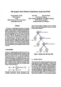
The vector w∗ ∈ Rn+1 is called a solution vector. Since the problem is linearly separable there are infinitely many solution vectors which belong to a region in Rn+1 formed by the intersection of the P positive half-spaces wT xi > 0 defined by the patterns xi , i = 1, · · · , P . Given the fact that all such hyperplanes intersect at the origin, the solution region has the shape of a hyper-cone, thus we’ll refer to it as the “solution cone”. In [11] an algorithm was developed for incrementally computing the solution cone Ck for the subset {x1 , · · · , xk }, given the solution cone Ck−1 for the subset {x1 , · · · , xk−1 }. Since Ck−1 is convex it can be defined by a set of edges ei so that any element of Ck−1 can be written as a convex combination of the edges and conversely, every convex combination of the edges is an element of Ck−1 , so, X w ∈ Ck−1 ⇔ w = ai ei , ai > 0.

negative edges

Fig. 1. The solution cone may need to be updated when a new pattern comes in. In general, the hyperplane associated with the new pattern xk generates sets of positive edges, negative edges, and new edges. The new edges are generated at the intersections of the incoming hyperplane and the existing cone facets. The positive and the new edges describe the new cone. is composed of all combinations of positive-negative edges and its cardinality is multiplicative with respect to the cardinalities of E+ and E− . If cp , cn , and cz is the number of positive, negative, and zero edges, respectively, then the new cone has cp +cp cn +cz edges as opposed to cp +cn +cz edges prior to the split. As a consequence, the algorithm is not very practical unless some garbage collection method is devised to discard redundant edges. In this case the method produces the minimal set of edges that defines the solution cone. Even so, the garbage collection algorithm can be very time consuming, especially for large data dimension n. Furthermore, the minimum set of edges, although smaller than the set of edges before garbage collection, may not be small in absolute size.

i

The new vector xk splits the cone separating the set of edges into positive, negative, and zero edges (see Fig. 1): E+ = {ei : i ∈ I+ }, I+ = {i : eTi xk > 0} E− = {ei : i ∈ I− }, I− = {i : eTi xk < 0} E0 = {ei : i ∈ I0 }, I0 = {i : eTi xk = 0}

new edge

(3) (4) (5)

According to the original algorithm the edges defining Ck are computed by the union of the following three sets: (a) the positive edges, E+ , (b) the zero edges, E0 , and (c) the new edges generated at the intersections of the incoming hyperplane and the existing cone facets, defined as [11]

3. UPDATING THE SOLUTION VECTOR The key observation that leads to the subsequent development of the proposed algorithm is that we do not actually want the edges but just a solution vector. In other words, we want to find some vector wk ∈ Ck given some wk−1 ∈ Ck−1 . Equivalently, given a positive linear combination of the edges for Ck−1 we want to obtain a positive linear combination for the edges of Ck . Any such vector wk−1 has the

Enew = {em = ej eTi xk − ei eTj xk : i ∈ I+ , j ∈ I− }. (6) Unfortunately, the number of edges grows very rapidly every time a new pattern splits the cone, since the set Enew

94

form wk−1

X

=

a i ei +

i∈I+

X

bj ej +

j∈I−

X

At the same time, since together the positive and the negative edges define the solution cone Ck−1 , we have eTi xj ≥ 0, for any i ∈ I− or i ∈ I+ , and j = 1, · · · , k − 1. For each i there are n indexes j1 , ..., jn such eTi xj1 = 0, ..., eTi xjn = 0, since ei is defined as the intersection of n hyperplanes. For the remaining k − 1 − n patterns xj we have eTi xj > 0. Thus for i = 1, · · · , k − 1,

cm em (7)

m∈I0

with ai , bj , cm > 0, while wk can be written as X X X wk = a0i ei + b0ij (ej eTi − ei eTj )xk i∈I+

X

+

i∈I+ j∈I−

c0m em

(8)

m∈I0

with a0i , b0ij , c0m > 0. Since the sizes of the edges are unspecified we may, without loss of generality, absorb all coefficients ai , bj , cm , a0i , b0ij , c0m , into the corresponding vectors to obtain simpler expressions as follows, X X X wk−1 = ei + ej + em (9) i∈I+

wk

=

X

ei +

i∈I+

+

j∈I−

X X

(ej eTi − ei eTj )xk (10)

m∈I0

Subtracting (9) from (10) we derive the following learning rule for updating wk−1 into wk wk = wk−1 + ∆wk

(11)

=

e+

=

(e− eT+ − e+ eT− )xk − e− X ei

> 0.

(18)

Assumption 1 The cumulative positive vector e+ is a positive sum of the previous solution vector wk−1 and the incoming pattern xk

where ∆wk

(17)

The learning rule (11) requires the updating of the solution vector every time a new pattern xk is presented, regardless whether this pattern is correctly classified by wk−1 or not. Let us simplify the learning process by taking wk = wk−1 T whenever wk−1 xk > 0. This is reasonable because our goal is to find a solution vector in the new cone Ck given wk−1 ∈ Ck−1 . In this case wk−1 ∈ Ck and so no update is necesT sary. Updating happens only when wk−1 xk < 0 using the learning rule (11), (12). This, however, requires the computation of the cumulative positive and negative edges e+ and e− . Using Eqs. (13), (14) is too costly. We would like to estimate e+ and e− without explicit computation of the individual positive and negative edges. This would result in massive computational savings. Motivated by the Perceptron algorithm let us work with the following assumption

m∈I0

em

> 0,

eT+ xi

3.1. Basic classification algorithm

i∈I+ j∈I−

X

eT− xi

(12)

e+ = awk−1 + bxk , 0 < a, b

(13)

(19)

i∈I+

e−

=

X

ei

(14) Let us make a further simplification by ignoring the zeroedges since they have zero probability

i∈I−

Observe that the updating term (12) involves the sum e+ of the positive edges and the sum e− of the negative edges, so the individual edges are not used. We shall call e+ and e− the cumulative positive edge and the cumulative negative edge, respectively. Furthermore, note that if the negative edge set is empty then e− = 0 and the update term ∆wk is zero. In other words, if the new hyperplane leaves the cone entirely on the positive side then no updating is required. On the other hand, if the cone lies entirely on the negative side of the new hyperplane then the problem is not linearly separable. By the definition of the cumulative positive and the negative edges we have eT− xk




0.

(16)

Assumption 2 The set E0 is empty. So by (9) we obtain wk−1 = e+ + e− .

(20)

e− = wk−1 − e+ = (1 − a)wk−1 − bxk

(21)

and

Substituting Eqs. (19), (21), in Eq. (12) we get ∆wk ∆wk

95

=

T bwk−1 kxk k2 − bxk wk−1 xk

=

−(1 − a)wk−1 + bxk [bkxk k2 − (1 − a)] wk−1 T −b[wk−1 xk − 1] xk

(22)

and T wk = [bkxk k2 + a]wk−1 + b[1 − wk−1 xk ]xk

Select an arbitrary positive value for a and a very small positive value for ε Initialize w using the first n patterns according to (30) for patterns k = n + 1, · · · , P let y = wT xk if (y < 0) set b to the value defined in (29) update w according to (23) normalize w end

(23)

For the learning rule (23) to be complete we must identify suitable values for the constants a and b. For this we take into account the constraints (15) and (16). Indeed, from Eq. (15) we get T (1 − a)wk−1 xk − bkxk k2 < 0

(24)

T b > (1 − a)wk−1 xk /kxk k2

(25)

and similarly, from Eq. (16) T awk−1 xk

b>

Fig. 2. Algorithm 1: basic learning rule. 2

+ bkxk k > 0

T −awk−1 xk /kxk k2

(26) The update formula (23) imposes an unspecified scaling on the norm of wk . For stability reasons the vector needs to be normalized after each update. Fig. 2 summarizes the proposed algorithm. Note that b in (29) is a function of a which is an arbitrary positive number. In order to study the significance of a let us substitute (29) in (23) to get

(27)

T Combining (25) and (27) with the fact that wk−1 xk < 0, we obtain T n o −wT x |wk−1 xk | k−1 k b > max (a − 1), a = a 2 kxk k kxk k2

(28)

wk

There is an additional set of 2(k −1) constraints coming from Eqs. (17), and (18), but their satisfaction using just two parameters, a and b, is obviously an overdetermined problem. Additionally, there is a computational cost associated with checking these constraints and, to make things worse, this cost increases with the number of patterns k. We avoid the problem altogether by making the simplifying assumption that if the value of b is “barely” above the lower bound described by (28) then very few older patterns will be violated since the new vector wk gets “barely” inside the new cone. Therefore we let b=a

T |wk−1 xk | +ε kxk k2

T [−awk−1 xk + εkxk k2 + a]wk−1 T T −awk−1 xk /kxk k2 [1 − wk−1 xk ]xk

wk

=

T +ε[1 − wk−1 xk ]xk h i T a[1 − wk−1 xk ] I − xk xTk /kxk k2 wk−1 h i +ε xk + [kxk k2 I − xk xTk ]wk−1 (31)

Using the projector operator Pk = I − kx1k k2 xk xTk for the subspace orthogonal to xk , (31) can be simplified into h ε ε i T wk = a (1 − wk−1 xk + kxk k2 ) Pk wk−1 + xk (32) a a Since wk is normalized at each iteration, the pre-multiplication of (32) by a is insignificant. The only effect carried by a is the scaling of ε, which is an arbitrary constant, anyway. Therefore, the value of a is practically inconsequential. We may use any positive number that will simplify our computations, for example, a = 1.

(29)

where ε is a very small positive number. 3.1.1. Initialization, normalization and the parameter a The algorithm needs a starting vector wP0 which must belong to the solution cone CP0 of some patterns xi , i = 1, · · · , P0 . It is easy to produce such a starting point (call it wn ) for the first n patterns by solving the following system of equations

3.2. Improving the basic algorithm The basic algorithm presented in Fig. 2 has the drawback that it may fail to separate a linearly separable problem. Although our simulations show that in the linearly separable scenario the misclassified patterns, after training with Algorithm 1, are a very small fraction of the total patterns, this performance is not acceptable. A simple modification that considerably improves the performance is to use training epochs, ie. to repeatedly sweep the data with Algorithm 1,

xTi wn = 1, i = 1, · · · n so wn = [x1 , · · · , xn ]−T [1, · · · , 1]T

=

(30)

96

so that in each epoch the initial vector is the final vector of the previous epoch. 4. EXPERIMENTS: NAMED ENTITIES RECOGNITION Named Entities Recognition (NER) is the task of recognizing and classifying phrases within a document that belong into the following categories: person (PER), location (LOC), organization (ORG), and miscellaneous (MISC) for example, book or film titles. This task is very useful for creating semantic representation of sentences like in the case of Information Extraction systems [13] and Human-Machine Dialogue systems, or simply for indexing texts [14]. See related conferences-competitions of NER systems [15, 12]. The experiment described herein concerns Greek NER. For each Named Entity (NE) we annotate the beginning token, marked [B-X], and the inside tokens (if any), marked [I-X], where X=PER, ORG, LOC, or MISC. Non NE’s are marked [O]. An example (in English) would be the following: ”Wolff [B-PER] ,[O] currently[O] a[O] journalist[O] in[O] Argentina[B-LOC] ,[O] played[O] with[O] Del[B-PER] Bosque[I-PER] in[O] Real[B-ORG] Madrid[I-ORG] .[O]” 4.1. The Corpus The corpus we used is a selection of 400 articles of the year 1997 of the Greek newspaper ”TA NEA” covering diverse thematic fields. The corpus measures approximately 172.000 tokens. We have divided the corpus into two parts. The training part (approximately 138.000 tokens) and the testing part (approximately 34.000 tokens). We used the tools provided with the Ellogon Text Engineering Platform [16] in order to: (a) split the two corpora into sentences and tokens (use of a Sentence Splitter and a Tokeniser) (b) obtain Part of Speech (PoS) tags for all tokens of the two corpora (use of the Greek version of Brill’s PoS Tagger [17]) (c) manually annotate the NE in the two corpora, and (d) construct the inputs of the features extraction tool for both training and testing corpora.

information related to the current token or its close context. Local features concern the current token, the previous one, the previous two, the next one, and the next two tokens. Local features use morphological and word-lists information. Morphological information gives features such as the following: “Does current token begin with a capital letter?”, “Is current token the first token of a sentence?”, or “Has previous token a noun PoS tag?”, etc. Word lists (for example, list of Greek person names, etc) present important information that can be used to form features such as the following: ”Is current token a member of a person names list?”, ”Is current token a part of a list of tokens tagged in the training corpus as I-LOC?”, or ”Does current token end with one of the suffixes contained in the Greek person names suffixes list?”, etc. 4.3. Experimental Results We have used our training and test data to compare our method (named “ONETIME”) against two state of the art classifiers (1) Support Vector Machines using the SVMlight freeware [19] and (2) Maximum Entropy Models [20, 21] implemented by the freeware “MaxEnt toolkit” [22]. All these methods are binary classifiers. Since our problem is a nine-class problem we transformed it into 36 binary problems using all pairs of classes (also known as the ”Round Robin” approach [23]). In order to decide whether a pattern belongs to a certain class we use voting to combine the classifier decisions for this class against the other eight classes. NER systems are evaluated using the precision, recall and F-measure scores. The precision of a system is the percentage of correctly classified NE tokens among all the tokens classified as NE by the system. The recall of a system is the percentage of correctly classified NE tokens compared to the NE tokens assigned manually in the test corpus. The F-measure is a combination of precision and recall calculated by the following formula: Fβ =

4.2. Feature Selection

(β 2 + 1) ∗ precision ∗ recall (β 2 ∗ precision + recall)

(33)

We experimented with different values of ε in (29) and the results presented here correspond to ε = 0.006. The best scores achieved with all three methods can be seen in Table 1. Comparing the overall F-Measures of the three methods we can see that our method has very competitive scores with Maximum Entropy (87.05 vs 87.19) as well as with linear SVMs (87.05 vs 87.40). In some classes, for instance, the ORG class our method outperforms both the Maxent and the Linear SVM methods. Furthermore, in the MISC class the overall F-measure outperforms the Maxent. These results are very promising since the method has not yet been fine tuned. Possible lines of improvement include the selection

The features we used for both training and evaluating the systems where mainly inspired by Chieu and Ng [18]. The features are all binary, and there are two types of features: global and local. Global features make use of information within the whole article (the corpus is divided in several articles): for example, if the current token is made up of all capitalized letters and its size is greater than 2 characters we look in the same article for sequences of initial capitalized tokens where the sequence of their initial letters matches the current token. If found, this feature is set to 1 (this feature helps recognizing acronyms). Local features make use of

97

Method Maxent SVM (P) SVM (L) Onetime Method Maxent SVM (P) SVM (L) Onetime Method Maxent SVM (P) SVM (L) Onetime

PERSON R Fβ=1 95.25 95.90 96.61 96.53 96.18 95.94 94.90 95.10 ORG P R Fβ=1 83.93 76.15 79.85 85.76 79.32 82.42 83.84 74.29 78.78 85.05 76.41 80.50 OVERALL P R Fβ=1 91.99 82.86 87.19 92.46 85.36 88.77 91.39 83.75 87.40 91.25 83.22 87.05 P 96.57 96.46 95.70 95.31

P 90.04 89.56 88.71 88.18 P 88.80 90.57 88.90 89.40

LOC R 87.57 89.30 88.58 88.44 MISC R 55.69 60.83 59.44 57.57

Fβ=1 88.79 89.43 88.64 88.31 Fβ=1 68.45 72.78 71.25 70.04

[9] E. Osuna, R. Freund, and F. Girosi, “An Improved Training Algorithm for Support Vector Machines,” in Proc. IEEE Neural Networks for Signal Processing VII Workshop, Piscataway, N.J., 1997, pp. 276–285, IEEE Press. [10] B. E. Boser, I. M. Guyon, and V. N. Vapnik, “A Training Algorithm for Optimal Margin Classifiers,” in Proc. Fifth Ann. Workshop Computational Learning Theory, New York, 1992, pp. 144–152, ACM Press. [11] K. I. Diamantaras and M. G. Strintzis, “Neural Classifiers Using One-Time Updating,” IEEE Trans. Neural Networks, vol. 9, no. 3, pp. 436–447, May 1998. [12] E. F. Tjong Kim Sang, “Introduction to the CoNLL-2002 Shared Task: Language-Independent Named Entity Recognition,” in Proceedings of CoNLL-2002, Taipei, Taiwan, 2002, pp. 155–158. [13] N. Chinchor, “MUC-7 Information Extraction Task Definition (version 5.1),” in Proceedings of 7th Message Understanding Conference, Fairfax, VA, 19 April - 1 May 1998.

Table 1. The Precision (P), Recall (R), and F-measure (F) for the NER task using 4 classification schemes: the Maximum Entropy method (Maxent), SVM with polynomial or linear kernels (SVM-P or SVM-L) and our method (Onetime).

[14] N. Friburger and D. Maurel, “Textual Similarity Based on Proper Names,” in Proceedings of the workshop Mathematical / Formal Methods in Information retrieval (MFIR ’2002) at the 25th ACM SIGIR Conference, Tampere, Finland, 2002, pp. 155–167. [15] N. Chinchor, “MUC-7 Named Entity Task Definition (version 3.5),” in Proceedings of 7th Message Understanding Conference, Fairfax, VA, 19 April - 1 May 1998.

of the optimum order of the training patterns as well as the selection of the optimal value of ε. These factors seem to play a significant role in improving the results.

[16] G. Petasis, V. Karkaletsis, G. Paliouras, I. Androutsopoulos, and C. D. Spyropoulos, “Ellogon: A New Text Engineering Platform,” in Proceedings of the 3rd International Conference on Language Resources and Evaluation (LREC-2002), Las Palmas, Canary Islands, Spain, May 2002, pp. 72–78.

5. REFERENCES [1] F. Rosenblatt, “The perceptron: A probabilistic model for information storage and organization in the brain,” Psychological Review, vol. 65, no. 6, pp. 386–408, 1958.

[17] E. Brill, “A simple rule-based part-of-speech tagger,” in Proceedings of ANLP-92, 3rd Conference on Applied Natural Language Processing, Trento, Italy, 1992, pp. 152–155.

[2] B. Widrow and F. W. Smith, “Pattern-recognizing control systems,” in Computer and Information Sciences (COINS) Proceedings, Washington, D.C., 1964.

[18] H. L. Chieu and H. T. Ng, “Named Entity Recognition with a Maximum Entropy Approach,” in In Proceedings of CoNLL2003, Edmonton, Canada, 2003, pp. 160–163.

[3] Y.-C. Ho and R. L. Kashyap, “An algorithm for linear inequalities and its applications,” IEEE Trans. Elec. Comp., vol. 14, pp. 683–688, 1965.

[19] Thorsten Joachims, http://svmlight.joachims.org/.

[4] V. Vapnik, The Nature of Statistical Learning Theory, Springer-Verlag, New York, 1995. [5] S. Theodoridis and K. Koutroubas, Academic Press, 1998.

ing, B. Sch¨olkopf, C. Burges, and A. Smola, Eds., pp. 169– 184. MIT Press, Cambridge, MA, 1999.

“SVMlight

software,”

[20] A. L. Berger, V. J. Della Pietra, and S. A. Della Pietra, “A Maximum Entropy Approach to Natural Language Processing,” Computational Linguistics, vol. 22, no. 1, pp. 39–71, 1996.

Pattern Recognition,

[21] A. Borthwick, A Maximum Entropy Approach to Named Entity Recognition, Ph.D. thesis, New York University, Department of Computer Science, Courant Institute, 1999.

[6] R. O. Duda, P. E. Hart, and D. G. Stork, Pattern Classification, Wiley Interscience, 2nd edition, 2000. [7] J. C. Platt, “Fast Training of SVMs Using Sequential Minimal Optimization,” in Advances in Kernel Methods Support Vector Learning, B. Sch¨olkopf, C. Burges, and A. Smola, Eds., pp. 185–208. MIT Press, Cambridge, MA, 1999.

[22] Zhang Le, “Maximum Entropy toolkit,” http://homepages.inf.ed.ac.uk/s0450736/maxent toolkit.html. [23] J. Fuernkranz, “Round Robin Classification,” The Journal of Machine Learning Research, vol. 2, pp. 721–747, March 2002.

[8] T. Joachims, “Making Large-Scale SVM Learning Practical,” in Advances in Kernel Methods Support Vector Learn-

98