Center for Computational Statistics and Probability, Fairfax, VA 22030. 1. .... graphics are clear well-known examples of what we call computational statistics.
A VIEW OF COMPUTATIONAL STATISTICS AND ITS CURRICULUM Edward J. Wegman, George Mason University Center for Computational Statistics and Probability, Fairfax, VA 22030 1. Introduction. The spectacular growth in the field of computing science is obvious to all. Indeed, the most obvious manifestations, the ubiquitous microcomputer, is in some ways perhaps the least significant aspect of this revolution. The new pipeline and parallel architectures including systolic arrays and hypercubes, the emergence of artificial intelligence, the cheap availablility of RAM and color graphics, the impact of high resolution graphics, the potential for optical, biological and chemical computing machines and the pressing need for software/language models for parallel computing are all aspects of the computation revolution which figure prominently in the other sciences. While not as obvious to the casual observer, the fields of statistics and probability have experienced equally spectacular technical achievements including weak convergence theory, the almost sure invariance principle, exploratory data analysis, nonlinear time series methods, bootstrapping, semiparametric methods, percolation theory, simulated annealing and the like principally within the last decade. The computing and statistical technologies both figure prominently in the manipulation and analysis of data and information. It is natural then to consider the linkage between these two discipline areas. The interface between these two discipline areas has been labeled by the phrase, “statistical computing," and more recently, “computational statistics." We should like to distinguish between the two and, indeed, argue that the latter embodies a rather significantly different approach to statistical inference. In thinking carefully about the relationship between computing science and statistical science it is possible to describe a large number of linkages. Two that come immediately to mind are the stochastic description of data flow through a computer and the characterization of uncertainty in expert systems. In the former case, we can view a computing architecture, particularly a parallel or distributed architecture as a network with messages being passed from node to node. This is essentially a queueing network and the characterization of the distribution state of the network becomes a problem in stochastic model building and estimation. In the latter example, a rule-based expert system is invariably characterized by imprecision in the specification of the basic predicates derived from the expert or experts. This may be because either the rule is a “rule-of-thumb" and hence inherently imprecise or because the rule is a not yet fully formulated and verified inference and hence exogenously stochastic. The assignment of probabilities (or such alternatives to probabilities as belief functions or fuzzy set functions) in a useful way is another application of statistical methodologies to computing science. In both of these examples statistical methodology is employed in the development of computing
science. Both of these examples might legitimately be called statistical computing since the focus is on computing with statistics as an adjectival modifier. Traditionally, of course, this is not at all what statistical computing means. Statistics is fundamentally an applied science, hence, a computationally oriented science. A statistical theory is useless without a suitable algorithm to go with it. Statistical computing has traditionally meant the conversion of statistical algorithms into a reasonably friendly computer code. This enterprise became feasible with the development of the IBM 360 series in the early 1960s and the slightly later development of the DEC Vax series of computers. Of course, the trend has accelerated with the ubiquitous PC. Packages such as SAS, BMDP, Minitab, SPSS and the like represent a very high evolution in statistical computing. When we use the phrase, “computational statistics," we have in mind a rather stronger focus on the exploitation of computing in the creation of new statistical methodology. We shall give some explicit examples shortly. 2. Statistics as an Information Technology. Statistics is fundamentally about the transformation of raw data into useful information. As such statistics is a fundamental information technology. It is, therefore, appropriate to see statistical science as intimately related not only to computing science, but also communication technology, electrical engineering and systems engineering as part of the spectrum of modern information processing and handling technologies. Statistics is perhaps the oldest and most theoretically well developed of these information technologies. It is thus important to understand how the changing face of these technologies affect statistics and, more importantly, how they offer new opportunity for the development of statistical methodologies. In particular, it is important to understand how the computer revolution is affecting the accumulation of data. Electronic instrumentation implies an ability to acquire a large amount of high dimensional data very rapidly. While such capabilities have existed for some time, the emergence of cheap RAM in the 1980's has given us the ability to store and access that data in an active computer memory. Satellite-based remote sensing, weather and pollution monitoring, data base transactions, computer controlled industrial automation and computer controlled laboratory instrumentation as well as computer simulations are all sources of such complex data sets. We contend that this new class of data represents a challenge for statisticians which is substantially different in kind. In many ways the characteristics of automated data are different from traditional data. Automated data is generally untouched by human brain. While there are fewer transcription errors, there are also fewer checks for reasonableness. There are likewise different economic considerations. In many traditional data collection regimes, the cost per item of data is expensive. In the automated mode, set-up costs are expensive, but once accomplished there is low incremental cost for taking additional data. Thus it is often easy to replicate, hence, increased sample size, and it is easy to to take additional measurement on each sample item (variables), hence an increase in dimensionality. As an adjunct, it is worth pointing out that when an individual datum is expensive, we collect no more than absolutely needed to complete the inference.
However, when the marginal cost of additional data is low, we tend to collect much more both in sample size and dimension motivated by the belief that it might be useful for some not-yetprecisely-specified purpose. Thus, the computing revolution often implies that there are less sharply focused reasons for collecting data. The majority of existing methodology is focused on the univariate, IID random variable model. Even in the circumstance that a multivariate model is entertained, it is usually assumed to be multivariate normal. We contend, in addition, that while arbitrary sample size is frequently assumed, the truth of the matter is that these techniques implicitly assume small to moderate sample sizes. For example, a regression problem with 5 design variables and 1000 observations would represent no problem for traditional techniques. By contrast, a regression problem with 40,000 design variables and 8 million observations would. The reason is clear. In the former case the emphasis is on statistical efficiency which is the operational goal for most current statistical technology. However, with massive replications the need for statistical efficiency is much less pervasive. Indeed, we may find it desireable to exchange highly efficient, parametric procedures for less efficient, but more robust, nonparametric procedures to guard against violations of (possibly untestable) model assumptions. The emphasis on parsimony in many contemporary books and papers is a further reflection of the mind-set that implicitly focuses on small to moderate sample sizes since few parameters do not necessaily make sense in the context of very large sample sizes. Finally, we note that the very fact of largeness in sample size implies that it is unlikely we would see IID homogeneity. Thus, the computer revolution implies a revolution in the type of data we are able to accumulate, i.e. large, high-dimensional nonhomogeneous data sets. More importantly, however, the richness of these new data structures suggest that we are more demanding of the data. In a simple univariate IID setting we primarily are concerned with variability of a single random variable and questions related to this variability. In a more complex data set, however, it is natural to ask more involved questions while simultaneously having less a priori insight into the structure of the data. When more variables are available, we would certainly ask about the functional relationship among them. We have used the phrase, structural inference, for methodologies aimed at describing such relationships, deliberately contrasting this phrase with the phrase, statistical inference, which has traditionally been about determining variability (i.e. probability distributions). With a more complex structure, we are open to ask more of the data than just simple decisions. We may want to ask forecasting questions, e.g. about weather, economic projections, medical diagnosis, university admissions and tax audits, or questions about automated pattern recognition, e.g. printed or hand-written characters, speech recognition and robotic vision, or questions about system optimization, e.g., process and quality control, drug effectiveness, chemical yields and physical design. The contrast between traditional statistics and the new statistics is marked and strong. We summarize in Table 1. We think that the implications of the computer revolution on statistics are sufficient to warrant new terminology, specifically computational statistics. This terminology not only provides the linkage of statistical science with computing science, but also puts the focus on statistics rather than on computing.
3. Some Examples. In this section we should like to illustrate these notions of computational statistics with three examples of approaches to data that flow from thinking about statistics in light of contemporary computation. TRADITIONAL STATISTICS Small to Moderate Sample Size IID Data Sets One or Low Dimensional Manually Computational Mathematically Tractable Well Focused Questions Strong Unverifiable Assumptions relationships (linearity,additivity) error structures (normality) Statistical Inference Predominantly Closed Form Algorithms Statistical Optimality
COMPUTATIONAL STATISTICS Large to Very Large Sample Size Nonhomogeneous Data Sets High Dimensional Computationally Intensive Numerically Tractable Imprecise Questions Weak or No Assumptions relationships (nonlinearity) error structures (distrib. free) Structural Inference Iterative Algorithms Possible Statistical Robustness
Table 1. Comparsion of Traditional and Computational Statistics It goes without saying that such techniques as bootstrapping, cross validation and high interaction graphics are clear well-known examples of what we call computational statistics. We wish to describe two less well known ideas: 1. functional inference and 2. data set mapping. 3.1 Example: Functional Inference. Our fundamental premise is that we are interested in the structural relationship among a set of random variates. We formulate this as follows. Given the random variables X� , X� , Ã , X� which are functionally related by an equation, f(X� ,Ã ,X� ) ~ �, determine f. This is a generalization of the problem of finding the prediction equation in the standard regression problem, Y c x� ~ �, but in a nonparametric, nonlinear setting. We suggest the following notion. Let M ~ ¸(x� ,Ã ,x� ): Ef(x� ,Ã ,x� ) ~ 0¹. M in general is an algebraic variety and under reasonable regularity conditions a manifold. Thus, there is a fundamental equivalency between estimating the geometric manifold M and estimating the function f. By turning our attention to the manifold M, we make the problem a geometric one, one whose structure is easier to visualize using computer graphics. For this reason we believe there is an intimate connection between the structural estimation problem and the visualization of high dimensional manifolds. While graphical methods for looking at point clouds have proven stimulating to the imagination, it is extremely difficult to understand true hyperdimensional structure, particularly when rotating about an invisible axis. We believe that a solid structure as
opposed to a point cloud would provide the visual continuity to alleviate much of this problem. This solid structure is what we identify with the manifold M. To get a handle on the procedure for estimating a manifold we note a d-ridge is the extremal d-dimensional feature on a hyperspace structure of dimension greater than d. The 0-ridge corresponds to the usual mode. For some d, we contend that a reasonable estimate of M is the d-ridge of the n-dimensional density function of (X� , Ã ,X� ). This in effect is estimating the d-dimensional summary manifold with a mode-like estimator. In essence what we are suggesting to skeletonize hyperdimensional structures. This type of process has been done in the image processing context with good computational efficiency. The inference technique then is to estimate M nonparametrically. This reduces the scatter diagram to a geometrically described hyperdimensional solid. This can then be explored geometrically using computer graphics. Features can then be parametrized and a composite parametric model constructed. The inference can be completed by a confirmatory analysis on the (perhaps nonlinear) parametric model. Techniques presently in use often assume linearity or special forms of nonlinearity, e.g. polynomial or spline fits, and often assume additivity a low dimensional subcomponents, e.g. projection pursuit. We would not like to take this perspective a priori. While this methodology may consequently seem complex, the premise is that geometric-based structural analysis will offer tools superior to traditional purely analytic methods for building high dimensional functional models. The key to this development is to appreciate the role of ridges in describing relationships between random variables. A simple two-dimensional example is illustrated in Figure 3.1. Note that the contours represent the density and the 1-ridge represents the functional relationship between x and y in a traditional linear regression. Since densities are key, a fast, efficient multidimensional density estimation technique is important. The slowness of the traditional kernel estimators in a high dimensional setting arises from the fact that they are essentially point estimators. That is to say, to compute f(x) one needs to do smoothing in a neighborhood of x. For a satisfying visual representation, the x's must be chosen reasonably dense. Moreover, traditional kernels are frequently nonlinear functions and thus the computation involves the repeated evaluation of a nonlinear function at each of the observations of a potentially large data set on a dense set of points in the domain. Furthermore, as dimension increases, exponentially more domain points are required to maintain a constant number of points per unit hypervolume. Traditional kernel estimators become essentially useless for even relatively low dimensions. The traditional histogram provides an alternative strategy. The histogram is a two-step procedure. The first step is a tesselation of the line. The second step is an assignment of each observation to a tile of that tesselation. The computation of the actual density estimator amounts to a simple rescaling of tile- (cell-) count. The histogram is a global estimator since the function is constant on the tiles which are finite in number and, indeed, relatively few in number compared with the denseness of points required required for the kernel estimator. The traditional histogram, of course, operates with fixed equally spaced uniform tiles. There is no reason why the tiles must be fixed or uniform. Wegman (1975) suggests a data- dependent
tesselation in the one dimensional setting and shows that, if the number of tiles is allowed to grow at an appropriate rate with the increase of sample size, then asymptotic consistency can be achieved. The ingenious papers by Scott (1985, 1986) introduce the notion of the average shifted histogram, ASH. Scott recognizes the computational speed of a global estimator such as the histogram. His algorithm computes the histogram for a variety of tesselations and then averages these together to obtain smoothing properties. In this paper we are suggesting a combination of these two ideas. We propose a data-driven tesselation of the following sort. Take an �% (10%) subsample of the sample. Use these points to form a Dirichlet tesselation of n-space. A two dimensional example is given in Figure 3.2. The tiles of the Dirichlet tesselation form the datadependent convex regions upon which to base the density estimator. One pass through the data will be sufficient to classify each point according to tile and thence a simple rescaling to compute the estimator. Repeated subsampling will yield additional estimators which can then be averaged in the manner of Scott's ASH. The details of this algorithm need to are being explored, but the following conjectures are made. Asymptotic properties similar to those found in Wegman (1975) hold. Maximum likelihood and nearest neighbor properties will hold. Computational efficiency will be substantially better than with kernel methods. Because of the repeated sampling, bootstrap-type behavior will hold. It should be clear that the notions we are suggesting rely heavily on the generalization of present geometric algorithms to higher dimensional space. The Dirichlet tesselation, for example, has useful algorithms in 2 and 3 dimensions (see Bowyer, 1981, Green and Gibson, 1978), but the analogues in higher dimensions are poorly developed (see Preparata and Shamos, 1986). Thus a fundamental exploration of algorithms for these tesselations in hyperspace must still be done. Interestingly enough, the computation of tesselations in hyperspace is closely related to the computation of convex hulls (again see Preparata and Shamos, 1986, p. 246). The construction of the n-dimensional Dirichlet tesselation (Voronoi diagram) is a key element of the density estimation technique we suggest. A related issue is the assignment problem, that is, given the tiles, what is the best algorithm for determining to which of the tiles a given observation belongs. In part the 2-dimensional Voronoi diagrams were constructed to answer nearest-neighbor-type questions. That is, given n points, what is the best algorithm (minimum compute time) for finding the nearest neighbor. In general, the answer is known to be O(nd) where d is the dimension of the space. There is some reasonable expectation that, since the construction of the tesselation and the assignment problem are closely linked, there is an efficient one-step algorithm for sorting the observations in convex regions about certain nearest neighbors. If this could be done in linear, near linear or even polynomial time, the density estimation technique we are suggesting may be computationally feasible for relatively high-dimensional cases. In any case, the sorting, clustering and classification results which form the core of computational geometry also form the core of this approach to higher dimensional data structures.
We hope that this example makes clear the mathematical complexity inherent in computational statistics. It is our view that there is an extremely important role for mathematical statistics under the general rubric of computational statistics. 3.2 Example: Data Set Mapping. A traditional way of thinking about the model building process is that we begin with a fixed data set and apply a number of exploratory procedures to it in search of structure within the data set. The data set is regarded as fixed and the analysis procedures as variable. Of course, the model is iteratively refined by checking the residual structure until a suitable model reduces the residuals to a unstructured set of “random numbers." We suggest an alternative way of thinking. Normal Mode of Analysis: Data Set Fixed ¥ Try Different Techniques on It Alternative Mode of Analysis: Techniques Set Fixed ¥ Try Different Data on It We have in mind the following. With the cost or availablility of computational resources essentially not a significant consideration in the analysis procedure (i.e. they are essentially a free good), we can afford to standardize on say a dozen or more techniques which are always computed no matter what data are presented. Others, of course, would still be optionally available. Such standard techniques might include for example standard descriptive statistics, smoothers, spectral estimators, probability density estimators and graphical displays including 3-D projections, scatter diagram matrices, parallel coordinate plots, grand tours, Q-Q plots, variable aspect ratio plots and so on. Each of these might be implemented on a different node of a parallel computing device and displayed in a window of a high resolution graphics workstation, analogous to having a set of papers on our desk through which we might shuffle at will, the difference being that each sheet of paper would, in effect, contain a dynamic, possibly multidimensional display with which the analyst might interact. We have in mind viewing each of these data representations as an attribute of the data set (object orientation) so that if we modify the data set representation in one window, the fundamental data set is modified and consequently its representations in all of the windows are modified simultaneously. With the set of techniques fixed, a data analysis proceeds through an iterative mapping of the data set, i.e. the data set is iteratively re-expressed. This is done by a series of techniques. A discriminant procedure or a graphical brushing procedure allows us to transform one data set into a number of more homogeneous data subsets. Data transformations, rescaling either linear or nonlinear, clustering, removing outliers, transforming to ranks, bootstrapping, spline fitting and model building are all techniques for mapping an old data set into one or more new ones. Notice that we treat modeling building as a simple data map. It is our perspective that a model fit is just a transformation of one data set to another (specifically the residuals) similar to any of the others mentioned.
Two points of interest can be made. First, the analysis of a data set can be viewed as the development of a data tree structure - each node is a data set and each edge is a transformation or re-expression of that data set to a new data set. The data tree structure preserves the record of the data analysis, indeed, the data tree is the data analysis. At the bottom of the data tree presumably we will have data sets with no remaining structure for, if not, then another iteration of our analysis and another edge in the data tree are required. The second point to be made is that thinking in the terms just described helps clarify our thinking by conceptually separating the representational methods (e.g. graphics, desciptive statistics) from the re-expression methods (transformations, brushing, outlier removal, model building). These are really two separate functions of our statistical methodology which are not commonly distinguished, but when distinguished, aid in clearer thinking. We particularly think it is helpful to understand, for example, that a square-root data transformation and a ARMA-model fitting are really quite similar operations each resulting in a new data set save that in the latter case we usually call the new data set the set of residuals. Indeed, when the data analysis is completely laid out as a data tree, the full model is really accumulated by starting at the root node (original data set) and following the edges all the way to the ending node (unstructure residual data set).
4. Curriculum Implications. First of all, it is important to recognize that operating from the perspective of computational statistics does not imply that traditional statistical methodologies are obsolete. While some automated data sets will have the characteristics described earlier, many will not. In addition there will, no doubt, continue to be many carefully designed experiments in which each data point is costly to acquire, and, hence, traditional methods will continue to be used. Nowhere is this probably more true than in the case of biomedical clinical trials. We believe there are certain shifts in emphasis, however, that may be useful to recognize. In terms of mathematical preparation, real and complex analysis and measure theory are frequently emphasized as elements of a graduate curriculum. These are tied to probability theory and the more-or-less standard IID parametric assumptions. To the extent that the questions we ask of data are less structured, much of the need for the standard frameworks and probability models is lessened. In their place we will tend to have a more geometric analysis and a more function-oriented, nonparametric framework. The first and second examples were deliberately chosen to illustrate elements of projective geometry, differential geometry and computational geometry. In addition, there is a strong element of nonparametric functional inference in Example 3.1 suggesting a heavier reliance on functional analysis. We believe therefore that functional analysis and geometric analysis should become part of the mathematical precursors to a statistics curriculum. That computation will play a role is obvious, exactly what form it will take is not so obvious. Certain elements of computing science would appear to be candidates. Computational literacy means more than FORTRAN or C programming or familiarity with the statistical
packages. Clearly such concepts as object-oriented programming, parallel architectures, computer graphics and numerical methods will play a significant role in future curricula. In terms of the statistical core material itself, I believe the obsession with the parametric framework (be it classical or Bayesian) must end. It is important to recognize that we are often dealing opportunistically collected data and that classical formulations are too rigid. Moreover, as indicated earlier, we are asking more of our data than simply distributional questions. Indeed the more interesting questions are the structural questions (i.e., in the face of unceratinty, how are two or more random variables related to each other?). Thus, it would seem that there should be some de-emphasis of traditional mathematical statistics (testing and estimation) and more emphasis on exploratory and structural inference. A contrast between a traditional first year curriculum and a revised curriculum is laid out in Figure 4.1 Acknowledgements. This paper has benefitted from several conversations with Jerry Friedman. I would like to thank him not only these discussions, but also his enthusiasm for the computational statistics. This research was supported by the Air Force Office of Scientific Research under Grant AFOSR-87-0179 and by the Army Research Office under Grant DAAL03-87-G-0070. REFERENCES Bowyer, A. (1981), “Computing Dirichlet Tesselations," Computer J. 24, 164-166. Green, P. J. and Gonson, R. (1978), “Computing Dirichlet Tesselations in the Plane," Computer J. 21, 168-173. Inselberg, A. (1985), “The Plane with Parallel Coordinates," The Visual Computer 1, 69-91. Preparata, F. P. and Shamos, M. L. (1986), Computational Geometry: An Introduction, New York: Springer-Verlag, Inc. Scott, D. W. (1985), “Average Shifted Histograms: Effective Nonparametric Density Estimators in Several Dimensions," Ann. Statist. 13, 1024-1040. Scott, D. W. (1986), “Data Analysis in 3 and 4 dimensions with Nonparametric Density Estimation," in Statistical Image Processing and Graphics, (Wegman, E and DePriest, D. eds.) New York: Marcel Dekker, Inc. Wegman, E. J. (1975), “Maximum Likelihood Estimation of a Probability Density, Sankhya (A) 37, 211-224. Wegman, E. J. (1986), “Hyperdimensional Data Analysis Using Parallel Coordinates," Technical Report 1, Center for Computational Statistics and Probability, George Mason University, Fairfax, VA, July, 1986.