Nonlin. Processes Geophys. Discuss., https://doi.org/10.5194/npg-2017-19 Manuscript under review for journal Nonlin. Processes Geophys. Discussion started: 12 June 2017 c Author(s) 2017. CC BY 3.0 License.
Multi-scale event synchronization analysis for unravelling climate processes: A wavelet-based approach Ankit Agarwal1, 2, 3, Norbert Marwan2, Maheswaran Rathinasamy4, Bruno Merz1, 3, Jürgen Kurths1, 2 5
1
University of Potsdam, Institute of Earth and Environmental Science, Karl-Liebknecht-Strasse 24-25, 14476 Potsdam, Germany 2 Potsdam Institute for Climate Impact Research, P.O. Box 60 12 03, 14412 Potsdam, Germany 3 GFZ German Research Centre for Geosciences, Section 5.4: Hydrology, Telegrafenberg, Potsdam, Germany 4 MVGR College of Engineering, Vizianagaram, India
10 Correspondence to: A. Agarwal (
[email protected]) Abstract. The temporal dynamics of climate processes are spread across different time scales and, as such, the study of these processes only at one selected time scale might not reveal the complete mechanisms and interactions within and between the (sub-) processes. For capturing the nonlinear interactions between climatic events, the method of event synchronization has 15
found increasing attention recently. The main drawback with the present estimation of event synchronization is its restriction to analyse the time series at one reference time scale only. The study of event synchronization at multiple scales would be of great interest to comprehend the dynamics of the investigated climate processes. In this paper, wavelet based multi-scale event synchronization (MSES) method is proposed by combining the wavelet transform and event synchronization. Wavelets are used extensively to comprehend multi-scale processes and the dynamics of processes across various time scales. The proposed
20
method allows the study of spatio-temporal patterns across different time scales. The method is tested on synthetic and realworld time series in order to check its replicability and applicability. The results indicate that MSES is able to capture relationships that exist between processes at different time scales. Keywords: multi-scale, event synchronization, discrete wavelet transformation, significance test
1 Introduction 25
Synchronization is a wide-spread phenomenon that can be observed in numerous climate-related processes, such as synchronized climate changes of the north and south Polar Regions (Rial 2012), see-saw relationship between monsoon systems (Eroglu et al., 2016), or coherent fluctuations in flood activity across regions (Schmocker-Fackel and Naef 2010) and among El Niño and the Indian summer monsoon (Marun and Kurths 2005; Mokhov et al., 2011). Synchronous occurrences of climate-related events can be of great societal relevance. The occurrence of strong precipitation or extreme runoff, for instance,
30
at many locations within a short time period may overtax the disaster management capabilities. 1
Nonlin. Processes Geophys. Discuss., https://doi.org/10.5194/npg-2017-19 Manuscript under review for journal Nonlin. Processes Geophys. Discussion started: 12 June 2017 c Author(s) 2017. CC BY 3.0 License.
Various methods for studying synchronization are available, based on recurrences (Marwan et al., 2007; Donner et al., 2010; Arnhold et al., 1999; Le Van Quyen et al., 1999; Quiroga et al., 2000; Quiroga et al., 2002; Schiff et al., 1996), phase differences (Schiff et al., 1996, Rosenblum et al., 1997), or the quasi-simultaneous appearance of events [Tass et al., 1998; Stolbova et al., 2014; Malik et al., 2012; Rheinwalt et al., 2016). For the latter, the method of event synchronization (ES) has received 5
popularity owing to its simplicity, in particular within the fields of brain [Pfurtscheller and Silva 1999; Krause et al., 1996) and cardiovascular research (O’Connor et al., 2013), non-linear chaotic systems (Callahan et al., 1990), and climate sciences (Tass et al., 1998; Stolbova et al., 2014; Malik et al., 2012; Rheinwalt et al., 2016). ES has also been used to understand driverresponse relationships, i.e. which process leads and possibly triggers another, based on its asymmetric property. It has been shown that, for event-like data, ES delivers more robust results compared to classical measures such as correlation or coherence
10
functions which are limited by the assumption of linearity (Liang et al., 2016). Particularly in climate sciences, ES has been successfully applied to capture driver-response relationships, time delays between spatially distributed processes, strength of synchronization, moisture source and rainfall propagation trajectories, and to determine typical spatio-temporal patterns in monsoon systems (Stolbova et al., 2014; Malik et al., 2012; Rheinwalt et al., 2016). Furthermore, extensions of the ES approach have been suggested to increase its robustness with respect to boundary
15
effects (Stolbova et al., 2014; Malik et al., 2012) and number of events (Rheinwalt et al., 2016). Even though ES has been successfully used, it is yet limited by measuring the strength of the nonlinear relationship at only one given temporal scale, i.e. it does not consider relationships at and between different temporal scales. However, climaterelated processes typically show variability at a range of scales. Synchronization and interaction can occur at different temporal scales, as localized features, and can even change with time (Rathinasamy et al., 2014; Herlau et al., 2012; Steinhaeuser et al.,
20
2012; Tsui 2015). Features at a certain time scale might be hidden while examining the process at a different scale. Also, some of the natural processes are complex due to the presence of scale emergent phenomena triggered by nonlinear dynamical generating processes, long-range spatial and long-memory temporal relationships (Barrat et al., 2008). In addition, single-scale measures, such as correlation and ES, are valid and meaningful only for stationary systems. For non-stationary systems, they may underestimate or overestimate the strength of the relationship (Rathinasamy et al., 2014).
25
The wavelet transform can potentially convert a non-stationary time series into stationary components (Rathinasamy et al., 2014), and this can help in analysing non-stationary time series using the proposed method. Therefore, the multi-scale analysis of climatic processes holds the promise to better understand the system dynamics that may be missed when analysing processes at one time scale only (Perra et al., 2012; Miritello et al., 2013). According to this background, we propose a novel method, the Multi-Scale Event Synchronization (MSES) which integrates ES and wavelet
30
approach in order to analyse synchronization between event time series at multiple temporal scales (Figure 1). To test the effectiveness of the proposed methodology, we apply it to several synthetic and real-world test cases. The manuscript is organized as follows: Section 2 describes the proposed methodology and Section 3 introduces selected case studies. The results are discussed in Section 4. Conclusions are summarized in Section 5.
2
Nonlin. Processes Geophys. Discuss., https://doi.org/10.5194/npg-2017-19 Manuscript under review for journal Nonlin. Processes Geophys. Discussion started: 12 June 2017 c Author(s) 2017. CC BY 3.0 License.
2 Methods 2.1 Discrete wavelet transform Wavelet analysis has become an important method in spectral analysis due to its multi-resolution and localization capability both in time and frequency domain. A wavelet transform converts a function (or signal) into another form which makes certain 5
features of the signal more amenable to study (Addison 2005). A wavelet 𝜓(𝑡) is a localized function which satisfies certain admissibility conditions. The wavelet transform 𝑇𝑎,𝑏 (𝑥) of a continuous function 𝑥(𝑡) can be defined as a simple convolution between 𝑥(𝑡) and dilated and translated versions of the mother wavelet 𝜓(𝑡): ∞
(1)
𝑇𝑎,𝑏 (𝑥) = ∫ 𝑥(𝑡)𝜓𝑎,𝑏 (𝑡)𝑑𝑡, −∞
where 𝑎 𝑎𝑛𝑑 𝑏 refer to the scale and location variables (real numbers) and 𝜓𝑎,𝑏 is defined as 𝜓𝑎,𝑏 (𝑡) =
1 √𝑎
𝜓(
𝑡−𝑏 𝑎
(2)
).
Depending on the way we sample the parameters 𝑎 𝑎𝑛𝑑 𝑏, we get either a continuous wavelet transform (CWT) or a discrete 10
wavelet transform (DWT). A natural way to sample 𝑎 and 𝑏 is to use a logarithmic discretization of the scale and link this in turn to the size of steps taken between b locations. This kind of discretization of the wavelet has the form 𝜓𝜆,𝑞 (𝑡) =
1 √𝑎0𝜆
𝜓(
𝜆 𝑡−𝑞𝑏𝑜 𝑎𝑜 𝜆 𝑎𝑜
(3)
),
Where the integers 𝜆 and q control the wavelet dilation and translation respectively; 𝑎𝑜 is a specified fixed dilation step parameter and 𝑏𝑜 > 0 is the location parameter. The general choices of the discrete wavelet parameters 𝑎𝑜 and 𝑏𝑜 are 2 and 1, respectively. This is known as dyadic grid arrangement. 15
Using the dyadic grid wavelet, the DWT can be written as ∞
𝑇 𝜆,𝑞 = ∫−∞ 𝑥(𝑡)
1 𝜆 √𝑎𝑜
𝜓(
𝑡−𝑞𝑏𝑜 𝑎02 𝜆 𝑎𝑜
) 𝑑𝑡 Substituting 𝑎0 = 2 𝑎𝑛𝑑 𝑏𝑜 = 1; we get
(4)
∞
𝑇 𝜆,𝑞 = ∫ 𝑥(𝑡). 2−𝜆⁄2 𝜓(2−𝜆 𝑡 − 𝑞)𝑑𝑡, −∞
where 𝑇𝜆,𝑞 are the discrete wavelet transform values given on a scale-location grid index λ and q. For the DWT, the values 𝑇𝜆,𝑞 are known as wavelet coefficients or detail coefficients. The decomposition of the dyadic discrete wavelet is also associated with the scaling function 𝜙𝜆,𝑞 (𝑡), (eq. 5) which represents the smoothing of the signal and has the same form as the wavelet, given by (Addison 2005) 𝜆
𝜙𝜆,𝑞 (𝑡) = 2−2 𝜙(2−𝜆 𝑡 − 𝑞)
(5)
3
Nonlin. Processes Geophys. Discuss., https://doi.org/10.5194/npg-2017-19 Manuscript under review for journal Nonlin. Processes Geophys. Discussion started: 12 June 2017 c Author(s) 2017. CC BY 3.0 License.
The scaling function is orthonormal to the translation of itself, but not to the dilation of itself. 𝜙𝜆,𝑞 (𝑡) can be convolved with the signal to produce approximation coefficients at a given scale as follows: ∞
(6)
𝐴𝜆,𝑞 = ∫ 𝑥(𝑡)𝜙𝜆,𝑞 (𝑡)𝑑𝑡 −∞
The approximation coefficients at a specific scale 𝜆 are known as a discrete approximation of the signal at that scale. As proven in (Mallat 1989), the wavelet function and the scaling function form multi- resolution bases resulting in a pyramidal 5
algorithm. The decomposition methodology is schematically shown in Figure 2. In this study, to calculate the synchronization at multiple scales we only consider the approximation coefficients (not detail coefficients) at that particular scale because the aim is to separate the effects of time-localized features and high frequency components from the signal. For different 𝜆 = 1,2,3 …, the approximation coefficients 𝐴𝜆 correspond to the "coarse-grained" original signal after removal
10
of the details at scales 𝜆, 𝜆 − 1, … ,1. In practical terms, considering a daily climatic time series at 𝜆 = 0, the time series represents the original observations. At 𝜆 = 1, A1 represents the features beyond the 2-day scale (wavelet scale) which is obtained by extracting T1 (2-day features) from the original time series. Similarly, at 𝜆 = 3, A3 represents the climatic variable beyond the 8-day scale and is obtained after removing T1, T2, T3 (2, 4, 8 day features) from the original signal. In essence, A1, A2, A3,… represent the original signal at different time scales.
15
For simplicity we denote the approximation coefficient 𝐴𝜆,𝑞 of the signal 𝑥(𝑡) at scale 𝜆 as 𝑥𝜆 . 2.2 Event synchronization To quantify the synchronous occurrence of events in different time series, we use the Event Synchronization (ES) method proposed by (Quiroga et al., 2002). ES can be used for any time series in which we can define events, such as single-neuron recordings, eptiform spikes in EEGs, heart beats, stock market crashes, or abrupt weather events, such as heavy rainfall events.
20
In principle, when dealing with signals of different character, the events could be defined differently in each time series, since their common cause might manifest itself differently in each (Quiroga et al., 2002). ES has advantages over other time-delayed correlation techniques (e.g., Pearson lag correlation), as it allows us to study interrelations between series of non-Gaussian data, data with heavy tails, or using a dynamical (non-constant) time delay (Tass et al., 1998; Stolbova et al., 2014). The latter refers to a time delay that is dynamically adjusted according to the two time series being compared, which allows for better
25
adaptation to the region of interest. Furthermore, ES has been specifically designed to calculate nonlinear linkages between time series. Various modifications of ES have been proposed, such as solving the problems of boundary effects and bias due to an infinite number of events (Stolbova et al., 2014; Malik et al., 2012; Rheinwalt et al., 2016). The modified algorithm proposed by (Stolbova et al., 2014; Malik et al., 2012; Rheinwalt et al., 2016) works as follows: An 𝑦
event occurs in the signals 𝑥(𝑡) and 𝑦(𝑡) at time 𝑡𝑙𝑥 and 𝑡𝑚 , where 𝑙 = 1,2,3,4 … 𝑆𝑥 , 𝑚 = 1,2,3,4 … … 𝑆𝑦 , and 𝑆𝑥 & 𝑆𝑦 are the 30
total number of events, respectively. In our study, we derive events from a more-or-less continuous time series by selecting all 4
Nonlin. Processes Geophys. Discuss., https://doi.org/10.5194/npg-2017-19 Manuscript under review for journal Nonlin. Processes Geophys. Discussion started: 12 June 2017 c Author(s) 2017. CC BY 3.0 License.
time steps with values above a threshold (𝛼 percentile). These events in 𝑥(𝑡) and 𝑦(𝑡) are considered as synchronized when 𝑥𝑦
they occur within a time lag ±𝜏𝑙𝑚 which is defined as follows: xy lm min tlx1 tlx , tlx tlx1 , tmy 1 tmy , tmy tmy 1} / 2
(7)
This definition of the time lag helps to separate independent events, as it is the minimum time between two succeeding events. Then we count the number of times C(x|y) an event occurs in 𝑥(𝑡) after it appears in 𝑦(𝑡) and vice versa (C(y|𝑥)): 𝑆𝑥
𝑆𝑦
(8)
𝐶(𝑥|𝑦) = ∑ ∑ 𝐽𝑥𝑦 𝑙=1 𝑚=1
and
J xy
5
1if 0 tlx tmy lmxy 1 x if tl tmy 2 0 else,
(9)
𝐶(𝑦|𝑥) is calculated analogously but with exchanged x and y. From these quantities we obtain the symmetric measure: 𝑄𝑥𝑦 =
𝐶(𝑥|𝑦) + 𝐶(𝑦|𝑥) (10)
√(𝑆𝑥 − 2)(𝑆𝑦 − 2)
𝑄𝑥𝑦 is a measure of strength of event synchronization between signal 𝑥(𝑡) and 𝑦(𝑡). It is normalized to 0 ≤ 𝑄𝑥𝑦 ≤ 1, with 𝑄𝑥𝑦 = 1 for perfect synchronization (coincidence of extreme events) between signals 𝑥(𝑡) and 𝑦(𝑡). 2.3 Multi-scale event synchronization (MSES) 10
Next, we propose to combine both approaches (DWT and ES) to analyze synchronization at multiple temporal scales. Recalling eq. 6, the scale-wise approximation at different scales 0, 1,2, … , λ for any given time series x(t) is given by: ∞
(11)
xλ = Aλ,q = ∫ x(t)ϕλ,q (t)dt −∞
where xλ represents the approximation coefficients of signal x(t) at scale λ. At that scale we extract an event series out of it which is merely a time series that includes only extreme events. However, ES is not limited to this definition of events. It could also be applied to time series which are pure event time series (e.g. heart beats). 15
To determine the synchronization between two time series x(t) and y(t) at multiple scales, the event synchronization is estimated between the scaled versions of x(t) and y(t) for different λ resulting in the multi-scale event synchronization (MSES). The normalized strength of MSES between the signals x(t) and y(t) at scale λ is then defined as: Qxλ ,yλ =
C(xλ |yλ ) + C(yλ |xλ ) (12)
√(Sxλ − 2)(Syλ − 2) 5
Nonlin. Processes Geophys. Discuss., https://doi.org/10.5194/npg-2017-19 Manuscript under review for journal Nonlin. Processes Geophys. Discussion started: 12 June 2017 c Author(s) 2017. CC BY 3.0 License.
Qxλ ,yλ = 1 for perfect synchronization, and Qxλ ,yλ = 0 suggests the absence of any synchronization at scale λ between x(t) and y(t).
2.4 Significance test for MSES To evaluate the statistical significance of ES values, a surrogate test will be used (Rheinwalt et al., 2016). We randomly 5
reshuffle each time series 100 times (an arbitrary number). Reshuffling is done without replacement because estimating the expected number of simultaneous events in independent time series is equivalent to the combinatorial problem of sampling without (Rheinwalt et al., 2016). Then, for each pair of time series, we calculate the MSES values for the different scales. At each scale, the empirical test distribution of the 100 MSES values for the reshuffled time series is compared to the MSES values of the original time series. Using a 1% significance level, we assume that synchronization cannot be explained by
10
chance, if the MSES value at a certain scale of the original time series is larger than the 99 th percentile of the test distribution.
3 Data and study design to test MSES The proposed method is tested using synthetic and real-world data. The aim of these tests is to understand whether MSES is advantageous, compared to ES, in understanding the system interaction and the scale-emerging natural processes. 3.1 Testing MSES with synthetic data 15 Following the approach of (Rathinasamy et al., 2014; Yan and Gao 2007; Hu and Si 2016), we test MSES using a set of case studies including stationary and non-stationary synthetic data. The details of the case studies and the wavelet power spectra are given in Table 1 and Figure 3, respectively. Case I: A single synthetic stationary time series (S) is generated and contaminated with two random white noise time series. 20
Two sub-cases with different noise-to-signal ratios are investigated (Table 1). This case allows understanding how the synchronization between two series is affected by the presence of noise or high frequency features. For climate variables such situations can emerge when two signals originate from the same parent source or mechanism (e.g. identical large-scale climatic mode, identical storm tracks) but get covered by high frequency fluctuations arising from local features. Case II (a): Here we generate two stationary signals consisting of partly shared long-term oscillations and autoregressive (AR1)
25
noise St (see Tab. 1). The long-term oscillations y1, y2, y3 and y4 have periods of 16, 32 , 64 and 128 units, respectively (Figure 3, Panel I). The purpose of case II (a) is to test the ability of MSES to identify synchronization in processes which originate from different parent sources or different mechanisms (e.g. two different climatic process, different storm tracks) but have some common features (y1 and y4) at coarser scales.
6
Nonlin. Processes Geophys. Discuss., https://doi.org/10.5194/npg-2017-19 Manuscript under review for journal Nonlin. Processes Geophys. Discussion started: 12 June 2017 c Author(s) 2017. CC BY 3.0 License.
Case II (b) presents two signals having no common features across all scales. Feature 𝑦2 in the signal 𝑆1 and feature y4 in the signal S2 represent a long-term oscillation of period 32 and 128 units, respectively. The idea is to investigate the possibility of overprediction of synchronization if we analyse at one scale only. Case III: Here, MSES is tested using non-stationary signals generated as proposed by (Yan and Gao 2007; Hu and Si 2016), 5
The signal encompasses five cosine waves (z1 to z5), whereas the square root of the location term results in a gradual change in frequency. Two combinations are generated of which case III(a) investigates the ability of MSES to deal with nonstationarity signals. Case III(b) examines the capability of MSES to capture processes emerging at lower scales (in this case at scale 5 and 6) in the presence of short-lived transient features. For both combinations, the signal is contaminated with white noise.
10
The time series of case III have features that are often found in climatic and geophysical data, where high-frequency, smallscale processes are superimposed on low-frequency, coarse-scale processes (Hu and Si 2016). Such structures are widespread in time series of seismic signals, turbulence, air temperature, precipitation, hydrologic fluxes or the El Niño Southern Oscillation. They can also be found in spatial data, e.g. in ocean waves, seafloor bathymetry or land surface topography (Hu and Si 2016).
15
3.2 Testing MSES with real-world data For testing MSES with real-world data, we use precipitation data from stations in Germany (Figure 4). 110 years of daily data, from 1 January 1901 to 31 December 2010, are available from various stations operated by the German Weather Service. Data processing and quality control were performed according to (Österle et al., 2006). Case IV: We use daily rainfall data from the three stations Kahl/Main, Freigericht-Somborn and Hechingen (Station ID: 20009,
20
20208, and 25005). Considering Kahl/Main (station 1) as reference station, the distance to the two other stations FreigerichtSomborn (station 2) and Hechingen (station 3) are 14.88km and 185.62km, respectively (Figure 4). Rainfall is a point process with large spatial and temporal discontinuities ranging from very weak to strong events within small temporal and spatial scales (Malik et al., 2012). This case explores the ability of MSES, in comparison to ES, to improve the understanding of synchronization given such time series features.
25
4 Results To evaluate the synchronization between two signals, which can be expressed in terms of events, at multiple scales, we decompose the given time series in up to 7 scales (𝜆 = 7). The reason to limit the decomposition to scale 7 ( 𝜆 = 7) is that the variability in the energy distribution almost vanishes beyond that scale. We use the Haar wavelet, as this is one of the simplest but basic mother wavelets. There are several other mother wavelets which could be used for wavelet decomposition, however,
30
it has been demonstrated that the choice of the mother wavelets does not affect the results to a great extent for rainfall (Rathinasamy et al., 2014). 7
Nonlin. Processes Geophys. Discuss., https://doi.org/10.5194/npg-2017-19 Manuscript under review for journal Nonlin. Processes Geophys. Discussion started: 12 June 2017 c Author(s) 2017. CC BY 3.0 License.
In case I (a) the 𝑛𝑜𝑖𝑠𝑒 ⁄𝑠𝑖𝑔𝑛𝑎𝑙 ratio is quite high in the range of 2.7-3 (Table 1), such that the effect of the noise is felt up to scale 7 (Figure 5). Although both signals stem from the same parent source and hence ideally they should possess perfect synchronization (ES~1) at all scales, the ES value at the observational scale (𝜆 = 0) is moderate (~ 0.7), leading to the interpretation that both signals are only weakly synchronized. In contrast, the proposed MSES approach is able to capture the 5
underlying features (which were hidden in the original signal) at higher scales (𝜆 ≥ 1) by approaching ES values of 1, indicating the actual synchronization between these signals. At the scale 𝜆 = 0 the ES measure is lower because of the heavy noise covering the underlying information. Considering higher scales, the effect of noise is removed through wavelet decomposition, allowing for a more reliable identification of the actual underlying synchronization between the signals. Interestingly, the slight decrease in the ES values at high scale (𝜆 ≥ 7) (Figure 5) might indicate that the essential feature that
10
is responsible for the synchronization at that scale gets removed in form of a detail component (Figure 2a, b). If features are present at a particular scale 𝜆 and when we go up to the next scale (𝜆 + 1), those features get removed in the form of the details and essentially the synchronization is lost at the scale 𝜆 + 1. While repeating the same analysis but with a lower 𝑛𝑜𝑖𝑠𝑒 ⁄𝑠𝑖𝑔𝑛𝑎𝑙 ratio (i.e. case I(b)), we find that the effect of noise is almost completely removed after (𝜆 > 3) and the MSES values remain unaltered because of the same signal structure (Figure 5).
15
These findings confirm that the MSES approach is able to capture the synchronization in the presence of noise. The significance test (Section 2.4) underlines the high level of synchronization as indicated by the quite high ES values (Figure 5). Based on this example we find that the MSES analysis captures the synchronization at multiple scales. Case II (a) presents a system where synchronization between two signals exists at a common long term frequency (y1 and y4). This is particularly relevant in studying the rainfall processes of two different regions, which are governed by different local
20
climatic processes but similar long-term oscillations such as ENSO cycles. The MSES values (𝜆 = 0 𝑡𝑜 7) are smaller than the confidence level except for scales 4 and 7 (Figure 6). The synchronization emerging at scale 4 (𝜆 = 4) and scale 7 (𝜆 = 7) correspond to features present at those scales shown in the wavelet power spectrum (Figure 3, Panel I). The thick contour in the WPS indicates the presence of significant features (at 5% significance level) corresponding to 𝑦1, 𝑦2, 𝑦3 and 𝑦4 (Table 1). In the same figure, the dashed curve represents the cone of influence (COI) of the wavelet analysis. Outside of this region
25
edge effects become more influential. Any peak falling outside the COI has presumably been reduced in magnitude due to zero padding necessary to deal with the finite length of the time series. To test the statistical significance of WPS, a background Fourier spectrum is chosen (Addison 2005; Agarwal et al., 2016). For case II(b), we would expect that the ES value should be zero or nonsignificant at scale 𝜆 = 0. However, we find that the synchronization between S1 and S2 at scale 𝜆 = 0 is significant (Figure 7), although there is no common feature by
30
construction (Figure 3, Panel II). Interestingly, the MSES does not find significant synchronization at any scale (𝜆 > 0). Moreover, the MSES values become zero after scale 4 because the signals S1 and S2 have no common feature beyond these scales.
8
Nonlin. Processes Geophys. Discuss., https://doi.org/10.5194/npg-2017-19 Manuscript under review for journal Nonlin. Processes Geophys. Discussion started: 12 June 2017 c Author(s) 2017. CC BY 3.0 License.
As seen clearly, the ES at only one scale over predicts the actual synchronicity between the two series. This behaviour may be due to the integrated effect of all scales and hence some spurious synchronization (although rather small but still significant) is indicated. Case III(a) is used as an analogue of dynamics and features of natural processes (Table 1). Its WPS (Figure 3 Panel III) shows 5
non-stationary, time-dependent features at higher scales 2 ≤ 𝜆 ≤ 6. ES values at lower scales 𝜆 ≤ 1 are below the significance level, revealing that the two signals are not synchronized (Figure 8). The ES for the signal components of the larger time scales reveals significant synchronization of scales up to scale 6, which is expected because of the common features (scale 2 to scale 6) in S1 and S2. After scale 𝜆 =6, the MSES value drops below the significance level as the features responsible for synchronization are removed in form of the details component during decomposition. This shows the wavelet’s ability in
10
converting a non-stationary time series into stationary components at coarser scales. The similar case III(b) is used to investigate the behaviour of MSES in a scale-emerging process in a non-stationary regime (Table 1). As the wavelet spectrum of the signal reveals, only features at scales 5 and 6 are present (Figure 3 Panel IV). The corresponding MSES values are significant only at those scales (Figure 9), revealing the synchronization at scales 5 and 6. This example demonstrates the potential of MSES to provide additional information for time series with scale-emerging
15
processes. After testing the efficacy of the proposed MSES approach by using some prototypical situations, we apply the approach to real observed rainfall data (Case IV). We find significant ES values between station 1 and station 2 at the scales 𝜆 = 1, 5 & 7 (Figure 10a) tracking the features present in the WPS (Figure 10 c, d & e). The significant ES value at observational scale (𝜆 = 0) might be due to the integrated effect of features present at coarser scales (𝜆 = 1, 5 & 7). In order to emphasize the
20
features present in the data, we use the global wavelet spectrum (Figure 10 f,g&h) which is defined as the time average of the WPS (Agarwal et al., 2016; Mallat 1989). Applying ES in the traditional way, i.e. analysing only at scale 0, we find synchronization. However, only when we consider multiple scales, we are able to find that the synchronization is the result of high and low frequency components present at scales 1, 5, and 7.
25
For station 1 and station 3 synchronization is significant at scale 7 (𝜆 = 7) (Figure 10b). However, evaluating the ES in the traditional way (i.e. 𝜆 = 0) leads to the conclusion that both stations are not significantly synchronized. Here, MSES play a critical role in identifying synchronization at specific temporal scales. Hence, MSES provides further insights into the process, such as low-frequency features that are present and the dominating scales causing the significant synchronization at scale 0. The results for the real-world case study suggest that proximity of stations (station 1 and station 2) does not necessarily indicate
30
synchronization at all scales. For the stations 1 and 3, which are comparatively far from each other, we find insignificant synchronization at the observational scale.
However, considering the scales separately MSES detects significant
synchronization at scale 7 as both stations might be sharing some common climatic cycle at this scale.
9
Nonlin. Processes Geophys. Discuss., https://doi.org/10.5194/npg-2017-19 Manuscript under review for journal Nonlin. Processes Geophys. Discussion started: 12 June 2017 c Author(s) 2017. CC BY 3.0 License.
5 Discussion We have compared our novel MSES method with the traditional ES approach by systematically applying both methods to a range of prototypical situations. For the test cases I and II we find that the ES value at the observation scale is influenced by noise, thereby reducing the ES values of two actually synchronized time series. When using MSES, the synchronization 5
between the two time series can be much better detected even in the presence of strong noise. Another important aspect related to the analysis of these cases is that MSES has the ability to unravel synchronization between two stationary systems at time scales which are not obvious at the observation scale (scale-emerging processes). From these observations, it becomes clear that (i) event synchronization only at a single scale of reference is less robust, and (ii) the dependency measure of two given processes based on ES changes with the time scale depending on the features present in these processes.
10
Case study III illustrates that for a non-stationary system with synchronization changing over temporal scales, the single-scale ES is not robust. In contrast, MSES uncovers the underlying synchronization clearly. MSES is able to track the scale-emerging processes, scale of dominance in the process, features present. The real-world case study IV shows that the synchronization between climate time series can differ with temporal scales. The strength of synchronization as a function of temporal scale might result from different dynamics of the underlying processes.
15
MSES has the ability to uncover the scale of dominance in the natural process. Our series of test cases confirms the importance to apply a multi-scale view in order to investigate the relationship between processes that exist at different time scales. We suggest that investigating synchronization just at a single, i.e. observational, scale, gives limited insight. The proposed extension offers the possibility to decipher synchronization at different time scales, which is important in the case of climate systems where feedbacks and synchronization occur only at certain time scales and
20
are absent at other scales.
6 Conclusion We have proposed a novel method which combines wavelet transforms with event synchronization, thereby allowing to investigate the synchronization between event time series at a range of temporal scales. Using a range of prototypical situations and a real-world case study, we have shown that the proposed methodology is superior compared to the traditional event 25
synchronization method. MSES is able to provide more insight into the interaction between the analysed time series. Also, the effect of noise and local disturbance can be reduced to a greater extent and the underlying interrelationship becomes more prominent. This is attributed to the fact that wavelet decomposition provides a multi-resolution representation which helps to improve the estimation of synchronization. Another advantage of the proposed approach is its ability to deal with nonstationarity. Wavelets being made on local bases can pick up the non-stationary, transient features of a system thereby
30
improving the estimation of ES. Finally, it can be concluded that the proposed method is more robust and reliable than the traditional event synchronization in estimating the relationship between two processes.
10
Nonlin. Processes Geophys. Discuss., https://doi.org/10.5194/npg-2017-19 Manuscript under review for journal Nonlin. Processes Geophys. Discussion started: 12 June 2017 c Author(s) 2017. CC BY 3.0 License.
Competing interests The authors declare that they have no conflict of interest.
Acknowledgement This research was funded by Deutsche Forschungsgemeinschaft (DFG) (GRK 2043/1) within the graduate research training 5
group Natural risk in a changing world (NatRiskChange) at the University of Potsdam (http://www.unipotsdam.de/natriskchange). Also, we gratefully acknowledge the provision of precipitation data by the German Weather Service.
References 10 Addison, P. S.: Wavelet transforms and the ECG: a review, Physiological measurement, 26, R155, 2005. Agarwal, A., Maheswaran, R., Sehgal, V., Khosa, R., Sivakumar, B., and Bernhofer, C.: Hydrologic regionalization using wavelet-based multiscale entropy method, Journal of Hydrology, 538, 22-32, 2016. Arnhold, J., Grassberger, P., Lehnertz, K., and Elger, C. E.: A robust method for detecting interdependences: application to 15
intracranially recorded EEG, Physica D: Nonlinear Phenomena, 134, 419-430, 1999. Barrat, A., Barthelemy, M., and Vespignani, A.: Dynamical processes on complex networks, Cambridge university press, 2008. Callahan, D., Kennedy, K., and Subhlok, J.: Analysis of event synchronization in a parallel programming tool, ACM SIGPLAN Notices, 1990, 21-30,
20
Donner, R. V., Zou, Y., Donges, J. F., Marwan, N., and Kurths, J.: Recurrence networks—a novel paradigm for nonlinear time series analysis, New Journal of Physics, 12, 033025, 2010. Eroglu, D., McRobie, F. H., Ozken, I., Stemler, T., Wyrwoll, K.-H., Breitenbach, S. F., Marwan, N., and Kurths, J.: See-saw relationship of the Holocene East Asian-Australian summer monsoon, Nature communications, 7, 2016. Herlau, T., Mørup, M., Schmidt, M. N., and Hansen, L. K.: Modelling dense relational data, Machine Learning for Signal
25
Processing (MLSP), 2012 IEEE International Workshop on, 2012, 1-6, Hu, W., and Si, B. C.: Technical note: Multiple wavelet coherence for untangling scale-specific and localized multivariate relationships in geosciences, Hydrology and Earth System Sciences, 20, 3183-3191, 2016. Krause, C. M., Lang, A. H., Laine, M., Kuusisto, M., and Pörn, B.: Event-related. EEG desynchronization and synchronization during an auditory memory task, Electroencephalography and clinical neurophysiology, 98, 319-326, 1996.
30
Le Van Quyen, M., Martinerie, J., Adam, C., and Varela, F. J.: Nonlinear analyses of interictal EEG map the brain interdependences in human focal epilepsy, Physica D: Nonlinear Phenomena, 127, 250-266, 1999.
11
Nonlin. Processes Geophys. Discuss., https://doi.org/10.5194/npg-2017-19 Manuscript under review for journal Nonlin. Processes Geophys. Discussion started: 12 June 2017 c Author(s) 2017. CC BY 3.0 License.
Liang, Z., Ren, Y., Yan, J., Li, D., Voss, L. J., Sleigh, J. W., and Li, X.: A comparison of different synchronization measures in electroencephalogram during propofol anesthesia, Journal of clinical monitoring and computing, 30, 451-466, 2016. Malik, N., Bookhagen, B., Marwan, N., and Kurths, J.: Analysis of spatial and temporal extreme monsoonal rainfall over South Asia using complex networks, Climate dynamics, 39, 971-987, 2012. 5
Mallat, S. G.: A theory for multiresolution signal decomposition: the wavelet representation, IEEE transactions on pattern analysis and machine intelligence, 11, 674-693, 1989. Maraun, D., and Kurths, J.: Epochs of phase coherence between El Nino/Southern Oscillation and Indian monsoon, Geophysical Research Letters, 32, 2005. Marwan, N., Romano, M. C., Thiel, M., and Kurths, J.: Recurrence plots for the analysis of complex systems, Physics reports,
10
438, 237-329, 2007. Miritello, G., Moro, E., Lara, R., Martínez-López, R., Belchamber, J., Roberts, S. G., and Dunbar, R. I.: Time as a limited resource: Communication strategy in mobile phone networks, Social Networks, 35, 89-95, 2013. Mokhov, I. I., Smirnov, D. A., Nakonechny, P. I., Kozlenko, S. S., Seleznev, E. P., and Kurths, J.: Alternating mutual influence of El‐Niño/Southern Oscillation and Indian monsoon, Geophysical Research Letters, 38, 2011.
15
O’Connor, J. M., Pretorius, P. H., Johnson, K., and King, M. A.: A method to synchronize signals from multiple patient monitoring devices through a single input channel for inclusion in list‐mode acquisitions, Medical physics, 40, 2013. Österle, H., Werner, P., and Gerstengarbe, F.: Qualitätsprüfung, Ergänzung und Homogenisierung der täglichen Datenreihen in Deutschland, 1951–2003: ein neuer Datensatz, 7. Deutsche Klimatagung, Klimatrends: Vergangenheit und Zukunft, 9.–11. Oktober 2006, München, 2006. 2006.
20
Perra, N., Gonçalves, B., Pastor-Satorras, R., and Vespignani, A.: Activity driven modeling of time varying networks, arXiv preprint arXiv:1203.5351, 2012. Pfurtscheller, G., and Da Silva, F. L.: Event-related EEG/MEG synchronization and desynchronization: basic principles, Clinical neurophysiology, 110, 1842-1857, 1999. Quiroga, R. Q., Arnhold, J., and Grassberger, P.: Learning driver-response relationships from synchronization patterns,
25
Physical Review E, 61, 5142, 2000. Quiroga, R. Q., Kraskov, A., Kreuz, T., and Grassberger, P.: Performance of different synchronization measures in real data: a case study on electroencephalographic signals, Physical Review E, 65, 041903, 2002. Rathinasamy, M., Khosa, R., Adamowski, J., Partheepan, G., Anand, J., and Narsimlu, B.: Wavelet‐based multiscale performance analysis: An approach to assess and improve hydrological models, Water Resources Research, 50, 9721-9737,
30
2014. Rheinwalt, A., Boers, N., Marwan, N., Kurths, J., Hoffmann, P., Gerstengarbe, F.-W., and Werner, P.: Non-linear time series analysis of precipitation events using regional climate networks for Germany, Climate Dynamics, 46, 1065-1074, 2016. Rial, J. A.: Synchronization of polar climate variability over the last ice age: in search of simple rules at the heart of climate's complexity, American Journal of Science, 312, 417-448, 2012. 12
Nonlin. Processes Geophys. Discuss., https://doi.org/10.5194/npg-2017-19 Manuscript under review for journal Nonlin. Processes Geophys. Discussion started: 12 June 2017 c Author(s) 2017. CC BY 3.0 License.
Rosenblum, M. G., Pikovsky, A. S., and Kurths, J.: From phase to lag synchronization in coupled chaotic oscillators, Physical Review Letters, 78, 4193, 1997. Schiff, S. J., So, P., Chang, T., Burke, R. E., and Sauer, T.: Detecting dynamical interdependence and generalized synchrony through mutual prediction in a neural ensemble, Physical Review E, 54, 6708, 1996. 5
Schmocker-Fackel, P., and Naef, F.: Changes in flood frequencies in Switzerland since 1500, Hydrology and Earth System Sciences, 14, 1581, 2010. Steinhaeuser, K., Ganguly, A. R., and Chawla, N. V.: Multivariate and multiscale dependence in the global climate system revealed through complex networks, Climate dynamics, 39, 889-895, 2012. Stolbova, V., Martin, P., Bookhagen, B., Marwan, N., and Kurths, J.: Topology and seasonal evolution of the network of
10
extreme precipitation over the Indian subcontinent and Sri Lanka, Nonlinear Processes in Geophysics, 21, 901-917, 2014. Tass, P., Rosenblum, M. G., Weule, J., Kurths, J., Pikovsky, A., Volkmann, J., Schnitzler, A., and Freund, H.-J.: Detection of n: m phase locking from noisy data: application to magnetoencephalography, Physical review letters, 81, 3291, 1998. Tsui, C. Y.: A Multiscale Analysis Method and its Application to Mesoscale Rainfall System, Universität zu Köln, 2015. Yan, R., and Gao, R. X.: A tour of the tour of the Hilbert-Huang transform: an empirical tool for signal analysis, IEEE
15
Instrumentation & Measurement Magazine, 10, 40-45, 2007.
20
25
30
13
Nonlin. Processes Geophys. Discuss., https://doi.org/10.5194/npg-2017-19 Manuscript under review for journal Nonlin. Processes Geophys. Discussion started: 12 June 2017 c Author(s) 2017. CC BY 3.0 License.
Figures
5
Figure 1: Scheme of Multi-Scale Event Synchronization (MSES) analysis
10
Figure 2: Discrete wavelet transformation methodology. Left: detailed and scaling coefficient mechanism; right: dyadic decomposition mechanism (Source: Addison, 2002).
15
14
Nonlin. Processes Geophys. Discuss., https://doi.org/10.5194/npg-2017-19 Manuscript under review for journal Nonlin. Processes Geophys. Discussion started: 12 June 2017 c Author(s) 2017. CC BY 3.0 License.
Panel I : for case II(a)
Panel II: for case II(b)
Panel III: for case III(a)
Panel IV: for case III(b)
Figure 3: Wavelet Power Spectra (WPS) of the test signals (Tab. 1). Panel I: original signal S1 (left) and S2 (right) respectively for case II(a); Panel II: original signal S1 (left) and S2 (right) respectively for case II(b); Panel III: original signal S1 for case III(a); Panel IV: original signal S1 for case III(b);
15
Nonlin. Processes Geophys. Discuss., https://doi.org/10.5194/npg-2017-19 Manuscript under review for journal Nonlin. Processes Geophys. Discussion started: 12 June 2017 c Author(s) 2017. CC BY 3.0 License.
Figure 4: Geographical location of rainfall stations considered in case study IV
5
. Figure 5: MSES values for case I (a) and (b) including significance test values for significance level of 1%. The value at scale 0 is equal to the single-scale ES analysis.
10 16
Nonlin. Processes Geophys. Discuss., https://doi.org/10.5194/npg-2017-19 Manuscript under review for journal Nonlin. Processes Geophys. Discussion started: 12 June 2017 c Author(s) 2017. CC BY 3.0 License.
5 Figure 6: MSES and significance level (1%) values at different scales for case II(a). The value at scale 0 is equal to the single-scale ES analysis.
10
15
Figure 7: MSES and significance level (1%) at different scales for case II(b). The value at scale 0 is equal to the single-scale ES analysis.
17
Nonlin. Processes Geophys. Discuss., https://doi.org/10.5194/npg-2017-19 Manuscript under review for journal Nonlin. Processes Geophys. Discussion started: 12 June 2017 c Author(s) 2017. CC BY 3.0 License.
5
Figure 8: MSES values and significance level (1%) at different scales for case III(a). The value at scale 0 is equal to the single-scale ES analysis.
10
Figure 9: MSES values and significance level (1%) at different scales for case III(b). The value at scale 0 is equal to the single-scale ES analysis.
15 18
Nonlin. Processes Geophys. Discuss., https://doi.org/10.5194/npg-2017-19 Manuscript under review for journal Nonlin. Processes Geophys. Discussion started: 12 June 2017 c Author(s) 2017. CC BY 3.0 License.
5
Figure 10: (a) and (b) MSES and significance level (1%) values at various scales for station 1 and 2 and station 1 and 3, respectively; (c), (d) and (e) WPS of precipitation of station 1(c), 2(d) and 3(e) (Station ID: 20009, 20208, 25005), respectively; (f), (g) and (h) global wavelet spectrum of the same stations.
10
19
Nonlin. Processes Geophys. Discuss., https://doi.org/10.5194/npg-2017-19 Manuscript under review for journal Nonlin. Processes Geophys. Discussion started: 12 June 2017 c Author(s) 2017. CC BY 3.0 License.
Table 1: Details of synthetic test cases Case
Mathematical expression
Other details
References figures
I (a)
Sinusoidal stationary signal S1 = S + Strong noise1
S = sin((2πt)/50) + cos((2πt)/60)} 𝑁𝑜𝑖𝑠𝑒1 ~2.8 𝑠𝑖𝑔𝑛𝑎𝑙
Rathinasamy et al., 2014
I(b)
Sinusoidal stationary signal S2 = S + Weak noise2
𝑁𝑜𝑖𝑠𝑒2 ~.5 𝑠𝑖𝑔𝑛𝑎𝑙
Rathinasamy et al., 2014
II (a)
Stationary signal (S1&S2) 𝑆1 = 𝑆𝑡 1 + 𝑦1 + 𝑦2 + 𝑦4 ; 𝑆2 = 𝑆𝑡 2 + 𝑦1 + 𝑦3 + 𝑦4
II (b)
III (a)
Stationary dataset (S1&S2) 𝑆1 = 𝑦2 + 𝑆𝑡1 𝑆2 = 𝑦4 + 𝑆𝑡2 Non-stationary dataset S1 = z1 + z2 + z3 + z4 + z5 𝑆2 = 𝑆1 + 𝑟𝑎𝑛𝑑𝑜𝑚 𝑛𝑜𝑖𝑠𝑒 (𝑢𝑛𝑐𝑜𝑟𝑟𝑒𝑙𝑎𝑡ed) 𝑛𝑜𝑖𝑠𝑒 ~2.781; 𝑠𝑖𝑔𝑛𝑎𝑙
Where t=1,2,3,…..40177
III (b)
Non-stationary dataset S1 = z4 + z5 𝑆2 = 𝑆1 + 𝑟𝑎𝑛𝑑𝑜𝑚 𝑛𝑜𝑖𝑠𝑒 (𝑢𝑛𝑐𝑜𝑟𝑟𝑒𝑙𝑎𝑡𝑒𝑑) 𝑛𝑜𝑖𝑠𝑒 ~21.5664 ; Where
Yan and Gao, 2007; Hu and Si, 2016 Figure 3: Panel I
Two AR1 process 𝑆𝑡 = ∅𝑆𝑡−1 + 𝜖𝑡 𝜀𝑡 = 𝑢𝑛𝑐𝑜𝑟𝑟𝑒𝑙𝑎𝑡𝑒𝑑 𝑟𝑎𝑛𝑑𝑜𝑚 𝑛𝑜𝑖𝑠𝑒 Parameter {∅1 = .60; ∅2 = .70} 2πt 2πt y1 = sin ( ) ; y2 = sin ( ); 16 32 2πt 2πt y3 = sin ( ) ; y4 = sin ( ); 64 128 Where t=1,2,3,…..40177
Yan and Gao, 2007; Hu and Si, 2016 Figure 3: Panel II
t .5 t .5 ) ) , Z2 = cos (250π ( ) ), 1000 1000 t .5 t .5 Z3 = cos (125π ( ) ) , Z4 = cos (62.5π ( ) ), 1000 1000 t .5 Z5 = cos (31.25π ( ) ), 1000 Z1 = cos (500π (
Z4 = cos (62.5π (
t 1000
𝑠𝑖𝑔𝑛𝑎𝑙
t=1,2,3,…..40177
20
.5
) ), Z5 = cos (31.25π (
and
t 1000
.5
) ),
Yan and Gao, 2007; Hu and Si, 2016 Figure 3: Panel III
Yan and Gao, 2007; Hu and Si, 2016 Figure 3: Panel IV