A Wavelet Based Multiscale Weighted Permutation Entropy Method for ...

Hindawi Publishing Corporation Journal of Sensors Volume 2016, Article ID 9693651, 9 pages http://dx.doi.org/10.1155/2016/9693651

Research Article A Wavelet Based Multiscale Weighted Permutation Entropy Method for Sensor Fault Feature Extraction and Identification Qiaoning Yang and Jianlin Wang College of Information Science & Technology, Beijing University of Chemical Technology, Beijing City Chaoyang District North Third Ring Road 15, Beijing 100029, China Correspondence should be addressed to Jianlin Wang; [email protected] Received 20 February 2016; Revised 5 May 2016; Accepted 8 May 2016 Academic Editor: Fanli Meng Copyright © 2016 Q. Yang and J. Wang. This is an open access article distributed under the Creative Commons Attribution License, which permits unrestricted use, distribution, and reproduction in any medium, provided the original work is properly cited. Sensor is the core module in signal perception and measurement applications. Due to the harsh external environment, aging, and so forth, sensor easily causes failure and unreliability. In this paper, three kinds of common faults of single sensor, bias, drift, and stuck-at, are investigated. And a fault diagnosis method based on wavelet permutation entropy is proposed. It takes advantage of the multiresolution ability of wavelet and the internal structure complexity measure of permutation entropy to extract fault feature. Multicluster feature selection (MCFS) is used to reduce the dimension of feature vector, and a three-layer back-propagation neural network classifier is designed for fault recognition. The experimental results show that the proposed method can effectively identify the different sensor faults and has good classification and recognition performance.

1. Introduction At present, the sensor is widely used in various processes to obtain a variety of physical quantity of data. In practical applications, due to the harsh external environments, battery depletion, aging, and other reasons, the sensor is prone to failure or even damage [1, 2]. The data obtained from the fault sensor has low reliability, and the subsequent judgment, recognition, decision, and control based on these low quality data will lose the meaning. The reliability of sensor data and the identification of sensor fault are important research subjects. Sensor fault identification mainly consists of two aspects: fault feature extraction and fault pattern classification [3, 4]. Wavelet transform is a widely used time-frequency analysis technology. Using wavelet transform, signals are decomposed into multilevel time-frequency components. Suitable wavelet basis for wavelet decomposition is important for fault information representation [5]. The selection method of wavelet base includes many kinds, such as the minimum joint entropy standard, the minimum conditional entropy standard, the maximum mutual information criterion, the minimum relative entropy standard, and maximum energyShannon entropy criterion [6, 7]. Maximum energy-Shannon

entropy criterion takes energy intensity and energy distribution into consideration and is capable of extracting the sensor fault variations effectively. The wavelet basis with maximum entropy Shannon energy ratio is the most appropriate wavelet basis. After wavelet decomposition, the main problem is how to extract fault information from the coefficients in decomposed subbands. The traditional Shannon entropy only considers the probability distribution of the signal value and does not consider the order structure of the signal value. Paper [8] combines the concept of Shannon entropy with the theory of symbol to propose a new complexity measure, which is the permutation entropy (PE). Permutation entropy is a time series complexity measure based on comparison of neighborhood values and the numerical mapping into symbol sequence pattern. It can describe the local structure features of time series signal and enlarge the subtle changes in the signal with low complexity and antinoise ability. PE is a kind of effective method for classification of different signal state, identification of the breakpoint in time sequence, prediction of the future trend of the time series, determination of causal relationship [9], and so forth. In order to overcome the shortcomings of PE’s single scale, Aziz and Arif [10] proposed a multiscale permutation entropy (MPE) to estimate the

2

Journal of Sensors

complexity in different scales of time series. MPE can describe the structural characteristics and complexity of time series in multiple scales and is widely used in heart sound signal analysis [10] and bearing fault diagnosis [11]. On the other hand, the disadvantage of PE is the lack of amplitude information about the signal except sequential pattern [12]. Paper [13] puts forward the weighted permutation entropy (WPE). It extracts the sequential pattern of time series and retains the amplitude information of time series. Although the amplitude information of time series is used by WPE, it can only reflect the complexity of time series in one single scale. Multiscale analysis and weighted permutation entropy are combined, and multiscale weighted permutation entropy (MWPE) emerges. MWPE represents the complexity measure of the signal on multiscale and reflects the microlocal structure complexity and the amplitude information of the signal. It is widely used in a variety of signal analysis, such as analysis for bubbly oil-in-water [14], flow bearing fault diagnosis [15–17], biomedical signal analysis [18–21], and stock information analysis [22]. From the viewpoint of structure feature presentation, PE can extract the local microstructure feature and wavelet transform can extract the global macrostructure feature. So the combination of wavelet transform with MWPE can comprehensively represent the feature of the sensor fault. A wavelet based multiscale weighted permutation entropy (WMWPE) is proposed in this paper. WMWPEs of different subbands are used to extract signal features. Because the dimensions of WMWPE features are relatively high, it may cause low identification accuracy and time consuming. So the selection of the most important features in WMWPEs is needed [23, 24]. In this paper, the multicluster feature selection (MCFS) [23] is used as feature selection method, which takes into account both the importance of each feature itself and the correlation between all features. By sorting the score of MCFS, the first 𝐾 features with larger MCFS score are selected as the 𝐾 important feature. Through the MCFS feature selection algorithm, the recognition accuracy is guaranteed, the feature vector dimension is reduced, and the computational efficiency is improved. Naturally, after feature selecting using MCFS, the multifault classifier is needed to conduct the fault diagnosis. A three-layer BP neural network is adopted as classifier to identify fault. The 𝐾 features selected by MCFS are fed into the classifier to identify sensor fault. The remainder of this paper is organized as follows. Section 2 introduces permutation entropy and multiscale permutation entropy. In Section 3, the wavelet based multiscale weighted permutation entropy and corresponding fault identification method are presented in detail. Using practical data, the performance of the proposed method is investigated in Section 4. Section 5 makes some concluding remarks.

𝑁, then the 𝑚 dimensional embedding vector at 𝑖 time is defined as

2. Permutation Entropy and Multiscale Permutation Entropy

where 𝑋𝑖𝑚 is the mean of 𝑋𝑖𝑚 :

2.1. Permutation Entropy. The permutation entropy (PE) is defined as follows [8]. Given a time series 𝑥(𝑛) with the length

𝑋𝑖𝑚 = {𝑥 (𝑖) , 𝑥 (𝑖 + 𝜏) , . . . , 𝑥 (𝑖 + (𝑚 − 1) 𝜏)} , 𝑖 = 1, 2, . . . , 𝑁 − (𝑚 − 1) 𝜏,

(1)

where 𝑚 is the embedding dimension and 𝜏 is time delay. 𝑋𝑖𝑚 has a permutation 𝜋𝑟0 𝑟1 ⋅⋅⋅𝑟𝑚−1 , if it satisfies that 𝑥 (𝑖 + 𝑟0 𝜏) ≤ 𝑥 (𝑖 + 𝑟1 𝜏) ≤ ⋅ ⋅ ⋅ ≤ 𝑥 (𝑖 + 𝑟𝑚−1 𝜏) ,

(2)

where 0 ≤ 𝑟𝑖 ≤ 𝑚 − 1 and 𝑟𝑖 ≠ 𝑟𝑗 . There are 𝑚! possible permutations for an 𝑚-tuple vector. For each permutation, we determine the relative frequency by 𝑝 (𝜋𝑘 ) =

# {𝑖 | 1 ≤ 𝑖 ≤ 𝑁 − (𝑚 − 1) 𝜏, 𝑋𝑖𝑚 has type 𝜋𝑘 } , 𝑁 − (𝑚 − 1) 𝜏

(3)

where ∑𝐾 𝑘=1 𝑝(𝜋𝑘 ) = 1, 1 ≤ 𝐾 ≤ 𝑚!, and #{} represents the number of one set. The definition of PE with 𝑚 dimension is defined as 𝐾

𝐻PE (𝑚) = − ∑ 𝑝 (𝜋𝑘 ) ln 𝑝 (𝜋𝑘 ) .

(4)

𝑘=1

The maximum value of 𝐻PE (𝑚) is ln(𝑚!), when all possible permutations appear with the same probability. Therefore, the normalized permutation entropy (NPE) can be obtained as 𝐻NPE (𝑚) =

𝐻PE (𝑚) . ln (𝑚!)

(5)

For any time series, 0 ≤ 𝐻NPE (𝑚) ≤ 1 is satisfied. The value of 𝐻PE (𝑚) depends on the selection of the embedding dimension 𝑚 and delay 𝜏. If 𝑚 is too small, the scheme will not work well since there are too few distinct states. However, it is often inappropriate to choose 𝑚 as a large value for detecting the dynamic change of a time series. 2.2. Weighted Permutation Entropy. Weighted permutation entropy (WPE) incorporates significant amplitude information from the time series when retrieving the sequential patterns. The main motivation aims at saving useful amplitude information carried by the signal. WPE is defined as follows [13]. Given a time series 𝑥(𝑛) and 𝑚 dimensional embedding vector 𝑋𝑖𝑚 as (1) shows, the relative frequency of each motif in (3) is modified to include the weighted information 𝑤𝑖 for each 𝑋𝑖𝑚 . Weight values 𝑤𝑖 are calculated in (6) based on the variance or energy of each subsequence 𝑋𝑖𝑚 : 𝑤𝑖 =

2 1 𝑚 ∑ (𝑥 − 𝑋𝑖𝑚 ) , 𝑚 𝑙=1 𝑖+(𝑙−1)𝜏

𝑋𝑖𝑚 =

1 𝑚 . ∑𝑥 𝑚 𝑙=1 𝑖+(𝑙−1)𝜏

(6)

(7)

Journal of Sensors

3 Scale 2

x2

x1

x3

x4

x5

··· ···

xi

···

y32

y22

y12

x6

xi+1

2 y(i+1)/2 =

···

xi+2

xi + xi+1 2

Scale 3 x1

x2

x3

x4

x5

x6

···

xi

xi+1

xi+2

··· ··· y23

y13

···

3 y(i+2)/3 =

xi + xi+1 + xi+2 3

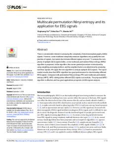
Figure 1: Coarse-grained procedure.

Thus, each pair of weight value 𝑤𝑖 and motif type 𝜋𝑘 can represent full feature for each vector 𝑋𝑖𝑚 . By using weight value, WPE extends the concept of PE with the addition of amplitude information prior to the computing of probability occurrence of each motif defined in (6). Weighted relative frequency is defined as 𝑝𝑤 (𝜋𝑘 ) =

∑ {𝑤𝑖 | 1 ≤ 𝑖 ≤ 𝑁 − (𝑚 − 1) 𝜏, 𝑋𝑖𝑚 has type 𝜋𝑘 } (8) . ∑ 𝑤𝑖

Then WPE of time series 𝑥(𝑛) is 𝐾

𝐻WPE (𝑚) = − ∑ 𝑝𝑤 (𝜋𝑘 ) ln 𝑝𝑤 (𝜋𝑘 ) .

(9)

𝑘=1

2.3. Multiscale Weighted Permutation Entropy. Multiscale analysis [22] is to obtain new time series of the original time series by a coarse-grained size process, which can estimate the complexity of time signals at different scales. Multiscale weighted permutation entropy (MWPE) is the combination of weighted permutation entropy and multiscale analysis. MWPE can totally describe the microstructure complexity and amplitude information of the time series on multiscale. The MWPE procedure is summarized in the following steps. Firstly, the original time series 𝑥(𝑛) = {𝑥1 , 𝑥2 , . . . , 𝑥𝑁} is divided into nonoverlapping windows of length 𝑠. Secondly, the data points inside each window are averaged by (10), and the coarse-grained time series 𝑦𝑗𝑠 is got. The schematic illustration of the coarse-grained procedure is shown in Figure 1. Consider the following: 𝑦𝑗𝑠

𝑗𝑠

1 𝑁 = ∑ 𝑥, 1≤𝑗≤ . 𝑠 𝑖=(𝑗−1)𝑠+1 𝑖 𝑠

(10)

Weighted permutation entropy of 𝑦𝑗𝑠 is MWPE, as shown in MWPE (𝑥, 𝑠, 𝑚, 𝜏) = WPE (𝑦𝑗𝑠 , 𝑚, 𝜏) .

(11)

MWPE is a function of scale factor 𝑠 and represents the complexity of time series on each scale. When 𝑠 = 1, MWPE

is the same as WPE; that is to say, WPE is a special form of MWPE. For most of signals, the MWPE on one single scale is not enough to describe complexity of the signal, and the multiscale weighted permutation entropy is more suitable for the analysis of all kinds of actual signals. 2.4. Parameters Selection. Before computing multiscale weighted permutation entropy, four important parameters including the length 𝑁 of time series data, embedding dimension 𝑚, time delay 𝜏, and scale factor 𝑠 are needed to set. The value of PE mainly depends on the embedding dimension 𝑚 and time delay 𝜏. Embedding dimension 𝑚 determines the number of sequential pattern, and the maximum sequential pattern number is 𝑚!, so 𝑚 plays an important role in calculating the probability of the sequential pattern. If embedding dimension is too small (such as less than 3), it is hard to differentiate the sequential patterns. If the embedding dimension 𝑚 is too large (such as more than 8), calculation of PE is time consuming, and it is not easy to observe the small changes in the signal [16]. The time delay 𝜏 is related to the sampling rate of the signal. As [8] suggests, the time delay 𝜏 is set to 1 in this paper. The length of time series 𝑁 has a great influence on the calculation of PE, a larger 𝑁 will cause low computational efficiency, and a smaller 𝑁 cannot completely describe the complexity of the time series. 𝑁 ≥ 5𝑚! is recommended by [9]. To illustrate the rationality of parameters selection, some experiments are conducted. The experiment data used in this paper is 1-minute gas sensor data. Sampling rate is 100 Hz and the data has 6000 sampling points. Given that the scale factor 𝑠 is a fixed value, Figure 2 shows the weighted permutation entropy (WPE) of four kinds of sensor data under different embedding dimensions, m = 2–8, and the time delay 𝜏 = 1. As shown in Figure 2, when 𝑚 = 5, WPE can separate the four kinds of signals. So 𝑚 = 5 is feasible and is used in this paper. In Figure 3, it is easy to find that different 𝜏 almost has no effect on WPE, so it is reasonable for the fact that 𝜏 is set to 1. In this paper, the scale factor 𝑠 is set to 20. MWPEs on 20 scales are used as the features to identify and classify faults.

4

Journal of Sensors 7

So the combination of wavelet transform with MWPE can comprehensively describe the multiple features of the signal.

6

WPE

5 4 3 2 1 0

2

3

Normal Bias

4 5 6 Embedding dimension m

7

8

Stuck-at Drift

3.1. WMWPE. Given the analyzed signal 𝑥(𝑛) and wavelet decomposed level 𝐽, wavelet decomposed coefficients are expressed as {𝐷1 (𝑛), 𝐷2 (𝑛), . . . , 𝐷𝐽 (𝑛), 𝐴 𝐽 (𝑛)}, corresponding to the coefficients 𝐷1 (𝑛) of the first high frequency subband (HF1 ), the coefficients 𝐷2 (𝑛) of the second high frequency subband (HF2 ), . . ., the coefficients 𝐷𝐽 (𝑛) of the 𝐽 high frequency subband (HF𝐽 ), and the coefficients 𝐴 𝐽 (𝑛) of the 𝐽 low frequency subband (LF𝐽 ). 𝐴 𝐽 (𝑛) belongs to the low frequency subband, which represents the macrostructure of the analyzed signal. So 𝐴 𝐽 (𝑛) is the preferable subband to calculate WMWPE: WMWPE (𝐴 𝐽 (𝑛) , 𝑠, 𝑚, 𝜏) = WPE (𝑦𝑗𝑠 , 𝑚, 𝜏) ,

(12)

𝑗𝑠

where 𝑦𝑗𝑠 = (1/𝑠) ∑𝑖=(𝑗−1)𝑠+1 𝐴 𝐽 (𝑛), 1 ≤ 𝑗 ≤ 𝑁𝐽 /𝑠, 𝑁𝐽 is the number of coefficients in LF𝐽 , and 𝑠 is the scale factor.

Figure 2: The relationship of 𝑚 and WPE.

3.2. WMWPE Based Fault Identification Method. The WMWPE based fault identification method takes advantage of wavelet transform, WMWPE, MCFS, and BP-NN. It provides a full working flow of feature selection and fault identification as shown in Figure 4. Detailed procedures are described as follows.

7 6

WPE

5

Step 1. Use maximum energy-to-Shannon entropy ratio criterion to choose a proper wavelet base.

4

Step 2. The sensor signals are decomposed by the selected wavelet base. A series of wavelet subband signals are obtained, and the appropriate subband signal is selected to extract feature.

3 2

Step 3. Calculate multiscale weighted permutation entropy of the selected wavelet subbands, and WMWPEs are got.

1 0

2

3 𝜏= 𝜏= 𝜏= 𝜏= 𝜏=

1 2 3 4 5

4 5 6 Embedding dimension m 𝜏= 𝜏= 𝜏= 𝜏= 𝜏=

7

8

6 7 8 9 10

Figure 3: The relationship of 𝜏 and WPE.

3. Wavelet Based Multiscale Weighted Permutation Entropy (WMWPE) and Fault Identification Method Although the MWPE takes advantage of the local microstructure information and amplitude information of signal, the macrostructure information is not explored. Wavelet transform is a powerful method to explore it and can be used to extract the global macrostructure information of the signal.

Step 4. After feature extraction, calculate MCFS score of the WMWPE features. According to the MCFS score ranked from high to low, select the features corresponding to the top 𝐾 MCFS score as the best subset of features. Step 5. The selected 𝐾 features by MCFS are fed into BP-NN classifier for sensor fault recognition.

4. Experiments and Result Analysis In this paper, the experimental data set is the measurement recordings collected from an array of 72 metal-oxide gas sensor array-based chemical detection platform [25]. The sampling rate of data is 100 Hz. One-minute sampling data (6000 sampling points) of each sensor is used as original data. Three kinds of fault (bias, stuck-at, and drift) are injected into original data. Each kind has 120 groups of data. For bias fault, the bias constant is 2% of the average value of original data. In each stuck-at fault, there are two segments of data with constant value (98% of the average value of the original). In drift fault groups, drift rate is 0.1% of the average value of

Journal of Sensors

5

The signal to be identified

Using maximum energy-to-Shannon entropy ratio criterion to choose a proper wavelet base

Wavelet transform

A J (n) of the J level low frequency subband

D1 (n) of the first high frequency subband

···

DJ (n) of the J level high frequency subband

Selecting proper subband

Feature extraction

Calculate WMWPEs

Calculate MCFS of WMWPEs and select the features corresponding to the top K MCFS as the best subset of features Feature selection

BP-NN classifier

Output type of fault Fault recognition

Figure 4: Flowchart of sensor fault feature extraction and recognition method.

original data. Normal sensor data and fault sensor data are shown in Figure 5, respectively. (1) Selection of Wavelet Subband. Before selection of wavelet subband, the maximum energy-to-Shannon entropy ratio criterion is used for wavelet base selection. More detailed information can be found in [26]. Figure 6 is the average WMWPE of 120 sensor signals after 3-level wavelet decomposition. It is easy to find that WMWPE of the low frequency subband can easily differentiate the four kinds of sensor signals (normal, bias, stuck-at, and drift) on different scale factor 𝑠, and WMWPE of three high frequency subbands cannot distinguish the four kinds of sensor signals. The experiment results show that selecting the low frequency subband for feature extraction is feasible. (2) Feature Extraction and Fault Identification. After 3-level wavelet decomposition, feature extraction on the third-level

low frequency subband is the further job. The WMWPEs of the selected low frequency subband signal on 20 scales are calculated. These WMWPEs will be fed into BP-NN classifier to identify fault. A three-layer BP-NN neural network is used as classifier in the experiments. The hidden layer of the network has 10 neural nodes for learning. The network is trained by scaled conjugate gradient back-propagation method. Mean squared error is used as performance function. To obtain the generalized identification performance, 10-fold cross-validation [27, 28] is used in this paper. In 10-fold cross-validation, the proposed feature vectors are randomly partitioned into 10 equal sized subsets. Of the 10 subsets, a single subset is retained as the validation data for testing, and the remaining 9 subsets are used as training data. The cross-validation process is then repeated 10 times, with each of the 10 subsets used exactly once as the validation data. The 10 results from the folds can then be averaged to produce a single estimation.

Journal of Sensors 876

895

875

890

Amplitude (ppmv)

Amplitude (ppmv)

6

874 873 872 871 870

0

10

20

30 Time (s)

40

50

885 880 875 870

60

0

10

20

(a)

Amplitude (ppmv)

Amplitude (ppmv)

885 880 875 0

10

20

40

50

60

40

50

60

(b)

890

870

30 Time (s)

30 Time (s)

40

50

60

(c)

880 878 876 874 872 870

0

10

20

30 Time (s) (d)

Figure 5: Normal sensor data and fault sensor data. (a) Normal data, (b) bias, (c) stuck-at, and (d) drift.

Table 1: Average identification accuracy and standard deviation of 20 WMWPEs of different subband. Subband LF3 HF1 HF2 HF3

Average identification accuracy ± standard deviation 99.50% ± 0.08 60.94% ± 1.42 72.99% ± 0.64 76.11% ± 0.65

Table 2: Identification results of WMWPE feature of LF3 subband. Actual type Normal Bias Stuck-at Drift

Identification results Normal Bias Stuck-at Drift 99.43% ± 0.24 0% 0% 0.57% ± 0.24 0% 100% 0% 0% 0% 0% 100% 0% 1.18% ± 0.17 0.28% ± 0.02 0% 98.54% ± 0.16

To illustrate the identification performance of WMWPE on different subbands (HF1 , HF2 , HF3 , and LF3 ), all WMWPEs of 20 scales are used to recognize faults. Table 1 shows the average identification accuracy of different subband. WMWPE of LF3 has much better identification performance than that of other subbands. The average identification accuracy of LF3 is 99.5% and about 20% higher than others. At the same time, LF3 has the smallest identification standard deviation than others. It explains the rationality of selecting WMWPE of LF3 subband as features. Table 2 is the detailed identification results of WMWPE from LF3 subband. For bias and stuck-at, the identification

accuracy is 100%. There is false judgment in the identification of normal and drift signal. The reason is that the local structure pattern and the amplitude of bias and stuck-at are significantly different from those of normal signal. So it is easy to use WMWPE to identify them. Although the drift causes the change of signal amplitude, small change of the amplitude may bring little change to the sequential pattern. And some false negative results exists. (3) Feature Selection. There exists large consuming time and information redundancy, if selecting all 20 scales of WMWPE as features and implementing classification. In order to improve the efficiency of the proposed method, MCFS is used to reduce the dimension of feature vector. After calculating MCFS of 20 WMWPE features, the top 𝐾 features with larger MCFS score are selected as the inputs of BP-NN. The feature selection result and the corresponding identification accuracy are shown in Table 3. Table 3 shows that the average identification accuracy and standard deviation obtained by 5 new selected features are almost the same as those of all 20 features. The experiment results show that, using feature selection algorithm MCFS, the dimension of the feature vector is reduced from 20 to 5, but the recognition accuracy is maintained at about 99.5% with standard deviation of 0.08. That is because MCFS not only considers the classification ability of single feature, but also considers the relationship between the features. (4) Performance Comparison of Different Features. In order to further illustrate the superiority of the proposed method, the identification performance of the proposed method WMWPE is compared with that of MWPE, WWPE, WPE,

Journal of Sensors

7 5

5

4.8 4.6

3

WMWPE

WMWPE

4

2

4.4 4.2

1 0

4 0

5

10 Scale factor s

Normal Bias

15

3.8

20

0

5

Normal Bias

Stuck-at Drift

4.4

4.6

4.2

4.4

4

WMWPE

WMWPE

4.6

4.2 4

3.8 3.6

3.8

3.4

3.6

3.2 5

10 Scale factor s

Normal Bias

20

(b)

4.8

0

15

Stuck-at Drift

(a)

5

3.4

10 Scale factor s

15

20

3

0

5

10 Scale factor s

Normal Bias

Stuck-at Drift (c)

15

20

Stuck-at Drift (d)

Figure 6: The average WMWPE of 120 sensor signals after wavelet decomposition. (a) Low frequency-level 3. (b) High frequency-level 1. (c) High frequency-level 2. (d) High frequency-level 3.

Table 3: Average identification accuracy of the selected feature vectors. Feature dimension 𝐾

The scale index of selected features

1 [1] 2 [19, 20] 3 [18, 13, 17] 4 [18, 17, 3, 4] 5 [18, 4, 6, 5, 7] 6 [18, 4, 5, 2, 1, 6] 7 [4, 18, 5, 2, 1, 6, 17] 8 [4, 18, 5, 2, 1, 6, 3, 7] 9 [4, 5, 18, 2, 1, 6, 3, 7, 8] 10 [4, 5, 18, 2, 1, 3, 6, 7, 8, 12] All 20 features [1, . . . , 20]

Average identification accuracy ± standard deviation 83.46% ± 0.53 87.19% ± 0.72 97.42% ± 0.27 98.74% ± 0.23 99.46% ± 0.09 99.37% ± 0.15 99.30% ± 0.08 99.42% ± 0.13 99.33% ± 0.07 99.43% ± 0.10 99.50% ± 0.08

Table 4: Average identification accuracy of using different features. Features WMWPE MWPE WWPE WPE MPE PE

Average identification accuracy ± standard deviation 99.50% ± 0.08 98.06% ± 0.20 83.34% ± 0.62 45.15% ± 0.49 73.42% ± 0.40 35.27% ± 0.20

MPE, and PE, wherein WWPE is WPE of the low frequency subband signal under wavelet decomposition. Table 4 shows the average recognition accuracy and standard deviation for the four kinds of signals using different features over 10 times of 10-fold cross-validation. The more detailed recognition results are shown in Table 5.

8

Journal of Sensors Table 5: Identification results of different features.

Actual type

Normal

Normal Bias Stuck-at Drift

97.93% ± 0.56 0% 0% 1.43% ± 0.2


90.87% ± 0.52 0% 0% 26.83% ± 0.96


40.87% ± 6.97 15.70% ± 2.05 6.2% ± 1.31 42.80% ± 6.35


57.76% ± 1.40 42.06% ± 0.82 3.20% ± 0.44 4.50% ± 0.08

Identification results Bias Stuck-at MWPE 0% 0% 98.13% ± 0.48 1.87% ± 0.46 1.43% ± 0.23 98.57% ± 0.22 0.8% ± 0.3 0% WWPE 0% 0% 74.5% ± 1.62 25.50% ± 1.51 3.67% ± 0.21 96.33% ± 0.26 0% 1.47% ± 0.41 WPE 13.03% ± 1.43 6.97% ± 0.82 35.30% ± 4.52 27% ± 3.63 20.47% ± 2.95 64.13% ± 2.71 10.70% ± 1.60 6.20% ± 0.84 MPE 37.91% ± 1.38 4.33% ± 0.17 53.74% ± 0.71 4.20% ± 0.32 10.13% ± 1.42 86.67% ± 1.42 0% 0%

Drift 2.07% ± 0.51 0% 0% 97.77% ± 0.19 9.13% ± 0.46 0% 0% 71.7% ± 1.34 39.13% ± 7.42 22% ± 2.85 9.20% ± 1.47 40.30% ± 6.76 0% 0% 0% 95.50% ± 0.24

As shown in Tables 2, 4, and 5, the identification accuracy of WMWPE is higher than that of MWPE. The same conclusion can be got from the performance comparison of WWPE with WPE. That is because wavelet transform brings macrostructure information into the feature. Combined with macro- and microstructure information, WMWPE and WWPE can get better performance. Comparing the results of WMWPE to WWPE, MWPE to WPE, and MPE to PE, the multiscales analysis can improve the identification precision over 16%. The main reason is that the multiscale feature can explore more local structure information of the signals than the single scale feature. Comparing the results of MWPE to MPE and WPE to PE, the amplitude information can bring about 25% and 9% increase of average identification accuracy, respectively. So the macro- and microstructure information and amplitude information are all explored by WMWPE. The experiment results validate that the proposed method based on WMWPE can achieve high identification accuracy for sensor fault.

extraction, multicluster feature selection, and BP classifier are investigated. Actual chemical gas concentration data is used to evaluate the performance of the proposed method. Experiment results show that the proposed WMWPE extracts more comprehensive feature information and can achieve higher fault recognition accuracy than other kinds of features.

5. Conclusion

[3] M. Zhang, J. Wu, and Y. Wang, “Sensor soft fault detection method of autonomous underwater vehicle,” in Proceedings of the IEEE International Conference on Mechatronics and Automation (ICMA ’09), pp. 4839–4844, Changchun, China, August 2009.

How to find an effective feature extraction method for sensor fault analysis and identification is always an important issue. Taking full advantage of macrostructure information, microstructure information, and amplitude information of the typical sensor faults, this paper proposed a new sensor fault feature extraction and identification method based on wavelet transform and multiscale weighted permutation entropy. The appropriate based wavelet selection, feature

Competing Interests The authors declare no competing interests.

References [1] G. Heredia and A. Ollero, “Sensor fault detection in small autonomous helicopters using observer/Kalman filter identification,” in Proceedings of the IEEE International Conference on Mechatronics (ICM ’09), pp. 1–6, April 2009. [2] J. C. D. Silva, A. Saxena, E. Balaban, and K. Goebel, “A knowledge-based system approach for sensor fault modeling, detection and mitigation,” Expert Systems with Applications, vol. 39, no. 12, pp. 10977–10989, 2012.

[4] H. Liu, M. Huang, I. Janghorban, P. Ghorbannezhad, and C. Yoo, “Faulty sensor detection, identification and reconstruction of indoor air quality measurements in a subway station,” in Proceedings of the 11th International Conference on Control, Automation and Systems (ICCAS ’11), pp. 323–328, October 2011.

Journal of Sensors [5] W. He, Q. Miao, M. Azarian, and M. Pecht, “Health monitoring of cooling fan bearings based on wavelet filter,” Mechanical Systems and Signal Processing, vol. 64-65, pp. 149–161, 2015. [6] R. Yan, Base wavelet selection criteria for non-stationary vibration analysis in bearing health diagnosis [Ph.D. thesis], University of Massachusetts Amherst, Amherst, Mass, USA, 2007. [7] P. K. Kankar, S. C. Sharma, and S. P. Harsha, “Fault diagnosis of ball bearings using continuous wavelet transform,” Applied Soft Computing Journal, vol. 11, no. 2, pp. 2300–2312, 2011. [8] C. Bandt and B. Pompe, “Permutation entropy: a natural complexity measure for time series,” Physical Review Letters, vol. 88, no. 17, Article ID 174102, 2002. [9] M. Zanin, L. Zunino, O. A. Rosso, and D. Papo, “Permutation entropy and its main biomedical and econophysics applications: a review,” Entropy, vol. 14, no. 8, pp. 1553–1577, 2012. [10] W. Aziz and M. Arif, “Multiscale permutation entropy of physiological time series,” in Proceedings of the Pakistan Section Multitopic Conference, pp. 1–6, Karachi, Pakistan, December 2005. [11] S.-D. Wu, P.-H. Wu, C.-W. Wu, J.-J. Ding, and C.-C. Wang, “Bearing fault diagnosis based on multiscale permutation entropy and support vector machine,” Entropy, vol. 14, no. 8, pp. 1343–1356, 2012. [12] P. L. Vuong, A. S. Malik, and J. Bornot, “Weighted-permutation entropy as complexity measure for electroencephalographic time series of different physiological states,” in Proceedings of the 3rd IEEE Conference on Biomedical Engineering and Sciences (IECBES ’14), pp. 979–984, Kuala Lumpur, Malaysia, December 2014. [13] B. Fadlallah, B. Chen, A. Keil, and J. Principe, “Weightedpermutation entropy: a complexity measure for time series incorporating amplitude information,” Anesthesiology, vol. 87, no. 2, pp. 1647–1650, 2013. [14] X. Chen, N.-D. Jin, A. Zhao, Z.-K. Gao, L.-S. Zhai, and B. Sun, “The experimental signals analysis for bubbly oil-in-water flow using multi-scale weighted-permutation entropy,” Physica A: Statistical Mechanics & its Applications, vol. 417, pp. 230–244, 2015. [15] J. Zhou, J. Xiao, H. Xiao, W. Zhang, W. Zhu, and C. Li, “Multifault diagnosis for rolling element bearings based on intrinsic mode permutation entropy and ensemble optimal extreme learning machine,” Advances in Mechanical Engineering, vol. 6, Article ID 803919, 2014. [16] R. Yan, Y. Liu, and R. X. Gao, “Permutation entropy: a nonlinear statistical measure for status characterization of rotary machines,” Mechanical Systems and Signal Processing, vol. 29, pp. 474–484, 2012. [17] X. Zhang, Y. Liang, J. Zhou, and Y. Zang, “A novel bearing fault diagnosis model integrated permutation entropy, ensemble empirical mode decomposition and optimized SVM,” Measurement, vol. 69, pp. 164–179, 2015. [18] C. Bian, C. Qin, Q. D. Y. Ma, and Q. Shen, “Modified permutation-entropy analysis of heartbeat dynamics,” Physical Review E—Statistical, Nonlinear, and Soft Matter Physics, vol. 85, no. 2, Article ID 021906, pp. 439–441, 2012. [19] U. Parlitz, S. Berg, S. Luther, A. Schirdewan, J. Kurths, and N. Wessel, “Classifying cardiac biosignals using ordinal pattern statistics and symbolic dynamics,” Computers in Biology and Medicine, vol. 42, no. 3, pp. 319–327, 2012. [20] N. Nicolaou and J. Georgiou, “Detection of epileptic electroencephalogram based on permutation entropy and support vector

9

[21]

[22]

[23]

[24]

[25]

[26]

[27]

[28]

Machines,” Expert Systems with Applications, vol. 39, no. 1, pp. 202–209, 2012. A. Ravelo-Garc´ıa, J. Navarro-Mesa, U. Casanova-Blancas et al., “Application of the permutation entropy over the heart rate variability for the improvement of electrocardiogram-based sleep breathing pause detection,” Entropy, vol. 17, no. 3, pp. 914– 927, 2015. Y. Yin and P. Shang, “Weighted multiscale permutation entropy of financial time series,” Nonlinear Dynamics, vol. 78, no. 4, pp. 2921–2939, 2014. D. Cai, C. Zhang, and X. He, “Unsupervised feature selection for multi-cluster data,” in Proceedings of the 16th ACM SIGKDD International Conference on Knowledge Discovery and Data Mining (KDD ’10), pp. 333–342, ACM, Washington, DC, USA, July 2010. M. Kang, M. R. Islam, J. Kim, J.-M. Kim, and M. Pecht, “A hybrid feature selection scheme for reducing diagnostic performance deterioration caused by outliers in data-driven diagnostics,” IEEE Transactions on Industrial Electronics, vol. 63, no. 5, pp. 3299–3310, 2016. “Gas sensor arrays in open sampling settings Data set,” 2016, https://archive.ics.uci.edu/ml/datasets/Gas+sensor+arrays+in +open+sampling+settings. Q. Yang and J. Wang, “Multi-level wavelet shannon entropybased method for single-sensor fault location,” Entropy, vol. 17, no. 10, pp. 7101–7117, 2015. J. Rodriguez, A. Perez, and J. Lozano, “Sensitivity analysis of k-fold cross validation in prediction error estimation,” IEEE Transactions on Pattern Analysis and Machine Intelligence, vol. 32, no. 3, pp. 569–575, 2010. M. Kang, J. Kim, J.-M. Kim, A. C. C. Tan, E. Y. Kim, and B.-K. Choi, “Reliable fault diagnosis for low-speed bearings using individually trained support vector machines with kernel discriminative feature analysis,” IEEE Transactions on Power Electronics, vol. 30, no. 5, pp. 2786–2797, 2015.

International Journal of

Rotating Machinery

Engineering Journal of

Hindawi Publishing Corporation http://www.hindawi.com

Volume 2014

The Scientific World Journal Hindawi Publishing Corporation http://www.hindawi.com

Volume 2014


Distributed Sensor Networks

Journal of

Sensors Hindawi Publishing Corporation http://www.hindawi.com

Volume 2014


Volume 2014


Volume 2014

Journal of

Control Science and Engineering

Advances in

Civil Engineering Hindawi Publishing Corporation http://www.hindawi.com


Volume 2014

Volume 2014

Submit your manuscripts at http://www.hindawi.com Journal of

Journal of

Electrical and Computer Engineering

Robotics Hindawi Publishing Corporation http://www.hindawi.com


Volume 2014

Volume 2014

VLSI Design Advances in OptoElectronics


Navigation and Observation Hindawi Publishing Corporation http://www.hindawi.com

Volume 2014



Chemical Engineering Hindawi Publishing Corporation http://www.hindawi.com

Volume 2014

Volume 2014

Active and Passive Electronic Components

Antennas and Propagation Hindawi Publishing Corporation http://www.hindawi.com

Aerospace Engineering


Volume 2014


Volume 2014

Volume 2014




Modelling & Simulation in Engineering

Volume 2014


Volume 2014

Shock and Vibration Hindawi Publishing Corporation http://www.hindawi.com

Volume 2014

Advances in

Acoustics and Vibration Hindawi Publishing Corporation http://www.hindawi.com

Volume 2014