A Web-Based Environment for Learning

A Web-Based Environment for Learning Normalization of Relational Database Schemata Nikolay Georgiev

September 2008 Master’s Thesis in Computing Science, 30 ECTS credits Supervisor at CS-UmU: Stephen J. Hegner Examiner: Per Lindstr¨om

Ume˚ a University Department of Computing Science SE-901 87 UME˚ A SWEDEN

Abstract Database normalization is a technique for designing relational database tables to minimize duplication of information in order to safeguard the database against certain types of logical or structural problems, namely data anomalies. Therefore database normalization is a central topic in database theory, and its correct understanding is crucial for students. Unfortunately, the subject it is often considered to be dry and purely theoretical and is often not well received by students. A web-based environment for learning normalization of relational database schemata is developed to give students an interactive hands-on experience in database normalization process. It also provides lecturers with an easy way for creating and testing assignments on the subject. The environment is suitable for relational database and design and data management courses. This report describes the design and development of LDBN (Learn DataBase Normalization) - a reference implementation of the learning environment. It also discuss problems that lie within educational and web-based software development.

ii

Contents 1 Introduction

1

1.1

Organization of This Report . . . . . . . . . . . . . . . . . . . . . . . . .

2

1.2

Learning Database Normalization with LDBN . . . . . . . . . . . . . . .

2

1.3

Comparation of LDBN with Other Tools . . . . . . . . . . . . . . . . . .

5

1.4

Glossary . . . . . . . . . . . . . . . . . . . . . . . . . . . . . . . . . . . .

5

2 Preliminaries 2.1

2.2

7

Definitions . . . . . . . . . . . . . . . . . . . . . . . . . . . . . . . . . . .

7

2.1.1

Relation . . . . . . . . . . . . . . . . . . . . . . . . . . . . . . . .

7

2.1.2

Key . . . . . . . . . . . . . . . . . . . . . . . . . . . . . . . . . .

8

2.1.3

Functional Dependency . . . . . . . . . . . . . . . . . . . . . . .

9

2.1.4

Closure of a Set of FDs . . . . . . . . . . . . . . . . . . . . . . .

9

2.1.5

Formal Definition of Keys . . . . . . . . . . . . . . . . . . . . . .

10

2.1.6

Cover of Sets of FDs . . . . . . . . . . . . . . . . . . . . . . . . .

10

2.1.7

Decomposition of Relations . . . . . . . . . . . . . . . . . . . . .

11

Brief Introduction to the Normal Forms . . . . . . . . . . . . . . . . . .

13

2.2.1

Data Anomalies

. . . . . . . . . . . . . . . . . . . . . . . . . . .

13

2.2.2

First Normal Form . . . . . . . . . . . . . . . . . . . . . . . . . .

13

2.2.3

Second Normal From . . . . . . . . . . . . . . . . . . . . . . . . .

15

2.2.4

Third Normal Form . . . . . . . . . . . . . . . . . . . . . . . . .

16

2.2.5

Boyce-Codd Normal Form . . . . . . . . . . . . . . . . . . . . . .

17

3 Design Concepts

19

3.1

Choice of Platform . . . . . . . . . . . . . . . . . . . . . . . . . . . . . .

19

3.2

AJAX . . . . . . . . . . . . . . . . . . . . . . . . . . . . . . . . . . . . .

20

3.3

GWT . . . . . . . . . . . . . . . . . . . . . . . . . . . . . . . . . . . . .

21

3.4

Limitations of GWT and JavaScript . . . . . . . . . . . . . . . . . . . .

24

3.5

Server-side Platform Choice . . . . . . . . . . . . . . . . . . . . . . . . .

24

3.6

Other Design Issues . . . . . . . . . . . . . . . . . . . . . . . . . . . . .

24

iii

iv

4 Implementation 4.1 System Architecture . . . . . . . . 4.2 Core Package of LDBN . . . . . . . 4.3 Normalization Algorithms . . . . . 4.3.1 Algorithms for Testing . . . 4.3.2 Decomposition Algorithms 4.4 Key Functions of LDBN . . . . . . 4.5 User Interface . . . . . . . . . . . . 4.6 Server Side . . . . . . . . . . . . . 4.7 Security Issues . . . . . . . . . . .

CONTENTS

. . . . . . . . .

25 25 27 29 31 38 40 43 46 47

5 Conclusions 5.1 Limitations and Future Work . . . . . . . . . . . . . . . . . . . . . . . .

49 50

6 Acknowledgements

51

References

53

. . . . . . . . .

. . . . . . . . .

. . . . . . . . .

. . . . . . . . .

. . . . . . . . .

. . . . . . . . .

. . . . . . . . .

. . . . . . . . .

. . . . . . . . .

. . . . . . . . .

. . . . . . . . .

. . . . . . . . .

. . . . . . . . .

. . . . . . . . .

. . . . . . . . .

. . . . . . . . .

. . . . . . . . .

. . . . . . . . .

. . . . . . . . .

. . . . . . . . .

List of Figures 1.1 1.2 1.3

Solve Assignments Tab . . . . . . . . . . . . . . . . . . . . . . . . . . . . Load Assignments List . . . . . . . . . . . . . . . . . . . . . . . . . . . . Check Solution Dialog . . . . . . . . . . . . . . . . . . . . . . . . . . . .

2.1 2.2 2.3 2.4 2.5 2.6

Relation Example . . . . . . . . . . . . . . . . . . . . . . . Lossless-Join Property Example . . . . . . . . . . . . . . . Relation Student Courses . . . . . . . . . . . . . . . . . . Set of FDs which hold in Student Courses . . . . . . . . . Decomposition of Relation Student Courses in 2NF . . . . Decomposition of Relation Students and Mentors in 3NF

. . . . . .

8 12 14 15 16 17

3.1 3.2 3.3

Example of an AJAX Architecture . . . . . . . . . . . . . . . . . . . . . AJAX Architectural Shift . . . . . . . . . . . . . . . . . . . . . . . . . . GWT Java-to-JavaScript Compiler . . . . . . . . . . . . . . . . . . . . .

21 21 22

4.1 4.2 4.3 4.4 4.5 4.6 4.7 4.8 4.9 4.10 4.11 4.12 4.13 4.14 4.15 4.16

System Architecture of LDBN . . . . . . . . . . . . . . . Example of a Relation Representation in LDBN . . . . . UML Class Diagram of LDBN’s Core Classes . . . . . . Pseudocode for Algorithm Classical-AttributeClosure . . Pseudocode for Algorithm SLFD-Closure . . . . . . . . Pseudocode for Algorithm FDTest . . . . . . . . . . . . Pseudocode for Algorithm Equivalence . . . . . . . . . . Pseudocode for Algorithm TestLosslessJoin . . . . . . . Pseudocode for Algorithm TestDependencyPreservation Pseudocode for Algorithm FindAllCandidateKeys . . . . Pseudocode for Algorithm ReductionByResolution . . . Pseudocode for Algorithm FindMinimalCover . . . . . . Pseudocode for Algorithm Decomposition3NF . . . . . . Pseudocode for Algorithm DecompositionBCNF . . . . Order of the Decomposition Algorithms . . . . . . . . . Home View . . . . . . . . . . . . . . . . . . . . . . . . .

26 28 30 31 32 32 33 34 35 36 37 39 40 41 42 44

v

. . . . . . . . . . . . . . . .

. . . . . .

. . . . . . . . . . . . . . . .

. . . . . .

. . . . . . . . . . . . . . . .

. . . . . .

. . . . . . . . . . . . . . . .

. . . . . .

. . . . . . . . . . . . . . . .

. . . . . .

. . . . . . . . . . . . . . . .

. . . . . .

. . . . . . . . . . . . . . . .

. . . . . .

. . . . . . . . . . . . . . . .

. . . . . . . . . . . . . . . .

3 4 4

vi

LIST OF FIGURES

4.17 4.18 4.19 4.20 4.21

Solve Assignments View . . . . Create Assignments View . . . Attribute and Key Editor . . . FD Editor and an Example of a Help Dialog for the FD Editor

. . . . . . . . . . . . . . . . . . . . . . . . . . . . . . . . . Relation in LDBN . . . . . . . . . . .

. . . . .

. . . . .

. . . . .

. . . . .

. . . . .

. . . . .

. . . . .

. . . . .

. . . . .

. . . . .

. . . . .

. . . . .

44 45 45 46 47

Chapter 1

Introduction Readers unfamiliar with the terms of relational-database normalization and functional dependencies can find a brief introduction on the subject in Chapter 2. Due to its great importance for database applications database schema design has attracted substantial research [18]. Relational-database normalization is a theoretical approach for structuring a database schema and it is very well developed. Unfortunately, theory is not yet understood well by practitioners [18]. One of the reasons for this is the lack of good tools which could aid the students during the learning process of relationaldatabase normalization [31]. Thus our learning environment was developed in order to give students the ability to easily and efficiently test their knowledge of the different normal forms in practice. The environment assists the students by providing them the following functionalities: 1. Allow the student to specify a candidate decomposition of a given relation. 2. Assess the correctness of the student’s proposed decomposition relative to many factors; including: – Lossless-join property. – Dependency preservation. – Specification of keys. – Correctness of the Second Normal Form (2NF), Third Normal Form (3NF) and Boyce-Codd Normal Form (BCNF) decompositions. 3. Provide students with sample decompositions when needed. 4. Allow users to communicate with each other via comments/posts. Our learning environment uses many different normalization algorithms for achieving the functionalities described above. We can divide them into two different groups: Decomposition algorithms are used for decomposing a normalized database schema into a certain normal form using functional dependencies (FDs). Test algorithms for testing whether a given relational schema violates certain normal form, the lossless-join property or other criteria. 1

2

Chapter 1. Introduction

A given schema may have many decompositions into a given normal form. Therefore, simply computing one such decomposition and comparing the student’s solution to it is not satisfactory. Rather, what is needed are test algorithms which check a decomposition proposed by the student for correctness. Here it is worth mentioning that the normalization algorithms often require background in relational algebra that most IS/IT students lack [31]. This is also an issue which our tool addresses by providing a more intuitive way of decomposing a schema and by giving an easy way for lecturers to teach by example and test the knowledge of their students.

1.1

Organization of This Report

In the remaining sections of this chapter we introduce informally the key features and concepts of our web-based learning environment, called LDBN (Learn DataBase Normalization) [6]; compare it to a couple of other available web-based database normalization tools, and provide the reader with small glossary. In Chapter 2 we give definitions to relational-database normalization and to the different normal forms. In Chapter 3 we discuss some design issues regarding LDBN such as platform choice and others. Chapter 4 provides a formal description of our reference implementation of the learning environment, and Chapter 5 shows our conclusions.

1.2

Learning Database Normalization with LDBN

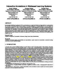
In this section we briefly introduce our reference implementation of the web-based learning environment, called LDBN. Figure 1.1 shows the overview of the most important part of the user interface (UI) - the Solve Assignment view/tab. Here students can test their knowledge on the subject of relational-database normalization. The first thing the reader may notice is the fact that LDBN runs within a browser. The client side of LDBN is written in JavaScript following the AJAX techniques (more about this in Chapter 3). Furthermore, LDBN is assignment driven. This means students have to first choose an assignment from a list with assignments, submitted by other users (lecturers). Such a list is shown in Figure 1.2. An assignment consists of a relational-database schema in universal-relation form (URF), i.e., all the attributes in a single relation and a set of FDs on the attributes. After an assignment has been loaded, we require the students to go through the following steps in LDBN: 1. Determine a minimal cover of the given FDs, also known as a canonical cover. 2. Decompose the relational schema which is in URF into 2NF, 3NF and BCNF. 3. Determine a primary key for each new relation/table. The task of checking a potential solution involves many subtasks, which may be performed in any order. In addition to this, a partial or complete solution can be submitted at any given time by pressing the Check Solution button. After that the system analyzes the solution by performing the following checks: 1. Correctness of the minimal cover of the given FDs.

1.2. Learning Database Normalization with LDBN

3

Figure 1.1: Solve Assignments Tab

2. Correctness of the FDs associated with each relation R; that is, if the FDs are actually in the embedded closure of FR+ for this relation. See Section 2.1.4 for more details on a closure of a set of FDs. 3. Losses-join properly for every schema in the decomposition. 4. Dependency preservation for every decomposition. 5. Correctness of the key of each relation. 6. Correctness of the decomposition, i.e., if the decomposition is really in 2NF, 3NF and BCNF. A dialog with the result is shown to the user. In case of an error the system offers feedback in form of small textual hints, indicating where the error might be. Such a

4


Figure 1.2: Load Assignments List

Figure 1.3: Check Solution Dialog

dialog is shown in Figure 1.3. In this case we can see that the user has made a correct decomposition for 2NF and 3NF, but his/her decomposition for BCNF has some errors, namely the key of the relation R4 is incorrect. The dialog shows that the decomposition does not satisfy the dependency-preservation property, but in the case of BCNF this is not always possible, therefore it is only a warning. Additional features of LDBN include creating an assignment, which can be done only by registered users. This restriction is necessary in order users to be able to distinct assignments provided by trusted users, e.g. the database course lecturers. Registered users have also the ability to leave textual comments for every assignment. On the one hand, such comments ensure that user can easily communicate and share ideas with each other, and one the other hand, comments could also decrease the amount of workload for the lecturers in terms of giving an explanation to difficult decomposition. More detailed and formal description of the features of LDBN will be given in Chapter 4.

1.3. Comparation of LDBN with Other Tools

1.3

5

Comparation of LDBN with Other Tools

In this section we compare LDBN to a couple of other available web-based database normalization tools such as the Web-based Tool to Enhance Teaching/Learning Database Normalization by Kung [31] and the The Database Normalization Tool [9]. Furthermore, we discuss why we think our tool is better and more efficient in terms of teaching potential, and give possible reasons why the other tools are not commonly used by students. First of all, the concept of assignments is a major difference between LDBN and the other normalization tools, which only provide one possible solution (decomposition) to the user, without users having the ability to test themselves. On the other hand, LDBN can be used for checking the correctness of any proposed decomposition. This could be useful for lectures to test handwritten assignments. Another major advantage of LDBN over the other tools is the user interface (UI). As Frye [24] and Dantin [21] stated, this is often a neglected feature when it comes to educational software. The lack of user-friendly UI can often lead to unpopularity of the software among students. An example here could be The Database Normalization Tool [9]. Inputting a relational schema in the program can take quite some time due to the fact that users have to input every attribute manually using the keyboard and then also have to input every FD the same way. This may take several minutes even for small assignments. Furthermore, relational schemas cannot be saved for future use as in LDBN, and users have to input them again next time. To overcome this slow input of user data, LDBN supports drag and drop. A feature widely used in desktop applications, but relatively new to an AJAX application such as LDBN. Every attribute and every FD in LDBN can be dragged and dropped, in order to define or modify FDs, key attributes, etc. This ensures a really fast and easy usage of the tool without the need for keyboard input. It should be mentioned that inputting attributes the traditional way by typing them is also supported. Community features such as posting comments are not present in the other two web-based normalization tools, but we believe they are very important when it comes to educational software.

1.4

Glossary

2NF, 3NF, BCNF Second Normal Form, Third Normal Form, Boyce-Codd Normal Form. See Section 2.2 for more details. AJAX Asynchronous JavaScript And XML Asynchronous JavaScript And XML is a group of interrelated web development techniques used for creating interactive web applications, for more details see Section 3.2. API An Application Programming Interface is a set of functions, procedures or classes that an operating system, library or service provides to support requests made by computer programs [10]. CSS Cascading Style Sheets is a stylesheet language used to describe the presentation of a document written in HTML. DBMS A Database Management System is a complex set of software programs that controls the organization, storage, management, and retrieval of data in a database.

6


GWT Google Web Toolkit is an open source Java software development framework that allows web developers to create AJAX applications in Java. More details in Section 3.3. LDBN Learn Database Normalization is our reference implementation of the web-based environment for learning normalization of relational database schemata. We often refer to LDBN as our learning environment or our implementation. ODBC Open Database Connectivity provides a standard software API method for using database management systems. RPC Remote Procedure Call is an inter-process communication technology that allows a computer program to cause a subroutine or procedure to execute in another address space. SQL Structured Query Language is a computer language designed for the retrieval and management of data in relational database management systems, database schema creation and modification, and database object access control management. XMLHttpRequest is an API that can be used by JavaScript and other web browser scripting languages to transfer asynchronously XML and other text data between a web server and a browser.

Chapter 2

Preliminaries In this chapter we give a brief introduction to relational-database normalization. The chapter is intended to be used only as quick reference, since discussing the relational data model and the relational-database normalization in detail is beyond the scope of this report. For readers who would like to read more on the subject we recommend the textbook by Elmasri and Navathe [23] or the textbook by Kemper and Eickler [35] for German-speaking readers, both of which have proven to be helpful guides throughout the development process of LDBN. There are also many free on-line resources such as the article A Simple Guide to Five Normal Forms in Relational Database Theory by Kent [30].

2.1

Definitions

In the following we give some very important definitions to some key concepts in the relational-database normalization, such as relation, key, functional dependency, losslessjoin, 2NF, 3NF, BCNF and others. We also provide the reader with examples to illustrate the different normalization concepts in practice. We follow the notations of Kemper and Eickler [35]. All of the following definitions excluding the examples are also taken from [35, Chapter 6].

2.1.1

Relation

In relational databases data are represented in tables/relations. The columns in the table/relation identify the attributes, for instance in a table for storing personal data of students such attributes could be name, date of birth and so forth. A row or a tuple contains all the data of a single instance of the table such as a student named John Doe. In the relational model, every row must have a unique identification or key based on the data. Figure 2.1 shows an example of a relation in which the Attribute Matriculation Number is the key that uniquely identifies each row/tuple in the relation. We would like to give some more formal definitions as well: Relation Schema: A relation schema is given by a name R, together with a finite set Attr(R) of attributes. For convenience, when no confusion can result, R will be used as an abbreviation for Attr(R). 7

8

Chapter 2. Preliminaries

Figure 2.1: Relation Example

Domain: With each attribute A ∈ Attr(R) is associated a domain Dom(A), that is the set of allowed values for each attribute. Tuple: A tuple over R is a function t on Attr(R) such that t(A) ∈ Dom(A) for each A ∈ Attr(A). For B ⊆ Attr(A), the projection of the tuple t onto B is is the function t restricted to B. This projection often denoted t.B. For B a singleton; i.e., B = {C}, t.C denotes t.{C}. Relation Instance: A relation instance r for a relation schema is a set of tuples over its attribute set. Projection: Projection is a unary operation written as ΠB (r) where B ⊆ Attr(A) and r is an instance of R. ΠB (r) = {t.B|t ∈ r}. In words, it deletes attributes that are not in B. Note that duplicate tuples are automatically eliminated by definition. Natural Join: Natural join is a binary operator that is written as (r o n s) where r and s are relation instances. The result of the natural join is the set of all combinations of tuples in r and s that are equal on their common attribute names. Subsets of Attr(A) are often written using concatenation, when no confusion can result. Thus, if Attr(A) = {A, B, C, D}, then {A, B, C} may also be written ABC. In the following we often use lower-case Greek letters such as α, β and γ to refer to subset of Attr(A).

2.1.2

Key

As we mentioned a key is used to uniquely identify a tuple. Each table can contain more than one key. For example, in our Student relation we could also have an attribute Personal Number which could also be used as a key. Furthermore, each key may be composed from more than one attribute, for instance, all the attributes of every relation always build a key. However, such a key can often be reduced to a smaller subset of the relation’s attributes. We refer to keys that cannot be reduces any more without losing their key property as candidate keys. In addition, each relation has a primary key, which is a selected candidate key for that relation.

2.1. Definitions

2.1.3

9

Functional Dependency

The concept of Functional Dependency (FD) is central to normalization theory. FD is a semantic concept which describes a particular semantic relationship between the attributes of a relation. An FD is often represented as α → β, where α and β are subsets of the attributes of a given relation R. We often refer to α as the left-hand side (LHS) of the FD and to β as the right-hand side (RHS) of the FD. The representation α → β means that for β is functionally dependent on α; that is, for each for each value of α no more than one value of β is associated. More formally, if t and r are two tuples in the relation R with t.α = r.α then t.β = r.β. Here t.α = r.α is a short form for ∀A ∈ α : t.A = r.A. In other words, the values of the attributes in α uniquely determines the values of of the attributes in β and if there were several tuples that had the same value of α then all these tuples will have identical values for the attributes in β. We would like to illustrate this very important concept of FDs with an example. Let us consider the following relation R = {A, B, C, D}. The example comes from [35, Section 6.1]. R t p q r s

A a4 a1 a1 a2 a3

B b2 b1 b1 b2 b2

C c4 c1 c1 c3 c4

D d3 d1 d2 d2 d3

In this instance A → B is satisfied. As all tuples that have the same A value have the same B value. However, B → A is not satisfied, since the tuples r and s with r.B = s.B have different A values. Other FDs on the relation which are also satisfied are A → C and CD → B. A functional dependency is trivial if it satisfied by all tuples, i.e., α → α. In general, a functional dependency of the form α → β is trivial if β ⊆ α.

2.1.4

Closure of a Set of FDs

In a relation schema R constrained by a set F of FDs we define the closure of F , denoted F + , as a set of all possible FDs which can be derived from the original set of FDs F . In other words, F + is the set of all FDs that must always hold in R. F + can be computed using inference rules called Armstrong’s Axioms. Repeated application of these rules will generate all functional dependencies in the closure F + . Let α, β, γ and δ be subsets of the Attributes in R, then: Reflexivity Rule If β ⊆ α then α → β. Augmentation Rule If α → β then αγ → βγ, where αγ is a short form of α ∪ γ. Transitivity Rule If α → β and β → γ then α → γ. Additional rules which can be derived from above axioms: Union Rule If α → β and α → γ then α → βγ.

10


Decomposition Rule If α → βγ then α → β and α → γ. Pseudo Transitivity Rule If α → β and γβ → δ then αγ → δ. Here follows a short example on how to apply the different rules. Let us consider the following relation: R = {A, B, C, G, H, I} F = {A → B, A → C, B → H, CG → H, CG → I} Among others the following FDs can be inferred: A → H by applying the Transitivity Rule: A → B, B → H CG → HI by applying the Union Rule: CG → H, CG → I AG → I by first applying the Augmentation Rule: A → C, AG → CG; and then applying the Transitivity Rule: AG → CG, CG → I

2.1.5

Formal Definition of Keys

With the help of FDs we can now define keys of a relation more formally. But first we define the concept of full functional dependence. Let α and β be sets of attributes. β is fully functionally dependent on α if both of the following criteria are true: 1. α → β holds 2. α cannot be reduced, i.e., ∀A ∈ α : α − {A} 9 β Let R be a relation with α ⊆ R, then α is a superkey if α → R. α is called candidate key if R is fully functional dependent on α. There can be many candidate keys in a relation. Each relation has one primary key, which is a selected candidate key. Furthermore, we define an attribute as prime or key attribute if it is part of some candidate key of R.

2.1.6

Cover of Sets of FDs

Equivalent sets of functional dependencies are called covers of each other. There are many different equivalent sets of FDs. Two sets of FDs F and G are equivalent (F ≡ G) if and only if their closures are equal, i.e., F + = G+ . This means for a given set of FDs F there is only one unique closure F + [35, Section 6.3.1]. Furthermore every set of functional dependencies has a minimal cover Fc . Unlike the closure F + the minimal cover Fc is not unique. A subset Fc ⊆ F is a minimal cover if the following three properties are satisfied: 1. Fc ≡ F , i.e., Fc+ = F + 2. We cannot delete any attribute from any FD and have an equivalent set of FDs. 3. Every left-hand side of each FD must be unique, thus rules with identical LHSs may be combined by combining their RHS. This can be done by successively applying the Union Rule. An example: for the relational scheme R = {A, B, C}, and the set F of functional dependencies:

2.1. Definitions

11

F = {A → BC, B → C, A → B, AB → C} The set Fc = {A → B, B → C} is a minimal cover of F . Proof: 1. F ≡ Fc , by applying the Armstrong’s Axioms it can be shown that A → BC and AB → C are in Fc+ , thus the two sets are equivalent. 2. We cannot remove any attributes from the two FDs in Fc , because by doing so they will become trivial and the resulted set will not be equivalent to Fc . 3. The FDs in Fc differ in their LHSs.

2.1.7

Decomposition of Relations

Relational-database normalization typically involves decomposing a relation R into two Sn or more relations R1 , ..., Rn , with Ri ⊆ R for each i and ( i=1 Ri ) = R, i.e., the new relations contain a subset of the original attributes and each attribute is present in at least one of the new relations. In order for a decomposition to yield exactly the same information as the original relation the new relations have to be combined (joined). However, there are two major criteria that have to be considered when decomposing a relation: 1. Lossless-Join Property: ensures that no information is lost during the decomposition process. 2. Dependency Preservation Property: ensures that all the FDs from the original relation hold in the new set of relations. Lossless-Join Property The decomposition of R into R1 , ..., Rn has a lossless-join if for any instance r of R that satisfies the condition: r = r1 o n ... o n rn , with ri is the short form of ΠRi (r) for 1 ≤ i ≤ n Thus the information contained in r must be reconstructible by using the natural join (o n) on the relations R1 , ..., Rn . We can also identify criteria for the lossless-join property by using FDs. A decomposition of R into R1 and R2 has lossless-join if at least one of the following FDs are in F +: 1. R1 ∩ R2 → R1 2. R1 ∩ R2 → R2 The above conditions ensure that the attributes involved in the natural join (R1 ∩R2 ) build a candidate key for at least one of the two relations. This ensures that we can never get the situation where spurious tuples are generated, as for any value on the join attributes there will be a unique tuple in one of the relations. Figure 2.2(a) illustrates a decomposition of a relation R = {A, B, C} with a set of FDs F = {B → C, C → B}. As can be seen, the decomposition does not satisfy the lossless-join property. We can also prove this by showing that the FDs: A → AC ∈ / F+ + and A → AB ∈ / F . Figure 2.2(b) shows a lossless-join decomposition of the same relation. Here the requirement for the lossless-join property is satisfied, since C → BC ∈ F + .

12


(a) Lossy

(b) Lossless

Figure 2.2: Lossless-Join Property Example

Dependency-Preservation Property Another desirable property in database design is dependency preservation. Let F be a set of FDs that hold in R, which is decomposed into relations R1 , ..., Rn . Let Fi denote (a cover of) F + consisting of those FDs whose LHS and RHS both are contained in Ri . Then the decomposition is dependency preserving if the following condition is satisfied: F ≡ (F1 ∪ ... ∪ Fn ) respectively F + = (F1 ∪ ... ∪ Fn )+ In the following we illustrate the concept of dependency preservation with an example of a decomposition which is does not satisfy this property: R = {A, B, C, D} F = {ABC → D, D → AB} Decompose R in: R1 = {C, D} F1 = {} R2 = {A, B, D} F2 = {D → AB} The decomposition is lossless-join, since D → ABD ∈ F + . However, the decomposition is not dependency preserving, because the FD ABC → D ∈ F + but it is not present in (F1 ∪ F2 )+ .

2.2. Brief Introduction to the Normal Forms

2.2

13

Brief Introduction to the Normal Forms

In the previous section we discussed some aspects on how to decompose a relation correctly, in this section we will continue this discussion by introducing some of the normal forms namely the First Normal Form (1NF), Second Normal Form (2NF), Third Normal Form (3NF) and Boyce-Codd Normal Form (BCNF). Normal forms are employed to avoid or eliminate the three types of data anomalies (insertion, deletion and update anomalies) which a database may suffer from. These concepts are clarified in the next section, after that we define the different normal forms.

2.2.1

Data Anomalies

A relation that is not sufficiently normalized can suffer from logical inconsistencies of various types called data anomalies. We illustrate the different data anomalies by giving an example of a relation which suffers from all three anomalies: Insertion, Update and Delete Anomaly. Figure 2.3 shows the relation Student Courses, which stores data about a student and the courses that he/she has taken. In addition, each student is assigned a mentor, who is a professor from the student’s department. Insertion Anomaly means that that some data can not be inserted in the database. For example we can not add a new course to the Student Courses relation, unless we insert a student who has taken that course. Update Anomaly means we have data redundancy in the database and to make any modification we have to change all copies of the redundant data or else the database will contain incorrect data. For example in our database we have the course Database Concepts which appears in several tuples in our relation. To change its description to New Database Concepts we have to change it in all tuples. Indeed, one of the purposes of normalization is to eliminate data redundancy in the database. Deletion Anomaly means deleting some data cause other information to be lost. For example, if the student Eriksson is deleted from the relation we also lose the information that we had a course Distributed Systems.

2.2.2

First Normal Form

A relation is in first normal form (1NF) if each of the domains of its attributes is simple or atomic. In other words, none of the attributes of the relation is a compositition of multiple attributes, a set of values nor a relation. The following relation is not in 1NF: Matrl.Nr. 100 200

Surname John Schmidt

Date of Birth 1976-09-28 1986-05-19

300

Eriksson

1984-02-29

Taken Courses {Database Concepts, Operating Systems } {Database Concepts, Operating Systems, Computer Networks } {Distributed Systems }

The attribute Taken Courses violates the 1NF rule, since it is a set of course names. To avoid this we can use a relation similar to the Student Courses relation, which is in 1NF. However, it was shown in the previous section that the relation suffers from all three data anomalies, therefore we need further restrictions to the 1NF. We introduce these in the following sections.

Chapter 2. Preliminaries 14

100 100 200 200 200 300

Matrl.Nr. John John Schmidt Schmidt Schmidt Eriksson

Surname

Date of Birth 1976-09-28 1976-09-28 1986-05-19 1986-05-19 1986-05-19 1984-02-29

Mentor ID 101 101 201 201 201 101

Student Courses Mentor Mentor Course Code Surname Office Codd B707 5DV001 Codd B707 5DV002 Turing A612 5DV001 Turing A612 5DV002 Turing A612 5DV003 Codd B707 5DV004 Figure 2.3: Relation Student Courses

Course Name

Database Concepts Operating Systems Database Concepts Operating Systems Computer Networks Distributed Systems

ECTS Credits 7.5 7.5 7.5 7.5 7.5 7.5

Grade

A B B B C A


2.2.3

15

Second Normal From

A relation is in 2NF if it is in 1NF and all its non-key attributes are fully functionally dependent on every candidate key of the relation. Note that key attributes are those attributes which are parts of any candidate key, and non-key attributes do not participate in any candidate key. The relation Student Courses is not in 2NF. In order to prove this we must first define a set of FDs on the relation. Figure 2.4 is a graphical representation of the FDs between the primary key {Matrl.Nr., Course ID} and the rest of the attributes in the Student Courses relation. Note that the attribute to the right of the arrow is functionally dependent on the attribute in the left of the arrow.

Figure 2.4: Set of FDs which hold in Student Courses

As can be seen only the Grade attribute is fully functionally dependent on the primary key. On the other hand, the attributes Surname, Date of Birth, Mentor ID, Mentor Surname, Mentor Office, Course Name, ECTS Credits and Grade are all nonkey attributes because none of them is a component of a candidate key, therefore the relation is not in 2NF. To convert Student Courses to 2NF we have to make all non-primary attributes be fully functionally dependent on the primary key. To do that we can decompose the Student Courses relation into the following three new relations: Student and Mentors = {Matrl.Nr., Surname, Date of Birth, Mentor ID, Mentor Office, Mentor Surname}, Courses = {Course ID, Course Name, ECTS Credits} and Grades = {Matrl.Nr., Course ID, Grade}. Figure 2.5 shows these three relations and their contents. All three relations are in 2NF. Furthermore, it can be proven that the decomposition is lossless-join and dependency preserving. Examination of the new relations shows that we have eliminated most of the redundancy in the database. The relations Courses and Grades are free from any data anomalies. However, the Students and Mentors relation still suffers form all three data anomalies, because it also keeps track of all mentors: 1. We cannot add new mentors without adding new students. 2. To change the office of a mentor we have to update several tuples.

16


Matrl.Nr. 100 200 300

Course Code 5DV001 5DV002 5DV003 5DV004

Students and Mentors Date of Mentor Birth ID John 1976-09-28 101 Schmidt 1986-05-19 201 Eriksson 1984-02-29 101

Surname

Courses Course Name Database Concepts Operating Systems Computer Networks Distributed Systems

Mentor Surname Codd Turing Codd

Matrl.Nr. ECTS Credits 7.5 7.5 7.5 7.5

100 100 200 200 200 300

Mentor Office B707 A612 B707

Grades Course Code 5DV001 5DV002 5DV001 5DV002 5DV003 5DV004

Grade A B B B C A

Figure 2.5: Decomposition of Relation Student Courses in 2NF 3. If the student Schmidt is deleted we also lose the information about the mentor Turing.

2.2.4

Third Normal Form

A relation R is in 3NF if it is in 2NF and for all FDs that hold in R of the form α → B, where α ⊆ R and B ∈ R, at least one of the following holds: 1. B ∈ α, i.e., the FD is trivial 2. B is a prime attribute, i.e., B is part of a candidate key. 3. α is a superkey of R. From the three previous relations only Students and Mentors is not in 3NF, since the FD Mentor ID → Mentor Surname, Mentor Office holds in the relation but it violates the 3NF property. Therefore we need to further decompose the relation into two new relation: Students = {Matrl.Nr., Surname, Date of Birth, Mentor ID} and Mentors = {Mentor ID, Mentor Surname, Mentor Office}. Figure 2.6 shows the two new relations and their content. It can be shown that the two new relations are in 3NF. Furthermore, the decomposition has the lossless-join and dependency-preserving properties. Indeed, it is always possible to find a dependency-preserving, lossless-join decomposition which is in 3NF [35, Section 6.8]. However, a 3NF decomposition does not necessarily satisfy these properties. Consider the following example of a 3NF decomposition which is not dependency preserving: R = {A, B, C, D} Decompose R in:

F = {A → BC, C → D, D → B} R1 = {A, B, C} and R2 = {C, D}


Matrl.Nr. 100 200 300

Students Surname Date of Birth John 1976-09-28 Schmidt 1986-05-19 Eriksson 1984-02-29

Mentor ID 101 202 101

17

Mentor ID 101 201

Mentors Mentor Surname Codd Turing

Mentor Office B707 A612

Figure 2.6: Decomposition of Relation Students and Mentors in 3NF Returning to the running example, it is worth noting that our original relation Student Courses is now decomposed into four different relations: Students, Mentors, Courses and Grades. The decomposition is in 3NF, this means that each member of the set of relation schemes is in 3NF. More importantly, the decomposition does not suffer any data anomalies. Let us clarify this in more detail: Insertion Anomaly: Now new mentors and courses can be inserted to the relation Mentors/Courses without needing to add new students. Update Anomaly: Since redundancy of the data was eliminated no update anomaly can occur. For example, to change the Course Name for 5DV001 only one change is needed in the relation Courses. Deletion Anomaly: The deletion of student Schmidt from the database is achieved by deleting Schmidt’s records from both Students and Grades relations and this does not have any side effects on the different courses or mentors, since they stay untouched in their own relations.

2.2.5

Boyce-Codd Normal Form

BCNF is a slightly stronger than 3NF. A relation scheme R is in BCNF with respect to a set F of FDs if R is in 3NF and for all functional dependencies in F + of the form α → β, where α ⊆ R and β ⊆ R, at least one of the following holds: 1. α → β is a trivial functional dependency (i.e. β ⊆ α) 2. α is a superkey for R Only in rare cases a 3NF relation does not meet the requirements of BCNF. In fact, our decomposition {Students, Mentors, Courses, Grades} is in BCNF. Let us consider the following example of a relation which is in 3NF but not in BCNF. The example comes from [35, Section 6.5.3]. P ostalCodeIndex = {Street, City, P rovince, P ostalCode} F = {Street, City, P rovince → P ostalCode; P ostalCode → City, P rovince} The FD P ostalCode → City, P rovince is not trivial and it is not a superkey, thus the P ostalCodeIndex relation is not in BCNF. BCNF decomposition of P ostalCodeIndex: Streets = {P ostalCode, Street} Cities = {P ostalCode, City, P rovince}

18


The decomposition {Streets, Cities} is lossless-join, but it is not dependency-preserving. Indeed, some schemata do not have dependency-preserving decompositions into BCNF, as such they are considered pathological by some.

Chapter 3

Design Concepts In this chapter we discuss some design decisions of LDBN such as reasons for moving to a web-based application, platform choice and design ideas which were considered but not included in the final version. In the following the term client is used to refer to a browser.

3.1

Choice of Platform

Due to the fact that web-enabled educational systems are becoming the dominant type of systems available to students, we designed LDBN as a web-based application. In addition to this, web-based systems offer several advantages in comparison to standalone systems. They minimize the problems of distributing software to users and hardware and software compatibility. New releases of systems are immediately available to everyone. More importantly, students are not constrained to use specific machines in their schools, and can access web-based applications from any location and at any time. This type of independence is of enormous value for learning environments due to the importance of flexibility and accessibility for the learning process. The main issue, which really lies within the choice of platform, is the fact that there are many different techniques for implementing a web-based application. A basic HTML-based solution would not work since all pages in that case would be static. The remaining options can be divided into three groups: 1. Client-side based 2. Server-side based 3. Client-server based The client-side solution consists of an application which runs entirely on the user’s computer within a browser. Examples here could be the Java Applet, the Adobe Flash or the new Microsoft Silverlight technologies. However, this approach has the disadvantage of requiring a plug-in, which is not always available by default on all web browsers. In addition, some organizations only allow software installed by the administrators. As a result, many users cannot view neither Java applets nor Adobe Flash by default. This could have a negative impact on the accessibility of an application; therefore we did not proceed with the client-side approach. 19

20

Chapter 3. Design Concepts

In the server-side solution there is a web server and optionally a data service. Web servers such as Apache, Tomcat, Lighttpd and IIS host the application logic, which is written in Java, PHP, Ruby, C# or other languages. Data services are provided by databases systems such as MySQL, Oracle, SQL Server and so forth. This approach has a centralized architecture; thus all tasks and functions are performed on the server. After their completion a new HTML page is sent back to the client. This approach has two major drawbacks. In the first place, the browser must re-render the whole HTML page after each interaction with the server. Although part of this could be avoided with the help of frames, it would still require more data than actually needed to be sent back to the client, since most parts of the page remain the same after each interaction. In the second place, all of the computations must be done on the server side, leaving the client with the only task of rendering a page. This may result in a poor allocation of computational tasks. With the introduction of rich web-applications such as Google Maps, Facebook, Google Docs and others it has been shown in practice that the client is capable of much more than simply rendering a web page. Finally, there are client-server-based solutions, such as those which use packages such as AJAX, which could be seen as a mixture of the first two solutions. As it is used by LDBN, we discuss AJAX more formally in the following section.

3.2

AJAX

AJAX stands for Asynchronous JavaScript And XML. It should be noted that AJAX is not a new technology in itself but rather the integration of several existing technologies, including HTML, CSS and JavaScript [4]. Prior to AJAX browsers were treated as dumb terminals; thus the browser was unable to remember its state and every user interaction caused an HTTP round trip over the network, requiring browsers to re-render the whole web page after each request. With AJAX browsers became more powerful. Traditional web techniques such as HTML and CSS are still used to render the page. In spite of that, JavaScript can be used to access and manipulate the Document Object Model (DOM) tree, i.e., JavaScript is capable of changing only certain parts of the content of a web page. However, the real potential of AJAX lies within the client-server communication, an example of which is illustrated in Figure 3.1. In this example we have an AJAX application which runs within a browser. JavaScript must be enabled in the browser, otherwise the application will not start. The XMLHttpRequest is an API implemented by the browser, which can be accessed by the application using JavaScript. This API is used to handle communication with the server in an asynchronous fashion using a simple HTTP connection. XML is often used to transfer data between the server and the client, although XML is not required for data interchange and often other text-based formats are used as an alternative such as JSON or plain text [34]. In our example we have a web server which is used to establish a connection between the AJAX application and the DBMS, where we store the data. Another advantage of AJAX is the so called Architectural Shift [29], which is illustrated in Figure 3.2, which is an adaptation of [29, Figure 3]. It describes the ability of the client to handle events locally, without the need of a server. Such events can be for example the expansion of a tree. This has two advantages. On the one hand, it frees server and network resources for other tasks, on the other hand, it allows the UI to be more interactive and to respond more quickly to inputs. AJAX has also several shortcomings, the biggest of which is the fact that it is not a standard. This has led to slight differences in the JavaScript language between browsers,

3.3. GWT

21

Figure 3.1: Example of an AJAX Architecture

Figure 3.2: AJAX Architectural Shift

along with major differences in the DOM and in the XMLHttpRequest API [27, 22, 25]. For our learning environment we need to support every major browser to ensure accessibility. However, this often requires writing a different code base for different browsers, and this means less scalability for the application and less productivity for the developers [22]. Another major disadvantage is the lack of good developer tools for JavaScript [22], which also has a negative impact on the scalability and productivity. A typical example here could be the debugging process of an AJAX project - often bugs are caused by a simple typographical error (typo), which in the case of JavaScript means that such errors can be found only at run time, and usually by end users [29]. These and other problems related with AJAX led to the decision to use GWT - Google Web Toolkit [3], an introduction to which can be found in the following section.

3.3

GWT

Google Web Toolkit (GWT) is a set of tools and libraries that allows web developers to create AJAX applications in Java [3]. The tools are focused on solving the problem of moving the desktop application into the browser [22]. GWT is an open source project and it is developed by Google. The major components of GWT include: 1. Java-to-JavaScript Compiler. 2. Hosted Web Browser.

22


3. JRE emulation library. 4. Web UI class library. 5. Many other libraries and APIs. The most important component is the Java-to-JavaScript compiler. It enables the translation of Java code into highly optimized, browser independent1 JavaScript code. In addition to this, it provides developers with compile-time error checking. Another very important aspect of the compiler is the fact that when the code is compiled into JavaScript, it results in a single JavaScript file for each browser type and target locale. This is illustrated in Figure 3.3, which is an adaptation of [28, Figure 7]. Typically this means that a GWT application will be compiled into a minimum of five separate JavaScript files. Each of these files is meant to run on a specific browser type, version, and locale. A bootstrap script, initially loaded by the browser, will automatically pull the correct file when the application is loaded. The benefit of this is that the code loaded by the browser will not contain code that it cannot use. The JavaScript code produced by the GWT compiler is highly optimized and it usually runs much faster than handwritten JavaScript code [20]. Moreover, the development team must support only one code base, by which the the scalability of an application can be increased.

Figure 3.3: GWT Java-to-JavaScript Compiler

Another very important component is the hosted web browser. A GWT application can be run in hosted mode, this means the Java code is not compiled into JavaScript code but rather it is executed natively in a special hosted web browser. This browser works as any other web browser, but it is specifically tailored for GWT development. It allows the developer to make changes to the Java code and immediately see the results, without the need of recompiling the source code. Furthermore, the hosted mode allows the use of very powerful development tools such as the Java debugger with all its functionality including placing a breakpoint. As Bruce Johnson [29], the creator of GWT, has stated, before GWT this was nearly an impossible task in AJAX applications. With GWT 1 As

of GWT version 1.5, GWT supports: Firefox 1, 2, 3; Internet Explorer 6, 7; Safari 2, 3; Opera 9

3.3. GWT

23

developers can take full advantage of already existing development tools such as such as the Eclipse IDE [2]. This can further increase the scalability of an application and the productivity of developers. In the case of LDBN, GWT helped scale the project to such extent that LDBN runs almost entirely on the client side. In addition, LDBN has grown fast to more than 60 classes/interfaces. Debugging such large application without the powerful tools provided by GWT and Eclipse would have been nearly an impossible task for a single developer. Other important components of GWT, which were also used in the development process of LDBN, include: JRE emulation library This library contains the most commonly used parts of the full Java Runtime Environment (JRE), which can be compiled into JavaScript. LDBN uses extensively many of the collection classes of the emulated library such as the ArrayList, HashMap, and others classes. Web UI library GWT includes a large set of UI classes, which enable the development of a web UI entirely in Java. The approach is similar to writing a Java Swing application, and it is used to develop the whole UI of LDBN. DOM API GWT provides an abstraction on top of the DOM, allowing the use of a single Java API without having to worry about differences in implementations across browsers. XML Parser To make it as simple as possible to deal with XML data formats on the client browser, GWT provides a DOM based XML parser. RequestBuilder API GWT also provides an abstraction on top of the XMLHttpRequest object. GWT-RPC The GWT-RPC mechanism allows Java objects to be sent between the client and the server. However, this is only true for servlet containers such as the Apache Tomcat web server. JSNI The JavaScript Native Interface (JSNI) makes it possible to write native JavaScript code within the Java code. The JavaScript code can then be executed from Java code and vice versa - Java code can be executed from JavaScript code. JSNI is very important part of GWT, as it enables the integration with already existing JavaScript applications. Internationalization Several techniques are provided by GWT that can aid with internationalization issues. JUnit Integration GWT provides support for JUnit [5], a framework for making automated tests. For additional literature on the subject of GWT, we recommend the book of Ryan Dewsbury Google Web Toolkit Applications [22]. It has proven to be very useful information source throughout the development process of LDBN.

24


3.4

Limitations of GWT and JavaScript

Despite the fact that GWT offers solution to many of the problems described in Section 3.2, it still has to deal with some fundamental issues regarding AJAX. Although the client-side application is written in Java, the code produced by the GWT compiler is still JavaScript, and as such it has the following limitations: 1. Single-thread environment. 2. Same origin policy. 3. No database connectivity. There is no way around the single-thread-environment issue. This can cause the UI to become unusable for a while. In order to provide a more appropriate behavior for the UI, LDBN locks the entire UI before every extensive computation; e.g., testing the correctness of an assignment. When the UI is locked, it gets dimmed and an image is indicating that the program is working. After completion the UI returns to its normal state. The same origin policy prevents AJAX applications from being used across domains, although the W3C has a draft that would enable this functionality [34]. A browser-independent AJAX application is not capable of making a connection to a database [34], thus it requires a web server to establish the connection. Then the client side communicate with the server side using predefined XML format.

3.5

Server-side Platform Choice

In this section we give our reasons for choosing PHP as the server-side scripting language and MySQL as the database management system (DBMS). First, we would like to mention that LDBN is open source and it is distributed under the Apache License, Version 2.0 [1]. Furthermore, we would like to see LDBN installed on other servers as well. This could help LDBN become a leading learning environment across different universities for teaching relational-database normalization. To ensure portability we have decided to use the most common free tools for web development. Apache Web Server with PHP and MySQL meet those requirements. Apache is the most popular HTTP server on the Web [4] and PHP is the most popular Apache module [13]. In addition, MySQL is the most popular open source database system [8]. It is worth mentioning that even though LDBN is implemented using Apache Web Server, PHP and MySQL, it is possible to use different tools and programming languages on the server side with almost no modifications to the client side. However, the predefined XML data exchange format must stay the same.

3.6

Other Design Issues

An initial design of LDBN included an assignment generator, i.e., assignments were not created by users, but rather automatically generated. However, this approach has proven to be highly ineffective in terms of creating good assignments. There are many reasons for this, but the main one is the fact that it is not clear how to determine good assignments. Every assignment could emphasize on different aspects of the relationaldatabase normalization, thus this approach has been disregarded.

Chapter 4

Implementation In this chapter we give a formal overview of the system architecture, some of the core classes and the most important features of LDBN - the different normalization algorithms and the user interface. In addition, we give an overview of some key aspects of the serverside implementation and communication between server and client. At the end of the chapter we go over some security issues and how LDBN deals with those.

4.1

System Architecture

Figure 4.1 illustrates the architecture of LDBN. As can be seen, the architecture is decentralized. The client side implements all of the tutoring functions and the server side is used only for storing data. As it was mentioned earlier, such a decentralized architecture ensures fewer HTTP requests to the server, which in a single-thread environment as JavaScript means faster responses of the UI to user inputs. The architecture also reduces the server load, which implies that the server can handle more users. It should be noted that the functions in the diagram represent many classes and static methods, which all serve the same purpose/function. We do not discuss all of the functions in detail, because most of them are straightforward and self-explanatory. The Client-Side Functions The Solve Assignment function is used for generating a sample solution to a given assignment, and presenting it to the user. As we mentioned in Section 1.2, an assignment consist of a relation schema in universal-relation form (URF). The Check Solution function, as the name suggests, performs series of checks to test the correctness of the given solution. A solution to an assignment consists of a decomposition of the schema from URF into 2NF, 3NF and BCNF. In addition, the user must identify one of the candidate keys of each new relation in the decomposition as the primary key of that relation. The Load Assignment function presents a list of all assignments, which are stored in the database, to the user, and it can load new assignment from that list in the UI. The Manage Users function allows unregistered users to create new accounts and registered users to login with their password and user-name. 25

26

Chapter 4. Implementation

Figure 4.1: System Architecture of LDBN

The Post Comment function gives registered users the ability to comment an assignment, thus be able to communicate with all other users. The View Comments function displays comments for each assignment, posted by registered users. The Edit Assignment function provides registered users with the ability to create, edit, save, export and import assignments. As we can see from Figure 4.1 the functions Post Comments and Edit Assignments do not directly communicate with the server side, but rather communication goes first trough the Manage Users function. This is done in order to ensure that the users are properly logged onto the system before attempting to use those functions. We will refer to functions which require users to login as restricted. The functions Solve Assignment and Check Solution are definitely the most important functions of LDBN, therefore we illustrate how they perform their tasks in more detail in Section 4.4.

4.2. Core Package of LDBN

27

The Server-Side Functions Most of the functions on the server side are used as communication links (CL) for the functions on the client side to the database. This means they retrieve/store data from/in the database, and then convert the data to an XML string and send it back to the client side functions. The Load Assignment function is the CL for the Load Assignment function on the client side. The Load Comments function is the CL for the View Comments function. The Manage Sessions function ensures that the data are coming from a registered user. It is also responsible for creating a new session, and terminating an existing one. Furthermore, each session has a unique ID, which is generated and sent back to the user when he/she has logged in. This ID is stored in the Session Data and it is used for authenticating the user in order for him/her to obtain access to restricted functions. The Manage Users function is the CL of the Manage Users on the client side. It is responsible for inserting new users into the database and for modifying existing data such as user-name, password and email. It uses the Manage Sessions function in order to ensure that a user is always logged in, before he/she attempts to change any user data. The Save Assignment function is the CL for the Edit Assignment function on the client side. It is a restricted function, thus it uses the Manage Sessions function. The Save Comment function is CL for the Post Comment function on the client side, it is a restricted function as well.

4.2

Core Package of LDBN

Before moving to Section 4.4, where we discuss the most important functions of LDBN namely the Solve Assignment and the Check Solution functions, we present the core package of LDBN. This package contains the foundation classes, on which both of the functions depend, therefore it is an essential part of LDBN. A very important part of LDBN is the representation of sets of attributes, since all data items in a database schema are based on sets of attributes. Therefore we developed an efficient data structure called AttributeSet, which holds a (sub)set of attributes of a relation. Before going into more detail, we present the different data items in LDBN. We refer to data items as items necessary to describe a database schema. The three fundamental items in our implementation are relations, FDs, and keys. Furthermore, we are interested only in candidate keys and primary keys of a relation, not in not in non-minimal superkeys. Figure 4.2(a) illustrates an (abstract) example of those data items and their structure in our system. As can be seen, the most important data item is the relation, since it holds the other two data items. This suggests itself, because FDs and keys have meaningful interpretation only in combination with a relation. Furthermore, a key is a subset of the relation’s attributes. Each relation have a set of candidate keys and one primary key, which is an element form that set. Moreover, each relation is assigned a set of FDs.

28


(a) Standard Representation

(b) Representaion with Respect to AttributeSet

Figure 4.2: Example of a Relation Representation in LDBN On the other hand, each FD consists of two subsets of the relation’s attributes, these represent the left-hand side (LHS) and the right-hand side (RHS) of an FD. Finally, a database schema or a decomposition of a database schema can be described as a set of relations. As the reader may have noticed, each data item consists of attributes and/or other data items. Therefore we can use only our data structure AttributeSet in order to describe how the different data items are constructed. Figure 4.2(b) shows the same relation as in Figure 4.2(a) with respect to the instances of the AttributeSet necessary to construct the different data items. As can be seen a (primary) key is simply an instance of AttributeSet. The candidate keys are represented as a list of instances of AttributeSet. An FD is constructed from two instances of AttributeSet, one for the LHS and one for the RHS. And finally, a relation is a composition of an instance of AttributeSet for representing the relation’s attributes, a primary key, a list of candidate keys and a list of FDs. Here follows a description of the implementation of the AttributeSet data structure. In the early stages of the implementation of LDBN the AttributeSet was simply an array of strings. However, this has proven to be very inefficient even for trivial operations such as comparison or union of two sets. This could lead to efficiency problems with bigger assignments, since set operations are used quite often due to the exponential complexity of many algorithms in LDBN. The solution was to use a bit-vector (boolean array) representation of sets of attributes. The data structure is described in [17, Section 4.3]. A set is represented by a bit-vector in which the ith bit is true if i is an element of the set. In our implementation every attribute of a relation is assigned a bit index. This is done when an assignment is loaded and we know all the possible attributes. Furthermore, we use an integer variable for representing the bit-vector. This has the disadvantage that assignments can contain only up to 32 attributes, but exceeding 32 attribute is highly unlikely to happen in an educational software. In addition, it would be an easy extension to support any multiple of 32 bits simply by using an array of integers

4.3. Normalization Algorithms

29

and applying the operations element by element. On the other side, the advantages of the bit-vector representation are of much greater value, as set operations, which are used quite often, are performed in constant time, since we only use bitwise operators. The following table illustrates how exactly different set operations such as UNION, INTERSECTION, and DIFFERENCE are performed. Set Operation UNION INTERSECTION DIFFERENCE

Bitwise Operator bit-vector1 OR bit-vector2 bit-vector1 AND bit-vector2 bit-vector1 AND (NOT bit-vector2 )

In the following we would like to present other key aspects of the Core package. For reference we use Figure 4.3, which shows an UML class diagram of the most important classes and methods of the package. We already discussed indirectly most of the classes such as the AttributeSet, the Key, the FD and the Relation classes. Now we present the AttributeNameTable class. Every AttributeSet object has an associated domain name space called AttributeNameTable. It contains a map, such that the string name of an attribute is mapped to its integer representation. In this way, information is never lost. Furthermore, the AttributeNameTable class uses the event listener (also known as event handler) design pattern, as a result of which classes implementing the AttributeNameTableListner interface can update their content, whenever changes in the AttributeNameTable occur. This is used by instances of the AttributeSet class, but also by some UI classes, which are not shown in the diagram. The Algorithm class contains all of the normalization algorithms used by LDBN to perform the Solve Assignment and Check Solution functions. The algorithms are implemented as static functions. Many of them have exponential complexity in the worst case. Therefore a lot of the produced output is being cached. This increases the memory usage, but it could make the application respond much quicker, which in our opinion is more important for the user. The normalization algorithms are very important part of LDBN. We present them in detail in the next section.

4.3

Normalization Algorithms

In this section we present different normalization algorithms which are used in LDBN. A proof of their correctness and complexity would be beyond the scope of this report and therefore it is omitted. We provide the reader with textual description and/or pseudocode for each algorithm. A reference to additional information is also given. However, in this section we do not illustrate how the algorithms are applied in the learning environment in order to perform the Solve Assignment and the Check Solution functions. This is done in Section 4.4. We can divide the normalization algorithms used by LDBN into two different groups: 1. Algorithms for testing are used to test whether a relation is satisfying a certain normal form criteria. 2. Decomposition algorithms are used to automatically decompose a relation into a certain normal form.

30


Figure 4.3: UML Class Diagram of LDBN’s Core Classes


4.3.1

31

Algorithms for Testing

As we mentioned earlier we need algorithms for testing whether a decomposition is in 2NF, 3NF and BCNF, since a given schema may have many decompositions into a given normal form. Therefore, simply computing one such decomposition with the Decomposition Algorithms and comparing the student’s solution to it is not satisfactory. In this section we introduce algorithms for testing weather a decomposition is satisfying the lossless-join property, the dependency preservation property, the 2NF, 3NF and BCNF properties. However, most of these algorithms depend on other, more general algorithms, which we present first. Attribute Closure Let α be a set of attributes. We call the set of attributes determined by α under a set F of FDs the closure of α under F , denoted α+ , thus α → α+ . Figure 4.4 shows pseudocode for an algorithm which can compute α+ Algorithm Classical-AttributeClosure(α: set of attributes, F : set of FDs): return: set of attributes /* This algorithm computes the closure of the set α of attributes with respect to the set F of FDs */ α+ = α while(No more changes in α+ ) do foreach FD β → γ in F do if β ⊆ α+ then α+ ∪ γ end if end foreach end while return α+ Figure 4.4: Pseudocode for Algorithm Classical-AttributeClosure Computing attribute closure is a very important part of every other normalization algorithm in LDBN. Therefore every improvement of the algorithm is significant. The Classical-AttributeClosure algorithm is described in many textbooks including [23, 35, 15]. It has worst case behavior quadratic in the size of F and it is not suitable for large application as LDBN. We presented it only because it is easy to follow. In our implementation of the learning environment we use a linear but more complicated algorithm for computing α+ called SLF D -Closure [14], which is shown in Figure 4.5 The great efficiency improvement of such linear algorithms for computing the attribute closure comes from the idea of adding the right-hand side of each FD once we have checked that all their attributes are in the temporal closure. In this way, the algorithms traverse the set of FDs only once [14]. There are several direct uses of attribute closure [15, Section 7.4]: Superkey Test: To test whether α is a superkey, we compute α+ , and check whether α+ contains all attributes of R.

32


Algorithm SLFD-Closure(α: set of attributes, F : set of FDs): return: set of attributes /* This is a linear algorithm for computing the closure of the set α of attributes with respect to the set F of FDs */ αnew = α αold = α repeat foreach FD β → γ in F do if β ⊆ αnew then αnew = αnew ∪ γ F = F − {β → γ} elsif γ ⊆ αnew then F = F − {β → γ} else F = F − {β → γ} F = F ∪ {β − αnew → γ − αnew } end if end foreach until ((αnew = αold ) or |F | = 0) return α+ = αnew Figure 4.5: Pseudocode for Algorithm SLFD-Closure

Computing F + : For each γ ⊆ R we find the closure γ + , and for each S ⊆ γ + , we output an FD γ → S.

FD Test Figure 4.6 shows pseudocode for an algorithm for checking whether a functional dependency α → β holds (i.e. is in F + ). In order to compute this we just need to check whether β ⊆ α+ holds [15, Section 7.4].

Algorithm FDTest(f : FD, F : set of FDs): return: boolean /*This is a polynomial-time algorithm for checking whether f ∈ F + holds*/ α+ = SLFD-Closure(α, F ) if β ∈ α+ then return true else return false end if Figure 4.6: Pseudocode for Algorithm FDTest


33

Equivalence To determine whether two set of FDs F and G are equivalent, we need to prove that F + = G+ . However, computing F + or G+ is exponential, therefore this approach cannot be recommended for practical use. Fortunately, there is a much faster algorithm. We can conclude that F and G are equivalent, if we can prove that all FDs in F can be inferred from the set of FDs in G and vice versa. To achieve this we use the FDTest algorithm. Algorithm Equivalence(F : set of FDs, G: set of FDs): return: boolean /* This is a polynomial-time algorithm for checking whether F + = G+ , i.e., whether the two sets of FDs are equivalent */ foreach FD f : α → β in F do if not FDTest(f , G) then return false end foreach foreach FD g : α → β in G do if not FDTest(g, F ) then return false end foreach return true Figure 4.7: Pseudocode for Algorithm Equivalence

Test Lossless-Join In Section 2.1.7 it was shown that a decomposition of R into R1 and R2 has a lossless-join if one of the following FDs is in F + – f : R1 ∩ R2 → R1 – g : R1 ∩ R2 → R2 However, the above test is not suitable for decompositions with more than two relation. Figure 4.8 describes an algorithm which can be used to test the lossless-join property of decompositions with more than two relations. The algorithm comes from [16, Section 3], it is also described in [23, Algorithm 11.1]. It should be noted that there are two types of decompositions, acyclic and cyclic. Roughly speaking, with acyclicity, the lossless-join property may be checked pairwise; that is, two relations at a time. With cyclic decompositions, this is not possible. The differences between acyclic and cyclic decompositions will not be elaborated here; for an example of a cyclic decomposition see [16, Section 7], while for a systematic presentation see [19]. The testing algorithm which is presented here, and which is used in the system, provides the correct result for both acyclic and cyclic decompositions.

34


Algorithm TestLosslessJoin(R: relation, F : set of FDs which hold in R, R: set of relations representing a decomposition of R): return: boolean /* This algorithm tests whether the decomposition R has the lossless-join property */ Create an initial matrix S with one row i for each relation Ri ∈ R, and one column j for each attribute Aj in R.

S(i, j) = bij for all matrix entries. /* Each bij is a distinct symbol associated with indexes (i,j)*/ foreach row i representing relation schema Ri do foreach column j representing attributes Aj do if Aj ∈ Ri then S(i, j) = aj /* aj is a distinct symbol associated with a index j */ end if end foreach end foreach repeat foreach FD α → β in F do foreach row Si ∈ S representing relation schema RSi do if α ⊆ RSi then make the symbols in each column that correspond to an attribute in β be the same in all these rows as follows: if any of the rows has an a symbol for the column, set the other rows to the same a symbol in the column. If no a symbol exists for the attribute in any of the rows, choose one of the b symbols that appear in one of the rows for the attribute and set the other rows to that same b symbol in the column end if end foreach end foreach until S does not change If a row is made up entirely of a symbols, then the decomposition has the lossless join property; otherwise it does not. Figure 4.8: Pseudocode for Algorithm TestLosslessJoin


35

Here follows a short example which illustrates the TestLosslessJoin algorithm. The example comes from [23, Figure 11.1]: R = {A, B, C, D, E, F } Decompose R in: A R1 b11 R2 a1 No changes

F = {A → B, C → DE, AC → F } R1 = {B, E} R2 = {A, C, D, E, F }

B C D E a2 b13 b14 a3 b22 a3 a4 a5 to matrix after applying

F b16 a6 the FDs

The above matrix does not have a row only with a symbols, thus the decomposition is not lossless. Let us consider a different decomposition of the same relation, which has the lossless-join property: R = {A, B, C, D, E, F } Decompose R in: A R1 a1 R2 b21 R3 a1 Matrix S at

B C D a2 b13 b14 b22 a3 a4 b32 a3 b34 the beginning

F = {A → B, C → DE, AC → F } R1 = {A, B} R2 = {C, D, E} R3 = {A, C, F } E b15 a5 b35

F b16 b25 a6

A B C D E R1 a1 a2 b13 b14 b15 R2 b21 b22 a3 a4 a5 R3 a1 a3 b b b 32 a2 34 a4 35 a5 Matrix S after applying the first two FDs

F b16 b25 a6

Test Dependency Preservation Using the Equivalence algorithm testing whether a decomposition R1 , ..., Rn of R is dependency preserving becomes quite an easy task. We just need to compute: Equivalence(F, (F1 ∪ ... ∪ Fn )) where Fi is the set of FDs which holds in Ri for each i Figure 4.9 shows pseudocode for the algorithm. Algorithm TestDependencyPreservation(F : set of FDs which hold in R, (F1 , ..., Fn ): list of sets of FDs which holds in Ri for each i): return: boolean /* This is a polynomial-time algorithm for testing the dependency-preservation property of a given decomposition */ for each Fi in (F1 , ..., Fn ) do G = G ∪ Fi end foreach return Equivalence(G,F) Figure 4.9: Pseudocode for Algorithm TestDependencyPreservation

Find All Candidate Keys The problem of finding all candidate keys is known to be NP-complete [32]. Our learning environment uses a trivial algorithm for finding all candidate keys, which is based on the SLFD-Closure algorithm. The algorithm tests every possible subset of attributes of the relation for being a superkey. If a subset of the superkey is found which is also a superkey, then the first superkey is replaced with the new one. Pseudocode for the algorithm is shown in Figure 4.10.

36


Algorithm FindAllCandidateKeys(R: relation, F : set of FDs which hold in R): return: set of keys /* This an exponential-time algorithm finds all candidate keys for R*/ K = ∅ foreach subset γ of R do γ + = SLFD-Closure(γ, F ) if γ + ⊆ R then remove all κ ∈ K with γ ⊆ κ if γ * κ for all κ ∈ K then K = K ∪ γ end if end if end foreach return K Figure 4.10: Pseudocode for Algorithm FindAllCandidateKeys Reduction By Resolution Often it is required to compute a cover for the projection of F on a subschema X of R, in other words, to find find the FDs on R which are induced by F , thus: + FX = {α → β|α → β ∈ F + ∧ α ⊆ R ∧ β ⊆ R}

Although the problem of finding such embedded cover of FDs is known to be inherently exponential [33], it plays an important part of many of the algorithms used by LDBN. The traditional approach is to compute F + and then project F + over the subschema X, however, the produced cover is always unnecessarily large [26]. Still, for this difficult problem a simple algorithm called Reduction by Resolution was found by Gottlob [26]. The algorithm is much more practical than the standard approach, as it runs in polynomial time in a large number of cases, unlike the standard approach which is exponential for each input. Test BCNF To check whether a non-trivial dependency α → β causes a violation of BCNF, we must use the algorithm SLFD-Closure to test whether α is a superkey. It suffices to check only the dependencies in the given set F for violation of BCNF, rather than checking all dependencies in F + [15]. If none of the dependencies in F causes a violation of BCNF, then none of the dependencies in F + will cause a violation of BCNF either. However, using only F is incorrect when testing a relation in a decomposition of R [15]. Let us consider the following example: R = {A, B, C, D, E} Decompose R in:

F = {A → B, BC → D} R1 = {A, B} and R2 = {A, C, D, E}

Neither of the dependencies in F contain only attributes from (A, C, D, E) so we might be mislead into thinking R2 satisfies BCNF. In fact, dependency AC → D in


Algorithm ReductionByResolution(R: a relation, F : set of FDs which hold in R, X : subset of attributes of R): return: set of FDs + /* This algorithm computes an embedded cover of FDs for FX */ G = F K = X − R while K 6= ∅ do choose an element A ∈ K, K = K − A, RES = ∅ foreach FD f in F of the form Y → A do foreach FD g in G of the form AZ → B do h = Y Z → B, /* h is the resolvent of f and g */ if h not trivial then RES = RES ∪ {h} end foreach end foreach foreach FD f in G do if A occurs in f then G = G − {f } end foreach G = G ∪ RES end while return G Figure 4.11: Pseudocode for Algorithm ReductionByResolution

37

38


F + shows R2 is not in BCNF. To avoid this we can use the Reduction by Resolution algorithm to compute covers for R1 and R2 . The algorithm uses the Reduction by Resolution algorithm which is known to be exponential in some bad cases, thus the BCNF Test is also exponential. In fact, the test is known to be co-NP-complete [26]. Test 3NF The algorithm Test 3NF is similar to the Test BCNF one. By using the Reduction By Resolution algorithm we must first compute the embedded FD cover Fi for each relation Ri in a decomposition R1 , ..., Rn of R. Then we use the SLFD-Closure algorithm to test each FD in Fi of the form α → β whether α is a superkey in Ri . If the α is not a superkey, we have to verify whether each attribute in the β is contained in a candidate key of R, i.e., it is prime. Testing attribute for being a prime attribute is known to be an NP-complete problem [32]. For this part of the Test 3NF algorithm we can use our Find All Candidate Keys algorithm in order to compute all the candidate keys in Ri and then test whether the attributes in α are part of any of them. Test 2NF Once again we compute the embedded FD cover for each relation Ri in a decomposition R1 , ..., Rn of R. After that we compute the set of all candidate keys for each relation Ri , we refer to this set as Ki . To test whether Ri is in 2NF we have to ensure that each non-key attribute is fully functional dependent on every candidate key in Ki . To simply the problem we can test each FD in Fi of the form α → β whether α is a proper subset of any key candidate in Ki . If this is true and there is a non-key attribute in β then Ri is not in 2NF, otherwise the relation Ri is in 2NF. The problem of testing whether a relation is in 2NF is NP-complete, since it involves finding all candidate keys.

4.3.2

Decomposition Algorithms

In previous sections we already decomposed some relations without a formal definition of the rules which we were following during this process. In this section we present algorithms for finding a minimal cover of a set of FDs and for decomposing any proposed relation into 3NF and BCNF. Find Minimal Cover With the help of the SLFD-Closure algorithm we can now define an algorithm for computing a minimal cover of a set F of FDs. The algorithm comes form [35, Section 6.3.1]. First, it finds and eliminates redundant attributes in the left-hand side (LHS) and right-hand side (RHS) of each FD in F by using the SLFD-Closure algorithm. Then, it eliminates FDs with empty LHS, which could have been generated in the previous steps of the algorithm. Pseudocode for the algorithm is shown in Figure 4.12. Decomposition 3NF The next algorithm decomposes a relation schema in 3NF. The algorithm ensures that each new relation schema is in 3NF, thus the decomposition is in 3NF. Furthermore,


39

Algorithm FindMinimalCover(F : set of FDs): return: set of FDs /* This algorithm computes a minimal cover of FDs of set F of FDs */ Fc = F repeat foreach FD α → β in Fc do /* Find redundant attributes in the left-hand side of the FD */ foreach A ∈ α do /* Checks if A is redundant */ if β ⊆ SLFD-Closure(α − A, Fc ) then replace α → β with (α − A) → β end if end foreach /* Find redundant attributes in the right-hand side of the FD */ foreach B ∈ β do /* Checks if B is redundant */ if B ⊆ SLFD-Closure(α, Fc − (α → β) ∪ (α → (β − B))) then replace α → β with (α → (β − B) end if end foreach end foreach Delete all FDs FD of the form α → ∅ form Fc Using the U nion Rule combine all FDs of the form α → β, ..., α → γ into one FD α → (β ∪ ... ∪ γ) until Fc does not change return Fc Figure 4.12: Pseudocode for Algorithm FindMinimalCover

40


the decomposition is dependency preserving and lossless-join. The algorithm comes from [35, Section 6.8]. First, we construct new relations corresponding to each FD in in Fc (the minimal cover of F ). Then we need to eliminate relations, the attributes of which are subset of the attributes of another relation. After that, we find all the candidate keys of the initial relation, this is necessary in order to determine whether one of them is present in the new set of relations, which is required by the algorithm to ensure dependency preservation. If this is not the case, the algorithm creates a new relation Ri = any candidate key for R. Figure 4.13 shows pseudocode for the algorithm. Algorithm Decomposition3NF(R: set of FDs, Fc : minimal cover of a set of FDs which hold in R): return: set of relational schemas /* This algorithm decomposes a relation schema in 3NF */ R = ∅ i = 0 foreach FD α → β in Fc do i = i + 1 create a relation schema Ri = α ∪ β 0 0 0 0 assign Ri the FDs Fi = {α → β ∈ Fc | α ∪ β ⊆ Ri } R = R ∪ Ri end foreach if none of the schemas Rj , 1 ≤ j ≤ i contains a candidate key for R then i = i + 1 create a relation schema Ri = any candidate key for R R = R ∪ Ri Delete all relational schemas Ra from R with Ra ⊆ Rj ,

1 ≤ j ≤ i

return R Figure 4.13: Pseudocode for Algorithm Decomposition3NF

Decomposition BCNF There is a simple algorithm for decomposing a relational schema into BCNF. It is described in [35, Section 6.9]. The algorithm always procures a lossless-join decomposition, however, we must run the TestDependencyPreservation algorithm on the decomposition to check whether the decomposition is dependency preserving or not. As we mentioned in Section 2.2.5, it is not always possible to find a dependency-preserving BCNF decomposition. Figure 4.14 shows pseudocode for the algorithm.

4.4

Key Functions of LDBN

As we stated earlier, the two most important functions of LDBN are the Solve Assignment and the Check Solution functions. They build the foundation of the system and

4.4. Key Functions of LDBN

41

Algorithm DecompositionBCNF(R: a relation, F : a set of FDs which hold in R): return: set of relational schemas /* This algorithm decomposes a relation schema in BCNF */ Z = R done = false while not done do if there is a schema Ri in Z that is not in BCNF then begin let α → β be a nontrivial FD that holds on Ri such that α 9 Ri /* α is not a superkey */ and α ∩ β 6= ∅ then decompose Ri in Ri1 = α ∪ β and Ri2 = Ri − β remove Ri from Z Z = Z ∪ Ri1 ∪ Ri2 else done = true end if end while return Z Figure 4.14: Pseudocode for Algorithm DecompositionBCNF without them the UI will lose its purpose. Therefore, we discuss the two function more formally in this section. Solve Assignment The Solve Assignment function can provide the user with a sample solution to an assignment, thus it decomposes a database schema from URF into 3NF and BCNF. This task involves several algorithms. Figure 4.15 is illustrates the order in which those algorithms are applied. First, the schema is passed trough the minimalCover() method of the Algorithms class, which implements the Algorithm FindMinimalCover of Figure 4.12. After that we use the decompose3NF() method, which implements the decomposition algorithm described in Figure 4.13. We use the new decomposition also as a solution for the 2NF, since a decomposition in 3NF is also in 2NF. For computing the BCNF decomposition we use a slight modification of the Algorithm DecompositionBCNF of Figure 4.14. In our implementation the input for the algorithm is not the initial schema in URF, but the decomposition produced by the decompose3NF() method. By doing this we increase the performance of the system, since many decompositions which are in 3NF are also in BCNF, or the differences are usually rather small, thus the algorithm requires fewer passes. A given schema will always have a dependency-preserving 3NF decomposition, as well as a BCNF decomposition, but not necessarily a dependency-preserving BCNF decomposition. Thus, there are two distinct final goals for decomposition which may not always be realizable simultaneously. Because of this fact, we do not present the BCNF decomposition as solution for the 3NF, even though BCNF decompositions are also in 3NF.

42


Figure 4.15: Order of the Decomposition Algorithms

Check Solution The Check Solution function of LDBN allows the system to test a solution provided by the user and assess its correctness relative to many factors, which we present later in this section. As we mentioned earlier it is not possible to compare a solution produced by LDBN to the one of the user, since there may be many possible solutions/decompositions to a given database schema. Therefore we need the algorithms for testing a decomposition described in Section 4.3.1. In this section we illustrate how we apply those algorithms in our implementation. First of all, a solution in LDBN is represented as a list of instances of the Relation class. Those objects are built from the user input. The list is then passed to the static functions in the Algorithm class, which implement the all of the algorithms described in Section 4.3. The system analyzes the solution according to the following factors: Correctness of the FDs of each relation, this means, testing whether the FDs associated by the user for each new relation are actually in the closure of FDs for this relation. We do this by using the Algorithm ReductionByResolution of Figure 4.11 for computing the embedded closure of FDs for the given relation. This algorithm is implemented by the reductionByResolution() method. Then we apply the Equivalence algorithm of Figute 4.7, to test whether both set of FDs, the one produced by the algorithm and the one provided by the user, are equivalent. Here the Algorithm ReductionByResolution can have exponential complexity in some bad cases [26], therefore we cache the results of the algorithm for future use, e.g., when the user needs to recheck his solution, which can happen quite often during the process of solving an assignment correctly. The Losses-Join Properly properly for every decomposition. This check is done by directly applying the Algorithm TestLosslessJoin of Figure 4.8, which is implemented by the isLossless() method. Dependency Preservation for every decomposition. This check is done by directly

4.5. User Interface

43

applying the Algorithm TestDependencyPreservation of Figure 4.9, which is implemented by the isDependencyPreserving() method. Correctness of the Key of each relation. This check is performed by first computing every possible candidate key for each new relation, by applying the Algorithm FindAllCandidateKeys of Figure 4.10, which is implemented by the findAllKeys() method. The method returns a list of all possible candidate keys for a given relation. Then the system searches if the key suggested by the user is present in that list. The algorithm is quite slow due to the fact that the problem of finding all candidate keys is known to be NP-complete [32]. To improve performance LDBN caches every list found for each relation, so that whenever a user needs to rechecks his/her solution the system computes only the lists of candidate keys for new, uncached relations. Correctness of the Decomposition In this check we apply directly the Test 2NF, Test 3NF, Test BCNF algorithms, which are implemented by the test2NF(), test3NF(), testBCNF() methods. All the checks are performed in the exact order described above. If one of the checks fails the following ones are not executed. This way we are able to give the user faster feedback, because the most computationally expensive checks are at the end. For example, if the Dependency Preservation check, which is performed in polynomial time, fails, then the other check such as the Correctness of the Key and the Correctness of the Decomposition, both of which have exponential complexity, are omitted, thus the user could get a much faster response from the system in case of an error.

4.5

User Interface

The most important part of a system for end users and critical for system success is the user interface (UI) [21], as such we put most of our efforts in developing a fast, intuitive and stable UI. Furthermore, it is possible to define two distinct user groups, warranting at least two different user interfaces for LDBN. One group would include the lecturers, who will focus their attention on creating assignments. The other group would be the students, who will use the learning environment mostly for solving the assignments provided by the lecturers. It should be noted that every registered user can create assignments, thus students can take the role of lecturers as well. We tried to provide both user groups with fast and easy to use UI. In order to achieve this we put a lot of our attention in finding a good layout for the UI. The requirements for the layout were to give the user as much information possible about an assignment without losing the general view. In order to achieve this goal we split the UI in four different views using tabs: Home view is where the users can login, register and view some information about the learning environment. It can be seen in Figure 4.16. Solve Assignment view is where students can load an assignment, give and test their solutions. In case they have troubles finding a correct solution LDBN could generate a sample one and present it. Figure 4.17 shows the view with a loaded assignment.

44


Create Assignment view is used by lecturers to create, edit, export or import assignments. It can be seen in Figure 4.18. License view displays a license information about LDBN.

Figure 4.16: Home View

Figure 4.17: Solve Assignments View

Solve Assignment View The most important view for students is definitely the Solve Assignment view. It contains the following fields: – Given attributes. – Given FDs.

4.5. User Interface

45

Figure 4.18: Create Assignments View

– Minimal Cover. – 2NF, 3NF, BCNF Decomposition. – Comments. The Given Attitibutes and the Given FDs fields are not editable and they correspond to the information stored in each assignment, which is all the attributes and all the FDs of a database schema in URF. In all other fields the content can be modified by the user using different editors, such as the Attribute Editor (Figure 4.19(a)), the Key Editor (Figure 4.19(b)) and the FD Editor (Figure 4.20(a)). All of those editors contain one or two text boxes, where users can input different attribute names separated by commas in order to define respectively attributes of a relation, a key or a set of FDs. With the help of the editors the user can define relations as the one shown on Figure 4.20(b). In this example we have a relation with attributes {A, B, C}, a key {A, C} and only one FD in the set of FDs, namely {A, B → C}. Furthermore, each of the editors is wrapped in a draggable dialog window. In this way, the editors do not require any space on any of the fields, and can be opened only when they are needed. In addition to this, every attribute and every FD, as the ones shown in the relation on Figure 4.20(b), can be dragged and dropped in the text box of each editor, as a result of which the attributes/FDs are automatically inserted in the text areas of the editor. This can help user define attributes, keys or FDs much more quickly, which on the other hand can help improve the usability of the learning environment.

(a) Attribute Editor

(b) Key Editor

Figure 4.19: Attribute and Key Editor

46


(a) FD Editor

(b) Relation

Figure 4.20: FD Editor and an Example of a Relation in LDBN We continue with the different fields in Solve Assignment view. The first one is the Minimal Cover field, where the user has to define a set of FDs using the FD Editor. The user defined FDs must constitute a minimal cover of the Given FDs. This field is intended to be an intermediate step, which will help the user find easier a correct decomposition in the 2NF, 3NF and BCNF Decomposition fields. Those last three fields all work the same way, with the only difference that the alogotithms for checking the correnctnes of the decomposition are not the same. In each decomposition field the user must define a set of relations, as the one shown in Figure 4.20(b). All the relations within a field represent a decomposition. To check the decomposition the user must use the Check Solution button, after that the system analyzes the solution by the criteria described in Section 4.4 and shows a dialog with the result as the one in Figure 1.3 Another useful feature, which also improves the usability of LDBN and greatly reduces the time for defining relations, is the ability to import entire decompositions from the 2NF into the 3NF field, and from the 3NF field into the BCNF field. This was done because usually the differences between the decompositions are not huge, and each decomposition can be used as a good staring point for the other ones. The last field of the Solve Assignemtn view is the Comment field, where users can view and post textual comments on every assignment. Create Assignment View The Create Assignment view looks very similar to the Solve Assignment view. It also has a Given Attributes and Given FDs fields. However, in this view these fields can be edited using the Attribute Editor and the FD Editor. This allows users to define new assignments or modify existing ones. In addition, the view allows users to save the assignments in the database or to export them as XML files to the local file system. Importing an assignment form an XML file is also possible. Finally, in case the user needs any help with certain aspects of LDBN, the system provides help dialogs for every key feature of the UI. The dialogs can be open using information buttons ( ), which can be found near every button or in every editor. This way help information is visually organized and the user has fast access to it. An example of such help dialog window is shown in Figure 4.21.

4.6

Server Side

The server side is mainly used for persistent storage of assignments, user comments, user and session data. The communication between the web server and the client is

4.7. Security Issues

47

Figure 4.21: Help Dialog for the FD Editor

done using the POST method of the Hypertext Transfer Protocol - HTTP/1.1 [12]. The POST method has two advantages over the GET method. First, it is more secure, i.e., the GET method should only be used for information retrieval and should not change the state of the server. Second, although the RFC 2616, ”Hypertext Transfer Protocol – HTTP/1.1” [12] does not specify any requirement for URL length, many browsers such as Internet Explorer limit the length of an URL to a maximum of 2048 characters. This length may not be enough for LDBN, as it sometimes sends very large assignments back to the server. The web server uses XML to send data back to the client. LDBN defines its own XML data exchange format. The format has several types: Message for sending string messages, which appear in an alert window on the client side. Such messages can be, for instance, an error messages returned by the database. Comments for sending user comments. Session contains session data for logged in users such as a unique session ID, generated by the server and stored in the database. The ID is used for authorizing user actions on the server side. Assignment List for sending back meta data for each assignment. This information is used by the Load Assignment function in order to display a list of all available assignments from the database. Assignment contains a LDBN assignment.

4.7

Security Issues

The system uses HTTP 1.1 for the communication between the client and the web server. This can easily be secured by using HTTPS instead. The upgrade only require changes to the configuration of the web server. However, using an encrypted connection does not prevent web applications from SQL injection and cross-site scripting attacks. SQL Injection refers to the technique of inserting SQL statements into web-based input fields

48


in order to manipulate the execution of the SQL queries. Cross Site Scripting attacks work by embedding script tags into the web pages. Here follows a short example of an SQL injection. Assuming that we have a poorly implemented PHP script for loading an assignment, which has the following line of code in it: $sql_statement := "SELECT * FROM assignment WHERE id=$_GET[’id’] "; If the id argument of the GET method is crafted in a specific way by a malicious user, the SQL statement may do more than the code author intended. For example, setting the id argument as: 1; DROP TABLE users; yields the following SQL statement: SELECT * FROM assignment WHERE id=1; DROP TABLE users; The statement would cause the deletion of the users table. In order to prevent SQL injection and cross-site scripting attacks LDBN uses regular expressions for validating user input, and it escapes HTML special characters such as . To the best of our knowledge, it is not possible to perform such attacks on LDBN. Another issue with web-based applications is password protection. LDBN uses the MD5 [11] one-way encryption algorithm for hashing user passwords. To authenticate a user, the password presented by him/her is hashed on the client side, then send to the web server and compared to the stored hash in the database. This way the actual password of the user is never sent over the network.

Chapter 5

Conclusions A web-based environment for learning normalization of relational database schemata has been developed to enhance teaching and learning of relational-database normalization. Our implementation of the environment as described in Chapter 4 is called LDBN (Learn DataBase Normalization). This report presented the architecture and underlying philosophy as well as the user interface of LDBN. In addition to this, in Chapter 2 we summarized some key aspects of relational-database normalization. In this chapter we take a look at the fulfillment of the design goals and discuss the limitations of the current implementation. The main design goal of the project was to develop a system which is capable of evaluating any solution/decomposition proposed by students, and not just giving a sample one, which, on the other hand, is also possible in LDBN. Achieving the main goal was not an easy task, as many of the problems involved in the evaluation process of a solution are NP-complete or co-NP-complete. If we would have implemented the system using only standard/trivial algorithms, LDBN would have become a slow and barely usable learning environment. Therefore, a lot of effort and time was invested in increasing the overall system performance. Here follows a list of all the performance enhancements in LDBN: 1. Implementation of advanced and fast algorithms such as ReductionByResolution, SLF D-Closure and Equivalence, which were presented in Section 4.3. 2. Use of efficient data structures as the ones described in Section 4.2. 3. Cashing some algorithms’ output for further use. This was mentioned in Section 4.4. 4. Decentralizing the system architecture by moving most of the program logic to the client. 5. Use of advanced tools for code optimizations such as the GWT’s Java-to-JavaScript compiler. Another major goal was the development of a user friendly, fast and most importantly robust user interface (UI). Indeed, the UI is one of the key features of LDBN and critical for its success. Therefore, during the implementation process most of our efforts were concentrated on the development of the UI. We believe that it will be well received by 49

50

Chapter 5. Conclusions

both students and lecturers. Furthermore, we hope that advanced features such as drag and drop will increase the usability of the environment. It should be mentioned that LDBN is developed as an open source project under the Apache License, Version 2.0 [1]. Source code and documentation are available at the project web-page [7]. The development of LDBN will continue, and we hope that soon a community will be built around the project, and that it will attract other developers as well. Possible directions for improving LDBN are presented in the following section.

5.1

Limitations and Future Work

A logical next step for LDBN would be to support other normal forms as the fourth normal form (4NF), which is the next level of normalization after BCNF. However, this is not possible at the moment, as it would require the implementation of new data structures and algorithms which have to support multivalued dependencies (MVDs). Support of 4NF was more of a desire than a requirement and was therefore not implemented in the final version of LDBN. However, we hope this feature will be implemented in future versions. Another possible direction for future development is a support of visualization of FDs such as the one presented in Figure 2.4, but there are many other different approaches for visualizing FDs as well. Once again this was not a requirement for LDBN. Internationalization is also an important feature when it comes to educational software. As we mentioned in Section 3.3, this can be realized easily using the built-in tools of GWT. It will only require small changes in the UI, once the first translations into other languages are ready. However, a translation could be more difficult than it first appears. For instance, in the German language in the filed of relational-database normalization there is not a standard terminology. Therefore, in same cases internationalization could also hurt the usability of LDBN, as it could cause confusion among students familiar with different terminologies. This is one of the main reasons why LDBN does not yet support other languages. Another area of possible research would be the evaluation of the learning environment in a real classroom by studying whether LDBN has a positive impact on students’ perceptions. This could be achieved by comparing the students’ performance on a pretest to their performance on a post-test, after using LDBN.

Chapter 6

Acknowledgements I would like to thank my supervisor, Stephen J. Hegner, who has supported me throughout my thesis with his patience and knowledge while allowing me the room to work in my own way. Without him this report would not have been completed. I would also like to thank Michael H¨ofling for all his help during my stay in Sweden. Last but not least, I thank my family for their love and support.

51

52

Chapter 6. Acknowledgements

References [1] Apache License, Version 2.0. http://www.apache.org/licenses/LICENSE-2.0. html (last visited August 2008). [2] Eclipse - an open development platform. http://www.eclipse.org/ (last visited August 2008). [3] Google Web Toolkit. http://code.google.com/webtoolkit/ (last visited August 2008). [4] July 2008 Web Server Survey. http://news.netcraft.com/archives/web_ server_survey.html (last visited August 2008). [5] JUnit. http://www.junit.org/ (last visited August 2008). [6] LDBN - Learn DataBase Normalization. http://ldbnonline.com/ (last visited August 2008). [7] LDBN Project Page. http://ldbn.googlecode.com/ (last visited August 2008). [8] MySQL Market Share. http://www.mysql.com/why-mysql/marketshare/ (last visited August 2008). [9] Online Normalization Tool. http://dbtools.cs.cornell.edu/ (last visited August 2008). [10] QuickStudy: Application Programming Interface http://www.computerworld.com/action/article.do?command= viewArticleBasic&articleId=43487 (last visited September 2008).

(API).

[11] RFC 1321, The MD5 Message-Digest Algorithm. http://tools.ietf.org/html/ rfc1321 (last visited August 2008). [12] RFC 2616, Hypertext Transfer Protocol – HTTP/1.1. http://www.ietf.org/rfc/ rfc2616.txt (last visited August 2008). [13] SecuritySpace’s Web Survey. http://www.securityspace.com/sspace/index. html (last visited August 2008). [14] A. Mora, G. Aguilera, M. Enciso, P. Cordero and I.P. de Guzman. A new closure algorithm based in logic: SLFD-Closure versus classical closures. pages 31–40, 2006. http://www.aepia.org/ (last visited September 2008). [15] A. Silberschatz, H. F. Korth and S. Sudarshan. Database Systems Concepts, 5th Edition. McGraw-Hill Higher Education, New York, NY, USA, 2006. 53

54

REFERENCES

[16] C. Beeri A. V. Aho and J. D. Ullman. The theory of joins in relational databases. ACM Trans. Database Syst., 4(3):297–314, 1979. [17] A. V. Aho, J. E. Hopcroft and J. D. Ullman. Data Structures and Algorithms. Addison-Wesley, 1983. [18] J. Biskup. Achievements of Relational Database Schema Design Theory Revisited. Semantics in Databases, (1358):29–54, 1998. http://ls6-www.informatik. uni-dortmund.de/uploads/tx_ls6ext/Biskup_1998.ps.gz (last visited August 2008). [19] C. Beeri, R. Fagin, D. Maier and M. Yannakakis. On the desirability of acyclic database schemes. J. ACM, 30(3):479–513, 1983. [20] R. Cromwell. GWT Extreme. In Google I/O, 2008. http://sites.google.com/ site/io/gwt-extreme (last visited August 2008). [21] U. Dantin. Application of personas in user interface design for educational software. In ACE ’05: Proceedings of the 7th Australasian conference on Computing education, pages 239–247, Darlinghurst, Australia, Australia, 2005. Australian Computer Society, Inc. [22] R. Dewsbury. Google Web Toolkit Applications. Addison-Wesley Professional, Boston, MA, USA, 2007. [23] R. Elmasri and S. B. Navathe. Fundamentals of Database Systems (5th Edition). Addison-Wesley Longman Publishing Co., Inc., Boston, MA, USA, 2006. [24] D. Frye and E. Soloway. Interface design: a neglected issue in educational software. SIGCHI Bull., 17(SI):93–97, 1987. [25] D. Geary. Google Web Toolkit Solutions: More Cool & Useful Stuff. Addison-Wesley Professional, Boston, MA, USA, 2007. [26] G. Gottlob. Computing Covers for Embedded Functional Dependencies. In PODS ’87: Proceedings of the sixth ACM SIGACT-SIGMOD-SIGART symposium on Principles of database systems, pages 58–69, New York, NY, USA, 1987. ACM. [27] R. Hanson and A. Tacy. GWT in Action: Easy Ajax with the Google Web Toolkit. Manning Publications, Greenwich, CT, USA, 2007. [28] B. Johnson. Faster-than-Possible Code: Deferred Binding with GWT. In Google I/O, 2008. http://sites.google.com/site/io/ faster-than-possible-code-deferred-binding-with-gwt (last visited August 2008). [29] B. Johnson and J. Webber. Fast, Beautiful, Easy: Pick Three – Building Web User Interfaces in the Java Programming Language with Google Web Toolkit. In Google Developer Day, 2007. http://code.google.com/events/developerday/ 2007/mv-sessions.html (last visited August 2008). [30] W. Kent. A Simple Guide to Five Normal Forms in Relational Database Theory. pages 66–71, 1989. http://www.bkent.net/Doc/simple5.htm (last visited August 2008).

REFERENCES

55

[31] H. Kung and H. Tung. A web-based tool to enhance teaching/learning database normalization. In Ninth Annual Conference of the Southern Association for Information Systems (SAIS), Jacksonville, FL, USA, March 2006. [32] H. Mannila and K.-J. Raiha. Practical algorithms for finding prime attributes and testing normal forms. In PODS ’89: Proceedings of the eighth ACM SIGACTSIGMOD-SIGART symposium on Principles of database systems, pages 128–133, New York, NY, USA, 1989. ACM. [33] P.C. Fischer, J.H. Jou and D.M. Tsou. Succinctness in dependency systems. In XP2 Conference on Relational Database Theory, 1981. [34] C. Ullman and L. Dykes. Beginning Ajax. Wrox, 2007. [35] A. Kemper und A. Eickler. Datenbanksysteme: Eine Einf¨ uhrung, 6. Auflage. Oldenbourg Wissenschaftsverlag GmbH, M¨ unchen, Deutschland, 2006.

A Web-Based Environment for Learning

A Web-Based Environment for Learning

Suggest Documents

fractangi: a tangible learning environment for learning

Interactive Annotations in Webbased Learning Systems

Adaptation provisioning with respect to learning styles in a Webbased ...

Webbased distance learning for nurse ... - Wiley Online Library

A Learning Environment for Problem posing in

A Learning Environment for Mental Visualization in

a learning environment for digital electronics - TAEE

a virtual environment for collaborative distance learning

A Blended Learning Environment in Chemistry for

A Modular Learning Environment for Protein Modeling

A Computational Environment for Learning Basic ...

LINKDALE: A LIGHTWEIGHT LEARNING ENVIRONMENT FOR

Webbased alcohol intervention for Mori university ... - BioMedSearch

Webbased Educational Resources - MUHS

intelligent learning environment: learning environment with ai ...

A constructionist learning environment for teachers to model learning ...

Learning Strategies for Creating a Continuous Learning Environment

Learning Design for a Successful Blended E-learning Environment ...

Learning Strategies for Creating a Continuous Learning Environment

Technologies for Formative Assessment: Can WebBased Applications ...

A constructionist learning environment for teachers to model learning ...

A webbased training approach for the structural ... - Wiley Online Library

Webbased peer assessment: feedback for ... - Semantic Scholar

A TCP Learning Environment