A wireless mesh monitoring and planning tool for emergency services Dries Naudts1 , Stefan Bouckaert1 , Johan Bergs2 , Abram Schoutteet1 , Chris Blondia2 , Ingrid Moerman1 , Piet Demeester1 1 Ghent University – IBBT vzw – IMEC vzw – Department of Information Technology (INTEC) – IBCN Gaston Crommenlaan 8 bus 201, B-9050 Gent, Belgium, {dries.naudts,stefan.bouckaert}@intec.ugent.be 2 University of Antwerp – IBBT vzw – Department of Mathematics and Computer Science – PATS Middelheimlaan 1, B-2020 Antwerpen, Belgium,
[email protected]
Abstract—During a crisis situation, it is essential for emergency services to have a reliable communication network. Because one cannot trust on existing infrastructure, wireless mesh technology can be a good networking mechanism to provide high broadband communication while performing rescue operations. In this paper, we’ll describe the concept and implementation of a monitoring and planning tool that can assist an intervention team in deploying the network and providing a real-time overview of the status of the network. To minimize overhead on the network, we use the packet pair probing technique for the estimation of the link capacity. The information is disseminated throughout the network to estimate end-to-end throughput. Our distributed monitoring technique is based on a layer 3 approach, which is transparent to underlying layers. To assist the intervention team in determining the best location for adding new nodes, our planning tool will continuously monitor signal strength in the environment. The applicability of the system is proven by experiment in a real testing environment.
I. I NTRODUCTION In a crisis situation, it is of the utmost importance that emergency services are provided with accurate and up-to-date information.Video coverage of the intervention, VoIP or other data communication (e.g. intervention plans) can provide a significant aid to the commanding officers or intervention teams in order to make life-saving decisions. Unfortunately, during a disaster, one cannot rely on existing network infrastructure to enable communication between the rescue workers. Because of the need for a secure, redundant, fast deployable, broadband communication network, a wireless mesh network (WMN) can be installed at the scene [1]. A WMN has all the characteristics that are required during such a chaotic situation [2]. However, because of the time-critical nature, and the fact that most rescue worker have little or no network configuration skills, it is obvious that some kind of monitoring and planning tool has to assist in the deployment of the network in order to achieve a good network coverage. It is well known and widely published that monitoring and planning a WMN is a very challenging problem [3] [4]. During our research on this topic, we developed and implemented a tool that continuously monitors the deployed WMN and helps rescue teams with optimally positioning new nodes. The main focus of this paper is to describe this tool. In order to determine the end-toend bandwidth in the WMN, the capacity of each link is
estimated. While in most bandwidth estimation techniques end-to-end probing is used, which results in slow convergence, our approach is based on estimating the capacity of each link and distributing these values by means of the routing protocol messages. This information is then gathered at each node and is used to estimate end-to-end bandwidth. The planning aspect of the tool is based on the idea of letting each node continuously monitor the RSSI value of the connection to its nearest neighbor node. A. Wireless mesh networks While new technologies such as WiMAX and HSDPA can provide wide outdoor coverage at relatively high bandwidths, they have severe issues when they are required to offer indoor connectivity. The main reason for this is the attenuation caused by walls and other obstructions. Currently, when an intervention team explores a building or a ship, it only has voice communication at its disposal. If it proves necessary to set up a high quality video stream, the team needs to drag a cable. By deploying a WiFi-based WMN during the exploration, a reliable broadband connection can be guaranteed. A signature property of a mesh network is that there is no central orchestrating device. A mesh network is also easily deployable and self-organizing. A WMN consists of mesh routers that have minimal mobility and form the backbone of the network. By adding new nodes to the WMN, the coverage, reliability and connectivity is enhanced. To set up the wireless links between the various nodes in our scenario, we opted to use off the shelf 802.11 products. A major disadvantage of the 802.11 technology is the existence of interference not only between the mesh nodes and other non-WMN nodes, but also between the links themselves inside the WMN, especially if the nodes operate on the same wireless channel. During our research we studied and implemented a dynamic channel selection protocol, that assigns an optimal channel to each link in the WMN. We used the network deployment approach of the intervention team as a basis for the development of our channel selection protocol. The monitoring and planning tool is based on the same network model. This model will be explained in further detail in section II.
B. Bandwidth estimation techniques In the last decade, a broad range of bandwidth measuring tools for wired networks were developed [5]. More recently, several research efforts have been directed at enhancing these techniques to improve their accuracy in wireless mesh environments [6] [7]. However, because of the varying and unreliable character of WMN’s , this has proven to be a very challenging task. The network bandwidth can be measured on a (i) end-toend path or a (ii) per hop basis. In both cases, we can evaluate: • The available bandwidth is defined as the bandwidth that is still available on the path and which can be used to transmit extra data. • The capacity is the upper limit of the transmission rate [4]. In this paper we focus on the capacity. As mentioned above, in most studies, the accent lies either on the estimation of the capacity of the end-to-end path or the estimation of the capacity on a per hop basis. Here we propose a technique which will estimate the link capacity on a per hop basis, and which will disseminate this information throughout the WMN. As each node gathers this information and combines it with the knowledge of the topology of the network, all nodes can make an estimation of the end-to-end capacity of the paths between themselves and every other node in the mesh network. II. N ETWORK MODEL
Scan environment New node
WLAN radio Ad-hoc Wifi
L3 routing
Previous node Ethernet RJ45 L3 routing
s ge L) sa E e s NN l m HA ro H C t n C Default Co IT W channel (S
WLAN radio Ad-hoc Wifi
Default channel
L3 routing Ad-hoc WLAN
Ad-hoc WLAN
Ethernet RJ45
New node
WLAN radio Ad-hoc Wifi
Previous node
Optimal non-interfering channel
L3 routing
Last node
Default channel WLAN radio Ad-hoc Wifi
Ethernet RJ45 WLAN radio Ad-hoc Wifi
L3 routing
L3 routing Ad-hoc WLAN
Ad-hoc WLAN
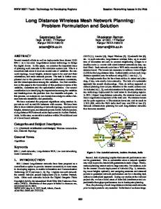
Fig. 1.
Ethernet RJ45
Network model: Adding a node
Previous
New “New node”
Last ”New node”
ACK
ACK
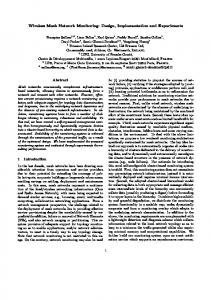
A. Introduction During our research, we focused on the deployment of an indoor WMN with the aid of 802.11 technology. To minimize wireless interference between the links, we chose to use the 802.11a standard, which allowed us to have a multitude of non-interfering channels at our disposal. As with the 802.11g standard, only three orthogonal channels are available. Despite the previous, we noticed that, during our experimental studies, adjacent channel interference is still a major problem in multichannel WMN’s, especially when only a limited frequency spectrum is available, as is the case with 802.11g [8] [9]. Often, this problem is underestimated when planning practical set-ups. During an intervention, a rescue team enters a building, and, to maintain connectivity, regularly deploys new nodes. Because of the nature of this procedure, the network will have a relaying character. We assume that each node has a maximum of two wireless interfaces. Based on this scenario, the dynamic channel selection algorithm, assigns channels to each link, in such way that, for each node the uplink and downlink connections are configured at different channels. To reduce interference between non-adjacent links, each newly deployed node will scan the environment and will assign a channel that is not yet in use, to one of its interfaces. The other interface is set to the default channel, as seen in Figure 1. While the underlying character of the network is a mesh topology, due to channel assignment, a relaying network is created. To dynamically assign the channels when a new node is deployed, several messages are exchanged. In Figure 2,
Last node
Default channel WLAN radio Ad-hoc Wifi
Switch to channel X Channel switch
Channel switch
ACK Resume OLSR
Resume OLSR
ACK
ACK
Fig. 2.
Packet flow
a schematic overview of the messages that are exchanged between the last but one (previous), the last, and the new node is shown. B. Design considerations By design, our planning tool will assure the relaying architecture of the deployed WMN. Our goal is to maintain a high quality link between the intervention team and the outside world, during the exploration of the building. Intuitively, the rescue team is not able to carry a huge number of nodes. Therefore our target is to deploy an extensive and redundant network, with a limited amount of resources. To achieve this, we deliberately choose, when dropping a new node, to not only guarantee a high broadband connection with the previous node, but also to assure at least a low bandwidth connection with the penultimate node. With this approach low rate data communication is still possible, e.g. voice, in case of a node failure.
III. ROUTING PROTOCOL A. Introduction The routing protocol we use in our WMN is the Optimized Link State Routing (OLSR) [10] because if its pro-active, table-driven nature. The protocol utilizes a technique call multipoint relaying to flood messages throughout the entire network. All nodes in the WMN maintain a consistent and upto-date view of the network. Each node broadcasts HELLOmessages to inform its neighbors about its presence. When the network topology changes, the nodes disperse update messages throughout the network to preserve an up-to-date network topology view. For our monitoring tool, each node must have a correct overview of the complete network, to be able to make an end-to-end path capacity estimation. Moreover, OLSR and our monitoring tool, are transparent to the underlying link layer. B. Optimized link state routing Basically, two types of control messages are used in OLSR to exchange topology information: HELLO-messages and Topology Control(TC) messages. The former are periodically broadcast between neighbor nodes locally. These messages are used to maintain an up-to-date view of the status of links between neighbors. The TC messages have a larger scope and are used to spread link-state information throughout the network. The information in the TC messages provides each node with an overview of the whole network. The operation of diffusing a message throughout the network, called flooding, is optimized in OLSR by MPR-flooding. IV. P LANNING THE NETWORK To assist the fire fighters in the deployment of the nodes while they penetrate the building, the planning tool will continuously monitor the signal strength between the surveillance team and the last deployed node in the mesh network. As the reconnaissance team (RT) moves further inside the building, the signal strength will drop, and as soon as it drops below a certain threshold, the team member will be alerted to deploy a new node. In order to guarantee the necessary connectivity, we conducted a series of experiments to determine this threshold. We chose the threshold in such a way that not only the last but also the last but one node can be reached with a decent signal quality. As our aim is to provide a broadband connection with the outside world, the network must be resilient enough to maintain a VoIP connection, even in the case of a node failure. As a consequence of our channel selection protocol, our last node can only measure the signal strength of packets sent by the last but one node, which is tuned to the same channel. It is therefore very important that the aforementioned threshold is wisely chosen. The lack of absolute values for the current signal strength or even of the noise floor in 802.11, forces us to make use of RSSI (Received Signal Strength Indicator) values, which can be retrieved from the driver. When using Atheros cards, these RSSI values can be mapped to dBm values [11]. During our experiments, we set
up a direct 802.11 link between two nodes. To eliminate external wireless interference, we installed the nodes on a Qosmotec test platform [12]. This test platform consists of two large shielded boxes. Each wireless interface of our nodes is connected directly to the Air Interface Simulator of the test platform by means of a coax cable. This platform allows us to attenuate to the wireless signal in a controlled manner and to eliminate external interference. We measured the RSSI of incoming packets at one node while we increased the attenuation of the wireless signal, staying conform to the free space path loss propagation model, as shown in Figure 3. Simultaneously, we measured the UDP throughput over a link with the IPerf tool. Figure 4 shows the measured RSSI versus the throughput. The figure suggests that, for CM9 cards using the 801.11a standard, when the RSSI value drops below -70 dBm, the throughput rapidly decreases from 32 Mbps UDP to zero. For 802.11g, the throughput also significantly drops when RSSI goes below -70 dBm, however, it remains stable at 7Mbps, even when RSSI decreases further, up to the point when the RSSI value drops below -87 dBm. The reason for this phenomenon is that a wireless adapter configured to use 802.11g can switch to 802.11b when signal becomes too weak to sustain a connection. The 802.11b standard uses a different modulation technique than 802.11g and 802.11a, namely DSSS rather than OFDM. As low data rates can be selected in 802.11b, better results can be achieved at low signal strength, compared to 802.11a and 802.11g [13]. Note that the exact values of RSSI measurements differ with each distinct type of wireless cards. From our experiments we concluded that -70 dBm is a good choice for the threshold used to determine the moment the intervention team needs to deploy a new node; this in the specific case where 802.11a and CM9 cards are used. However, to ensure connectivity with the penultimate node, we account for a margin of 7% or 5 dBm. Hence, we fix our threshold to -65 dBm. Knowing that each time the signal strength decreases with 3dbm the quality of the signal halves, according to our propagation model, we can reason that even in a worst case scenario 68 dBm is received at the penultimate node. This is still 2 dBm above our determined threshold. This guarantees a good link quality from the last node to the last but one node. To take possible fluctuations in the measured signal into account we use a sliding window. If the RSSI value drops a predefined number of times below the aforementioned threshold in a given window, a new node must be deployed. V. M ONITORING THE NETWORK During rescue interventions, it is essential that the monitoring tool rapidly gives up-to-date information about the network state, without injecting too much overhead. Most of the endto-end probing techniques, suffer from slow convergence. Bandwidth estimation techniques on a per hop basis lack the end-to-end overview in the network, which is very interesting in WMNs. Our technique combines the best of two approaches: endto-end capacity estimations can be obtained based on per-hop
Topology: --------
22 M
---------------
bit/s Topology: --------
M t/s bi
Topology: --------
---------------
7 Mb it/s
18
10 Mbit/s
---------------
Packet pair probing OLSR Topology: ----------------------
Fig. 5.
Fig. 3.
RSSI vs attenuation
Fig. 4.
RSSI vs throughput
measurements, even under rapidly changing network conditions. Moreover, measurement overhead is kept to a minimum. The next section explains the monitoring mechanism, while Section V-B comments on test results obtained in controlled and real life environments.
Monitoring the network
nel information is disseminated throughout the network, by means of the existing OLSR messages. As OLSR is proactive and table-driven, each node has knowledge of the whole topology of the mesh network. The link capacity and channel information of each node on a path can be used to identify the bottleneck-link and to make an end-to-end bandwidth estimation of that path. Figure 5 visualizes the distributed monitoring concept. We assume that links that are configured to operate on different channels, do not interfere with each other. Furthermore, in our bandwidth estimation model, we assume that each two links on the same channel only interfere if they are less than k-hops positioned from each other. Parameter k must be configured according to the density of the network. In the considered scenario a good value for k is 3. When we want to make an estimation of the path capacity between two hops in the network, the channel capacity will be calculated for each channel that is used by one or more links on the path. Denote the channel capacity for channel x as Cx = Lp /Tx , where Lp is the probe packet length and Tx is the time to transmit the packet over the subset with size hx of all links on path P that are set to channel x. Now, let C(i,x) be the capacity Lp of link i, i = 1..hx set to channel x. Then, C(i,x) = T(i,x) , and Cx can be written as follows: Cx =
A. Monitoring Mechanism Since we need a procedure that enables us to monitor and measure the state of the mesh network we chose to extend the OLSR routing protocol. Each node estimates the link capacity to each of its neighbors by sending packet pair probes. Two back-to-back packets are sent to each neighbor. The first packet is small and acts as a trigger; it is directly followed by a larger probe packet with size Lp . The time difference between the arrival of both packets is measured and communicated back to the sending node. The minimum of a definite amount of samples is considered to be a adequate estimation of the link capacity. This technique is used because of its responsiveness and minimal intrusiveness on the network. It should be noted that packet pair probing is not always very accurate, since it ignores certain factors that affect the packet delivery time. The link capacity to each of a node’s neighbor that is measured by packet pair probing, together with link chan-
Lp hx !
i=0
From (1) we can denote: Cx =
T(i,x)
1 hx !
i=0
(1)
(2)
1/C(i,x)
Thus, if we calculate for each channel on a path the channel capacity, we can make an estimation of the end-toend bandwidth by taking the minimum of the Cx , which is the bottleneck. Remark that the technique being described, does not take into account several other factors that can influence the path capacity in a WMN, e.g. cross talk between wireless interfaces, adjacent channel interference, . . . The value for parameter k, can also influence the estimated path capacity. More experiments and set-ups are needed to determine the impact.
TABLE I PACKET PAIR PROBING VS I PERF ( A - BAND ) rate auto 54M 48M 36M 24M
iperf 31.30 30.20 31.00 26.50 19.00
pp-probing 27,26 26,60 23.95 20.21 16.50
rate
iperf
pp-probing
18M 12M 9M 6M
14.40 9.89 7.79 5.25
12.38 9.41 7.52 5.25
TABLE II PACKET PAIR PROBING VS I PERF ( G - BAND )
Fig. 6.
Packet pair probing in 802.11a
rate auto 54M 48M 36M 24M 18M 12M
iperf 31.10 29.50 31.80 25.20 18.20 13.70 9.70
pp-probing 29.78 28.72 26.35 22.75 16.76 13.28 9.66
B. Measurements and Experimental Verification
VI. C ONCLUSION In this paper, we have proposed a planning tool that aids a rescue team in deploying a wireless mesh network. To offer a real-time overview of the status of the network, we have
iperf
pp-probing
9M 6M 11M 5.5M 2M 1M
7.30 4.99 7.91 4.2 1.78 0.90
7.49 5.33 8.04 4.85 1.78 0.90
Iperf vs. Monitoring Tool
16 Measured Application Layer Datarate (Mbps)
While evaluating single hop packet pair probing over a wireless 802.11a link, we noticed an accurate and stable behavior in the results at lower data rates. However, at higher data rates, we observed a high fluctuation in the results. This is shown in Figure 6. We suspect that this behavior is caused by the fact that our probe packets are queued in the driver. During the tests, no background traffic was generated and the experiments were performed in a shielded environment. If we take the average of the values for a certain period, packet pair probing gives a good indication of the link capacity, as can be seen in Table I and II. Notice that for high data rates, packet pair probing has the tendency to underestimate the link capacity. Although we were able to achieve acceptable results with this technique it needs to be further optimized, e.g. retransmissions, RSSI, data rates could be considered. Therefore, layer 2 optimizations are needed. Outside the shielded environment, tests were performed in a two-hop scenario. The results in Figure 7 show the end-toend throughput estimation together with Iperf reference results. During the test, the first hop was set at a fixed rate of 18 Mbps, while the second hop link was set at a non interfering channel with a varying link rate starting from 6 Mbps to 18 Mbps. The figure shows large similarities between the estimation and Iperf results, indicating that the developed tool provides reliable estimations. Note that a big advantage of using the packet pair probing based estimation tool, is that it imposes very low overhead on the network. In addition, it is hardly influenced by other traffic that is simultaneously sent over the network. Thus, the tool can be used as a background process, providing capacity information about the network, without posing too much overhead on the network.
rate
14
IPERF Monitoring Tool
12 10 8 6 4 2 0 6
9 12 Link Datarate (Mbps)
Fig. 7.
18
Multi-hop monitoring
described and implemented a distributed monitoring tool based on existing probing techniques. We have performed measurements on a real testbed, and showed, by analysis of the results, that a good status of the network can be obtained with our monitoring tool. We also discussed some practical problems that we experienced during our experiments. Future research can focus on optimizing the used techniques and measuring available end-to-end bandwidth by cross-layer concepts. Extending our method to be used in larger and denser wireless mesh networks, is subject for further study. ACKNOWLEDGMENT This research is partly funded by the Flemish Interdisciplinary institute for Broadband Technology (IBBT) through the Geobips project and the Institute for the Promotion of Innovation through Science and Technology in Flanders (IWTVlaanderen). R EFERENCES [1] S. Bouckaert, J. Bergs, D. Naudts, et al., “A mobile crisis management system for emergency services: from concept to field test,” Proceedings
[2] [3]
[4] [5] [6] [7] [8] [9] [10]
[11]
[12] [13]
(on CD-ROM) of the WiMeshNets06 workshop, the First International Workshop on. I. F. Akyildiz, X. Wang, and W. Wang, “Wireless mesh networks: a survey.” Computer Networks, vol. 47, no. 4, pp. 445–487, 2005. R. Draves, J. Padhye, and B. Zill, “Routing in multi-radio, multi-hop wireless mesh networks,” in MobiCom ’04: Proceedings of the 10th annual international conference on Mobile computing and networking. New York, NY, USA: ACM Press, 2004, pp. 114–128. Z. Yang, C. Chereddi, and H. Luo, “Bandwidth measurement in wireless mesh networks.” [Online]. Available: http://www.hserus.net/ cck/pubs/bw-mesh.pdf C. Dovrolis, P. Ramanathan, and D. Moore, “Packet-dispersion techniques and a capacity-estimation methodology,” IEEE/ACM Trans. Netw., vol. 12, no. 6, pp. 963–977, 2004. L.-J. C. Tony, “Adhoc probe: Path capacity probing in wireless ad hoc networks.” [Online]. Available: citeseer.ist.psu.edu/734658.html J. P. Sharad, “Estimation of link interference in static multi-hop wireless networks.” [Online]. Available: citeseer.ist.psu.edu/742631.html C. Chaudet, D. Dhoutaut, and I. G. Lassous, “Performance issues with ieee 802.11 in ad hoc networking,” IEEE Communications Magazine, pp. 110–115, July 2005. Chen-Mou Cheng, Pai-Hsiang Hsiao, H. T. Kung, Dario Vlah, ”‘Adjacent Channel Interference in Dual-radio 802.11a Nodes and Its Impact on Multi-hop Networking”’ T. Clausen, P. Jacquet, C. Adjih, A. Laouiti, P. Minet, P. Muhlethaler, A. Qayyum, and L.Viennot, “Optimized link state routing protocol (olsr),” Internet Engineering Task Force, RFC Experimental 3626, October 2003. J. Bardwell, “You believe you understand what you think i said: The truth about 802.11 signal and noise metrics,” 2004. [Online]. Available: http://www.connect802.com/download/techpubs/2004/ you believe D100201.pdf Qosmotec, “Qosmotec software solutions,” http://www.qosmotec.com. M. S. Gast, M. Loukides, Ed. Sebastopol, “802.11 Wireless Networks: The Definitive Guide“, CA, USA: O’Reilly & Associates, Inc., 2002.