AAS 14-335 COLLISION AVOIDANCE MANEUVER OPTIMIZATION

AAS 14-335

COLLISION AVOIDANCE MANEUVER OPTIMIZATION Claudio Bombardelli∗, Javier Hernando Ayuso†, Ricardo García Pelayo‡ The paper presents a high accuracy fully analytical formulation to compute the miss distance and collision probability of two approaching objects following an impulsive collision avoidance maneuver. The formulation hinges on a linear relation between the applied impulse and the objects relative motion in the b-plane, which allows to formulate the maneuver optimization problem as an eigenvalue problem. The optimization criterion consists of minimizing the maneuver cost in terms of delta-V magnitude in order to either maximize collision miss distance or to minimize Gaussian collision probability. The algorithm, whose accuracy is verified in representative mission scenarios, can be employed for collision avoidance maneuver planning with reduced computational cost when compared to fully numerical algorithms.

INTRODUCTION The continuous growth of the space objects population in Earth orbit can in principle be stabilized by preventing massive space objects such as satellites and rocket bodies from colliding with each other. While for derelict objects this can only be done by physically removing them from crowded orbital regions (whenever that will be technologically feasible) when at least one of the two objects has the capability to modify its own orbit a collision avoidance maneuver (COLA) is possible and is routinely conducted whenever a predicted conjunction exceeds a collision probability threshold established by the specific satellite operator. While collision COLA maneuvers involve lower fuel expenditures compared to satellite deorbiting/reorbiting operations they are conducted several time during the lifetime of a satellite and their frequency is expected to increase as the number of space debris increase and as ground-based tracking systems improve. It will therefore be paramount to devise high-fidelity and high-efficiency optimization strategies to be embedded into dedicated maneuver planning software tools (see for instance1, 2 ). Typically, these tools perform an optimization analysis to minimize the maneuver cost, measured for example in terms of required delta-V, given a required upper limit for the collision probability with one or more space objects that are predicted to fly closely to the satellite of interest. This optimization process can be very demanding from the computational point of view as in the most general case the orbital motion of the two colliding objects needs to be propagated numerically and starting from a 3-dimensional parameter space for the input variable (direction of the maneuver impulse in space and maneuver location along the orbit). One fundamental aspect of this complex optimization process is the modeling of the relative dynamics of the two objects. Recent advances in this regard have been made by one of these authors,3 ∗

Research Fellow, Space Dynamics Group, Technical University of Madrid (UPM), Madrid, Spain Graduate student, Space Dynamics Group, Technical University of Madrid (UPM), Madrid, Spain ‡ Professor, Technical University of Madrid (UPM), Madrid, Spain †

1

who derived an accurate analytical approximation of the b-plane relative motion of two colliding bodies in Keplerian orbits following a generic impulsive avoidance maneuver. That formulation, valid for a generic collision geometry and arbitrary eccentricity, was employed as a base for an optimization process aimed at maximizing the collision miss distance between the two colliding objects for a given magnitude of available delta-V providing interesting and sometimes counterintuitive results. Nevertheless, in order to make the formulation applicable to a realistic scenario three additional steps are needed: 1. Consider collision probability, instead of collision miss distance as the objective function of the optimization problem. 2. Generalize the optimization process to include the case of an initially non-zero miss distance vector at close approach. 3. Analyze the influence of environmental perturbations. The goal of the present work is to tackle these aspects using closed-form analytical expressions and to propose an efficient numerical scheme to solve the optimization problem in its most general form. One crucial advantage of the proposed formulation is the linear dependence between the applied ∆v impulse and the displacement along the collision b-plane. This allows to write the objective function (i.e. the collision miss distance or the collision probability) as a quadratic form eventually reducing the optimization problem to the solution of a simple eigenvalue problem (see Conway4 for a similar result applied to impulsive asteroid deflection) and the solution of a simple non-linear algebraic equation. The article is organized as follows. First we review the computation of the collision probability between two objects given their relative b-plane position and covariance matrices and following the approach presented in reference.5 Next we develop our optimization strategy starting from the linear dynamics formulation of reference3 and addressing the maximum distance and the minimum collision probability problems including the generic case of a predicted b-plane offset before the maneuver. We then apply the proposed method to the 2009 Iridium-Cosmos collision comparing the maximum miss distance with the minimum collision probability scenario. Finally we test the accuracy of the method with a numerical model including the perturbing acceleration of the J2 gravitational harmonic. COLLISION PROBABILITY Let us consider two objects S1 and S2 experiencing a conjunction event with an expected closest approach relative position re . Let us assume that a collision would take place whenever the following condition is verified: krk = kr1 − r2 k < sA , where r1 and r2 are the randomly distributed positions of S1 and S2 and sA can be taken as the sum of the radii of the spherical envelopes centered at S1 and S2 , respectively. The probability of collision between S1 and S2 can be written, in general terms, as the triple integral of the probability distribution function fr (r) of the relative position of S1 with respect to S2 over the volume V swept by sphere of radius sA centered at S2 :

2

Z fr (r) dr.

P =

(1)

V

When the statistical distribution fr (r) is Gaussian it can be written as:   exp − 21 (r − re )T C−1 r (r − re ) fr (r) = , p (2π)3/2 det (Cr )

(2)

where Cr is the covariance matrix of r, which corresponds to the sum of the individual covariance matrices of r1 and r2 , expressed in the same orthonormal base, when the two quantities are statistically independent. When the temporal extent of the conjunction is small compared to the orbit period of the objects one can consider the motion of the two objects of S1 and S2 as uniform rectilinear with deterministically known velocities v1 and v2 , and compute the collision probability as a two-dimensional integral on the collision b-plane. To this end we define the S2 -centered b-plane reference system < ξ, η, ζ > as in6 and with: uξ =

v2 × v1 , kv2 × v1 k

uη =

v1 − v 2 , kv1 − v2 k

uζ = uξ × uη .

Under the rectilinear approximation V becomes a cylinder along the η axis and Eq. 1 can now be written in < ξ, η, ζ > axes and integrated for −∞ < η < +∞ to yield:

) #, ( "   
1 ζ − ζe 2 (ζ − ζe ) (ξ − ξe ) ξ − ξe 2 2 q dξdζ + − 2ρξζ 2 1 − ρξζ P = exp − σξ σζ σζ σξ A 2πσξ σζ 1 − ρ2 ξζ (3) where re = (ξe , 0, ζe )T is the expected closest approach relative position in b-plane axes, A is a circular domain of radius sA and σξ , σζ , ρξζ can be extracted from the relative position covariance matrix in b-plane axes whose (ξ, ζ) minor reads: Z

" Cξζ =

σξ2 ρξζ σξ σζ

ρξζ σξ σζ σζ2

# .

Using Chan’s approach (see5 for details) the computation of Eq (3) can be made equivalent to integrating a properly scaled isotropic Gaussian distribution function over an elliptical cross-section. If the latter is approximated as a circular cross-section of equal area the final computation of the impact probability reduces to a Rician integral that can be computed with the convergent series:

P (u, v) = e−v/2

∞ X vm 2m m!

m=0

with:

3

m X uk −u/2 1−e 2k k! k=0

! (4)

s2 qA σξ σζ 1 − ρ2ξζ

u=

 v=

2

ξe σξ

 +

ζe σζ

(5)

2 − 2ρξζ

ξe ζe . σξ σζ

(6)

From the above equations it appears that the collision probability is constant when the impact point (ξe , ζe ) belongs to an ellipse of semi-axes ratio σξ /σζ and rotated by an angle: 2ρξζ σξ σζ σξ2 − σζ2

1 Θ = tan−1 2

! .

In addition, the collision probability decreases exponentially for increasing v, i.e. as the size of the ellipse increases. MANEUVER OPTIMIZATION In this section, the optimum direction for an impulsive collision avoidance maneuver for minimizing collision probability is computed. The optimization is based on a linear relation derived in reference3 between the b-plane impact point displacement and the applied maneuver impulse. After recalling the previous relation we analyze the optimum maneuver maximizing the collision missdistance before considering the collision probability minimization problem. The two problems are compared. Finally we generalize the optimization for the case of no direct impact (ξe , ζe 6= 0). Collision avoidance dynamics Following reference3 let us suppose a direct collision (ξe = ζe = 0) is predicted when the maneuverable satellite S1 has orbital true anomaly θc , radial orbital distance Rc and eccentricity e0 . Let the velocity of S2 at collision be related to the velocity of S1 by a (positive) rotation of by an angle −π < φ < π around the S1 orbital plane normal uh1 : φ = atan2 [(v1 × v2 ) · uh1 , v1 · v2 ] ,

(7)

followed by an out-of-plane rotation −π/2 < ψ < π/2 in the direction approaching uh1 : " −1

ψ = tan

# (v2 · uh ) kv2 × uh k , v22 − (v2 · uh )2

(8)

and by rescaling its magnitude (v1 ) by a factor χ = v2 /v1 . The resulting b-plane shift ∆r = (∆ξ, ∆η, ∆ζ) after the maneuver impulse ∆v = (∆vr , ∆vθ , ∆vh ) performed at an angular distance ∆θ = θc −θm from the expected collision obeys the linear relation: ∆r = RKD∆v = M∆v where:

4

(9)



 0 0 −1 R =  cos β − sin β 0  , − sin β − cos β 0      K=   

−

√ v1 µ Rc

sin α sin θc

0

− √cos α sin2 φ cos ψ 2

√

sin ψ 1−cos2 ψ cos2 φ

cos α sin φ 1−cos2 ψ cos2 φ

√

1−cos ψ cos φ

√

0

s D=



0

sin φ cos ψ 1−cos2 ψ cos2 φ

    ,   

  c ctθ 0 Rc3  tr crr crθ 0  . µ 0 0 cwh

In the above equations β represents the angle between v1 and vrel and obeys: cos β = p

1 − χ cos ψ cos φ 1 − 2χ cos ψ cos φ + χ2

,

sin β =

p 1 − cos2 β,

(10)

µ is the Earth gravitational constant and α is the flight path angle of S1 at collision, which obeys: e0 sin θc sin α = p 2 ; e0 + 2e0 cos θc + 1

1 cos α = p 2 . e0 + 2e0 cos θc + 1

Finally the terms ctr , ctθ , crr ,crθ ,cwh are non-dimensional functions of e0 , θc and θm provided in reference.3 For the the singular case corresponding to cos ψ cos φ = ±1 the matrix K yields:     K0 =   

−

√ v1 µ Rc

sin α sin θc 0

0

− cos α

0

cos α



   . 1    1

Maximum miss distance maneuver The maximum miss distance optimization problem corresponds to finding the direction of the applied impulse ∆v impulse, with |∆v| ≤ ∆v0 , that maximizes the distance of the b-plane intersection of S1 from the b-plane origin and can be formulated as: maximize Jr (∆v) = ∆ξ 2 + ∆ζ 2 subject to f (∆v) = ∆vT ∆v − ∆v02 ≤ 0

(11)

Jr can be written as: Jr = ∆rT Q∆r,

5

(12)

with: 

 1 0 0 Q =  0 0 0 , 0 0 1

(13)

Jr = ∆vT MT QM∆v = ∆vT A∆v.

(14)

and by use of Eq. 9:

The optimization problem can now be conveniently solved with the method of Lagrange multipliers. After introducing the Lagrangian function: L (∆v, λ) = Jr − λf

(15)

the necessary conditions for the existence of a maximum obey: ∂L = 2A∆v − 2λ∆v = 0, ∂∆v which is an eigenvalue problem. After a quick inspection it can be shown that: ( rank (A) =

for θc − θm = 2πn

1

2

otherwise

(16)

,

meaning that there is always at least one impulse direction leaving the collision unaffected. When two non-zero eigenvalues are present the optimal solution is associated with the maximum eigenvalue λ1 with the corresponding unit eigenvector s1 providing the direction of the optimal impulse: ∆vopt = ∆v0 s1 and the corresponding maximum miss distance: ∆rmax =

p λ1 ∆v0 .

Note that for the direct-hit case analyzed here the maximum distance can be obtained with both a positive and negative ∆v0 impulse along the s1 direction. Minimum collision probability maneuver The minimum collision probability optimization problem can be formulated as:     ∆ξ 2 ∆ζ 2 ∆ξ ∆ζ maximize JP (∆v) = + + 2ρξζ σξ σζ σξ σζ T

subject to f (∆v) = ∆v ∆v −

∆v02

Jδ can be written as: JP = ∆rT Q∗ ∆r,

6

≤0

(17)

with:   Q∗ =  

1 σξ2

0

ρξζ σξ σζ

0

0 0

0

ρξζ σξ σζ

1 σζ2

  . 

and by use of Eq. 9: JP = ∆vT MT Q∗ M∆v = ∆vT A∗ ∆v. Similarly to the previous case the optimization problem reduces to calculate the eigenvalues and eigenvectors of A∗ . The eigenvector s∗1 associated to the maximum eigenvalue λ∗1 provides the direction of the optimal impulse for minimum collision probability: ∗ ∆vopt = ∆v0 s∗1 ,

and the corresponding minimum collision probability can be computed by substituting: vmax =

p λ∗1 ∆v0

into Eq. 4. Non-direct impact In this section the general case of a non-direct impact is analyzed. Since it has been shown that the maximum miss distance and minimum collision probability are formally equivalent, we will refer to the first case. When the impact is non-direct (re 6= 0) Eq. 9 is generalized to: ∆r = re + M∆v

(18)

The corresponding squared miss distance (Eqs.(12,13,14)) becomes: Jr = (re + M∆v)T Q (re + M∆v) = rTe Qre + ∆vT A∆v + 2rTe QM∆v.

(19)

After dropping the constant term rTe Qre and multiplying by ∆v0 the objective function the optimization problem can be conveniently rewritten as: maximize J˜r (u) = uT Au + 2bT u subject to f (u) = uT u − 1 ≤ 0 where we set: u = ∆v/∆v0 ,

7

,

(20)

bT = rTe QM/∆v0 . The problem is a non-convex quadratic optimization problem , which can be reduced to the following convex problem:7


2
2 sT1 b sT2 b minimize + +λ , λ − λ1 λ − λ2 subject to λ ≥ λ1

(21)

where λ1 , λ2 and s1 , s2 are the two non-zero eigenvalues of A, in descending order, and the corresponding eigenvectors, respectively. Eq. (21) leads to the condition:  2  T 2  sT1 b s2 b  + −1=0 , λ − λ1 λ − λ2   λ ≥ λ1

(22)

which can be easily solved with Newton’s method providing λopt . Once λ has been determined the corresponding ∆v can be obtained as:7 ∆vopt = −∆v0 (A − λopt I)† b,

(23)

where the dagger sign represents the pseudo-inversion matrix operation. The maximum miss distance is finally obtained by substituting Eq.(23) into Eq.(19). NUMERICAL CASE To illustrate the results of our optimization we consider a hypothetical collision avoidance maneuver prior to the 2009 Cosmos-Iridium collision. The encounter geometry is summarized in Table 1. In addition we assume an 4 m spherical envelope for the Cosmos 2251 (due to its 6.5 m boom) and a 3 m envelope for Iridium 33 providing sA = 7 m. We then assume, for both objects, a diagonal covariance matrix with standard deviation of 1 km in the along-track and 100m in both the normal and cross track directions∗ . Employing the formulas of the Appendix for the covariance matrices summation we obtain:  Cξζ =

0.02 km2 0 0 0.80 km2

 .

Finally, we assume that a non-direct impact is expected with ξe =0 and ζe =100 m. A 10 cm/s ∆v maneuver is applied at an angular distance ∆θ from the conjunction location. The radial, transversal and out-of-plane components of the impulse can be conveniently written as: ∗

These values are freely chosen as a numerical example and do not represent the actual situation at the time of the collision

8

Table 1. Iridium-Cosmos encounter geometry. Here Iridium is the maneuverable satellite (S1 ).

a0 (km)

e0

φ(deg)

ψ(deg)

θc (deg)

χ

7155.8

2 × 10−4

180.0

77.5

-16.85

1.0

∆vr = ∆v cos γ sin (σ + α)

∆vθ = ∆v cos γ cos (σ + α)

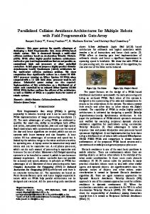
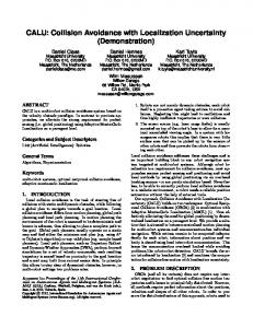
∆vh = ∆v sin γ where α is the flight path angle, σ is the in-plane rotation, opposite to the orbit angular momentum direction, of the maneuver velocity vector with respect to tangent to the orbit, and γ is the subsequent rotation along the out-of-plane direction (see3 ). A fully tangential impulse corresponds to σ = γ = 0. Comparison between minimum-collision-probability and maximum-miss-distance maneuver Figures (1-3) compare the optimal maneuver orientation angles and the b-plane trajectory for varying ∆θ in the case of minimum collision probability and maximum miss distance. Both the angles and the b-plane trajectory look quite different when ∆θ is small while they tend to converge to the same value as ∆θ → ∞. The difference for small ∆θ are due to the fact that the b-plane relative position ellipse is very elongated in the direction of the ζ axis so that a maneuver strategy minimizing collision probability tends to shift the b-plane position towards the ellipse edge rather than to get the farthest away from the center of the b-plane, as it occurs when miss distance is maximized. Note that in the limit case in which σζ → σξ the ellipse would become a circle and the two optimization problems would become equivalent. Notably, there appear to be deep local minima in the collision probability curve which are not so pronounced in the miss distance one. This suggests that when collision probability has to be minimized the satellite operator should perform the maneuver near very specific “favorable” orbital position to get the maximum benefit. Furthermore there appear to be no relation between the collision miss distance local maxima and the collision probability local minima.

9

180

10

P

min

160

rmax

140

0 −10

100

γ (deg)

σ (deg)

120

80 60 40

−30 −40

20

Pmin

−50

0 −20

−20

π

2π

3π ∆ θ (rad)

4π

5π

−60

6π

rmax π

2π

3π ∆ θ (rad)

4π

5π

6π

Figure 1. Optimal in-plane (left) and out-of-plane (right) maneuver orientation angles for the Cosmos-Iridium 10 cm/s COLA maneuver. −3

10

4000

Collision probability

2500 2000 1500 1000

−5

10

−6

10

−7

10

Pmin

500

rmax π

2π

3π ∆ θ (rad)

4π

5π

−8

6π

10

π

2π

3π ∆ θ (rad)

4π

5π

Figure 2. Miss distance (left) and collision probability (right) comparison for the Cosmos-Iridium 10 cm/s COLA maneuver. 1000

Pmin rmax

500 ξ (m)

miss distance (m)

max

−4

10

3000

0

Pmin r

3500

10−5

10−4

0

10−6

−500

−1000 0

500

1000

1500 2000 ζ (m)

2500

3000

Figure 3. Comparison of b-plane crossing point following a 10 cm/s COLA maneuver using minimum probability and maximum miss distance optimization criteria. Collision probability contour lines are drawn for reference.

10

6π

0.25

5000

Keplerian J2

4000 miss distance (m)

error (%)

0.2

0.15

0.1

0.05

0 0

3000

2000

1000

π

2π

3π

4π 5π ∆θ (rad)

6π

7π

8π

0 0

π

2π

3π

4π 5π ∆θ (rad)

6π

7π

8π

Figure 4. Error of the proposed analytical formulation when compared to a high accuracy analytical propagation for the Cosmos-Iridium 10 cm/s COLA maneuver. The collision miss distance is shown on the right for reference.

ACCURACY OF THE METHOD As mentioned earlier, the proposed formulation considers Keplerian orbits and neglects environmental perturbations. The approach is justified by the fact that the COLA maneuver causes a relatively small deviation (relative to its orbital distance) of the maneuvered satellite path compared to its original trajectory. The effect of any perturbing acceleration is proportional to such displacement and scales as the acceleration gradient which is orders of magnitudes smaller than the main gravity gradient even for the dominant perturbation in the densely populated part of the LEO environment: the J2 effect. The error associated to the J2 effect has been investigated numerically and compared to small intrinsic error of the analytical model already proposed in Ref.3 To this end each orbit has been propagated backward from the conjunction orbital state (at θc ) up to the maneuver point (θm ) including the J2 perturbation and then propagated forward with after applying the optimized ∆v impulse (again with the J2 perturbation active) up to the collision point to finally compute the numerically accurate miss distance. Figures (4,5) show the error associated with a J2-perturbed and a Keplerian numerically propagated orbit for the Iridium-Cosmos collision case and for a near head-on collision. An inclination of 86 degrees has been employed for the maneuverable satellite (Iridium) of the former case. The near head-on collision differs from the former case by the angle ψ, set to 1 degree, and by the inclination of the maneuverable satellite (45 degrees). While the Iridium-Cosmos collision shows negligible error (