Abilities and Capabilities of Regression and Decision Trees for ...
Recommend Documents
trees to study Dutch diminutive allomorphy, while Eddington and ...... XIE Huayang, Peter ANDRAE, Mengjie ZHANG & Paul WARREN. In: HOGAN J., P.
Gustavo A Valencia-Zapata, Juan C Salazar-Uribe, Ph.D. Escuela de .... 2002 2.016. Total. 5027 2022 7049. TABLA V. CHI-SQUARE TEST. Value. Exact Sig.
Trade creditors / Total liabilities. Tctl. Activity. +. Trade debtors / Total assets. Tdta. Activity. +. Nepierian logarithm total assets. Ln_asset. Size. +/-. Total assets.
sents a major milestone in the evolution of artificial intelligence, machine ... overfit the training data and encourage profoundly misleading conclusions (Einhorn, ... evaluating the predictive performance of every tree in the pruning sequence on in
Statistical analysis was carried out using XLSTAT 2010 trial version software. .... because the method allows the ready integration of qualitative data, we tested ...
of Soil Reaction in DobrovÄÅ£ Basin (Eastern Romania) ... Romanian Academy, Department of IaÅi, Geography Group, 8 Carol I, 700505, IaÅi (Romania), email:.
{dsim,sj}@cs.umb.edu. ABSTRACT. We introduce an extension of the notion of ..... ing Repository. The ÑйÑÐÑ tree builder from the ÑЧÐ1ÑoÐ package has been ...
comprehension, coding speed, and automotive and shop. We use ..... Evidence from School-Entry Laws,â Journal of Human
Guiso, David Laibson, seminar participants at the 2010 AEA meetings, Household Financial Decision ...... Sanjay Deshmukh
Feb 14, 2015 - [7] G. Coquillard, B. Palao, and B. K. Patterson, âQuantification .... [35] P. Karakitsos, A. Pouliakis, C. Meristoudis et al., âA preliminary study of ...
Afonso, G. Battaglia, D. Seck, G. Le Teuff, et al. To cite this version: C. Quantin, Lynne Billard, M. Touati, N. Andreu, Y. Cotin, et al.. Classification and Regression.
Michelangelo Ceci, Annalisa Appice, Donato Malerba. {ceci, appice ..... SMOTI REG. Av. MSE. M5'. Av. MSE. M5'. Pruning. Av. MSE. Abalone. 4.483. 3.91. 2.59.
drivers and the DR DOS kernel into upper memory. In my case I ... DR DOS has a CACHE com- mand which establishes a ... from MS-DOS. Very large parti-.
Nov 6, 2009 - try to fit models locally and then paste them together, but again they can be ... 1We could instead fit, s
Nov 6, 2009 - node in the tree, we apply a test to one of the inputs, say Xi. Depending on the outcome of the test, we g
Leo BREIMA'/, Jer(,me H. FRIEDMAN, Richard. A. OLSHEN ;,nd Cb.arles J. STONE. ('lassilicatioll and Recession Trees. The Wadsworth Statistics/Probabilit~.
The data come from an experiment (Moolgavkar, Luebeck, de Gunst, Port ..... value h = 0:3, our method yields the logistic regression tree in Figure 5. It has ..... Suresh Moolgavkar of Fred Hutchinson Cancer Research Center for their help in.
producing what we call kernel regression trees. ...... IOS Press. Breiman,L. (1996) ... In Proceedings of the 8th International Conference on Machine. Learning.
sion. Chipman et al [11] recently performed an extensive comparison of several ... The authors would like to thank Daniel Fink, Wes. Hochachka, Steve Kelling ...
Feb 15, 2002 - software program that is designed to evaluate radiographic and clinical features of ... the hands-free documentation process, but such systems are not yet ..... instance of homecare telemedicine, patient edu- cation, and online ...
[9]. Let be a measure of the âgoodnessâ of a candidate split s at node , where. (1) .... 71.91 9. Laptop. 27.66 65. Server. 0.43. 1. Total. 7.46. 235. Node 4. Nominal.
Previous algorithms for constructing regression tree models for longitudinal ... In a different direction, Yu and Lambert (1999) treat each longitudinal data vector ...
Department of Computer Science and Engineering. University of North ...... received the BS degree in Computer Science from Beihang. University, China, in ...
split is pure if after the split, for all branches, all the data taking a ... pure and we have zero training error. ... our framework for autonomic failure management in a.
Abilities and Capabilities of Regression and Decision Trees for ...
all the Representatives in the US House of Representatives of the year 1984. ... The Representatives themselves are ordered by state (and alphabetically.
ITM Web of Conferences 14, 00009 (2017) APMOD 2016
DOI: 10.1051/itmconf/20171400009
Shaking the trees: Abilities and Capabilities of Regression and Decision Trees for Political Science Christoph Waldhauser1 , and Ronald Hochreiter2 , 1 2
KDSS Data Science, 1060 Vienna, Austria. WU Vienna University of Economics and Business, Welthandelsplatz 1, 1020 Vienna, Austria.
Abstract. When committing to quantitative political science, a researcher has a wealth of methods to choose from. In this paper we compare the established method of analyzing roll call data using W-NOMINATE scores to a data-driven supervised machine learning method: Regression and Decision Trees (RDTs). To do this, we defined two scenarios, one pertaining to an analytical goal, the other being aimed at predicting unknown voting behavior. The suitability of both methods is measured in the dimensions of consistency, tolerance towards misspecification, prediction quality and overall variability. We find that RDTs are at least as suitable as the established method, at lower computational expense and are more forgiving with respect to misspecification.
1 Introduction Roll call voting behavior of legislators in the US Congress is at the focal point of many political science research efforts. A traditional model relies on W-NOMINATE scores to condense the many roll call records into a small number of dimensions. We offer a different approach, using a supervised machine learning method that is of equal potency. We test this using two different scenarios, one pertaining to analytical questions of where a vote can be located at in the political sphere. The other scenario relates to predicting how the other legislators will vote, using only a small number of “declared” or “known” legislators. This paper is organized as follows. First general observations regarding the suitability of machine learning methods in political science are being discussed. There, we focus on both the popularity of these methods in general and the contrasted methods in particular, as well as on caveats specific to applications in voting studies. We then turn the reader’s attention on the methods compared in this paper. We put special emphasis on using them in both predictive and analytic roles. We then introduce the testing methodology to set a fixed set of scenarios in which both methods are to be used and explain the indicators employed to ascertain a method’s suitability. The next section describes the results obtained from applying the methods to the scenarios outlined before. Finally, we discuss these results and offer some concluding remarks. e-mail: [email protected] e-mail: [email protected]
ITM Web of Conferences 14, 00009 (2017) APMOD 2016
DOI: 10.1051/itmconf/20171400009
2 Machine Learning and Voting Studies As outlined above, this paper is about applying a premier machine learning algorithm to the study of voting behavior in the US House of Representatives. These applications have a rather long history in engineering and computer science, as they are considered difficult problems. This history is so profound, that there is even a voting data set contained in the wealth of the UCI machine learning repository: the 1984 Congressional Votes Records Database [1]. That data set contains the voting behavior of all the members of the 1984 US House of Representatives on key decisions of that year. It has been used numerous times over the years in different levels of applications ranging from articles [2–5] to books [6] to PhD theses [7]. Most of these works exhibit some degree of neglect towards the specialties [8, 9] of a political science domain, some even grave mistakes. While this negligence is of little importance in evaluating the quality of machine learning approaches or algorithms, it is crucial for assessing a method’s usability in political science. It is only after the peculiarities of the political science domain have been taken into consideration and molded into an algorithm, that the practitioner can successfully wield the tool. The 1984 Congressional Voting Records Database is a data set that details the voting behavior of all the Representatives in the US House of Representatives of the year 1984. The items that are listed, are 16 key votes, as they were singled out by the Congressional Quarterly Almanac of 1985 [10]. While the CQA identifies nine different voting behaviors, in the data set, the variables are recoded into three-valued categorical variables. Additionally, party membership of the Representatives is coded as a dichotomous variable. The Representatives themselves are ordered by state (and alphabetically thereafter), thus generating an inherent structure to the data set, that is neither described nor accounted for. While [11, p. 85] argue that 1984 was a pretty normal year regarding party influence on the Representatives, the specifics of the data set make it rather cumbersome to use in the evaluation of party affiliation prediction algorithms. We will now examine the conceptual shortcomings of the data set in detail. Representatives in the US Congress can take different actions when a bill hits the floor. Obviously, they can vote yea and nay. They can also declare how they would have voted, if they had been present. And they can abstain from a vote. “The CQA lists nine different types of votes: voted for, paired for, and announced for (these three simplified to yea), voted against, paired against, and announced against (these three simplified to nay), voted present, voted present to avoid conflict of interest, and did not vote or otherwise make a position known (these three simplified to an unknown disposition).”(from the data set description as provided by [1]). These simplifications in the data set are not uncontested. The CQA print version, for instance does not follow this simplification, but rather just denotes the pure Yeas and Nays. While the details of the nature of the vote may have some significance for democratic transparency, it does not change the outcome of a vote. If a majority votes Yea, announces or pairs for a motion, the motion is being accepted. For the pure assessment of the outcome of a vote a detailed modeling of the vote’s nature is not necessary. However, if it is not only the outcome that is interesting, but the voting behavior itself, a lot of information is discarded by following the simplifications of the data set. 2.1 Voting Data considerations regarding missing values
Voting behavior data, or more precisely, roll call votes of the US Congress as used here, are records of votes cast by legislators. These votes can be either in the affirmative of or against a proposed piece of legislation. However, there is a third kind of vote besides the more expressive Yea and Nay:
2
ITM Web of Conferences 14, 00009 (2017) APMOD 2016
DOI: 10.1051/itmconf/20171400009
abstention. One approach is to consider abstentions as some sort of missing value: a legislator that did not find the time to cast a vote. We shall now consider the effects of assuming abstentions to be simply missing values. Missing values are instances of a variable that do not have a reliable data point associated with them. The traditional text-book example would be a missing response from a questionnaire, or an obviously failing gauge in a more technical setting. The treatment of traditional missing values has been discussed in length in literature, [5], as a more recent example, suggest one of the following methods to deal with missing values: “A simple solution involves ignoring instances and/or attributes containing missing values, but the waste of data may be considerable and incomplete data sets may lead to biased statistical analyses. Another alternative is to substitute the missing values by a constant. However, it assumes that all missing values represent the same value, leading to considerable distortions. The substitution by the mean/mode value is common and sometimes can even lead to reasonable results. However, this approach does not take into account the between-attribute relationships, which are usually explored by data mining methods. Therefore, a more interesting approach involves trying to fill missing values by preserving such relationships.”[5, pp. 245] They continue detailing their approach, and evaluate it using the CQA data set. There, they count “435 instances, of which 203 have missing values. These instances were removed (to make the prediction evaluation possible) and the proposed method was employed in the remaining ones”[5, p. 251]. The authors thus did exactly what they were warned not to do in the data set description. While it is certainly possible to think of not cast votes as simply missing values, because the Representatives did either not have an opinion on a subject, or did not find the time to come to Congress, this model appears presumptuous if applied to key votes. Key votes, by definition, are important to the parties in Congress, and possibly to the nation at large. It is difficult to imagine that a Representative would simply not find the time to vote for a key subject. Furthermore, given the importance of the vote and hence the strict party discipline enforced by party leadership, it is highly unlikely that a Representative that did really not have an opinion on a subject, did not vote, and thus risk disciplinary measures by his or her own party leadership, just because she did not have an opinion. It is much more likely, that Representatives did vote only present because their constituents wishes were against the party line, they however did not want to risk their party standing by voting against the party line. To sum up, the modeling of not cast votes as missing values does not adequately reflect the nature of these votes. While it is clearly not possible to ascertain the motivation behind a not cast vote, discarding it entirely results in the discarding of potentially valuable information. Obviously, the replacement of an unknown vote with a mean or median value is equally flawed, if party affiliation prediction is the goal. We therefore argue to include the not cast votes into the analysis, by changing the binary variable (with missings) to a ternary one (without missings). In terms of level of measurement this would yield a qualitative factor variable on a nominal scale with three factor levels: nay, yea and present. There, however, is more information included in this variable. Nay, yea and present are not only distinctive categories or types of votes, they also contribute to an outcome, that is to the passing or rejecting of a proposed law. Either party that wishes to see a law passing Congress, will have to ensure that the majority of the valid votes (i.e. without the present votes) are yea votes. In that sense, yea votes not only present a category, but a category that is of greater value than a nay or present vote. This is to say that there is an inherent ordered structure in these values. We can thus elevate the level of measurement to ordinal scale.
3
ITM Web of Conferences 14, 00009 (2017) APMOD 2016
DOI: 10.1051/itmconf/20171400009
Another interesting property of these variables is the actual weight of a vote. Clearly a yea vote is as supporting of the passing of a law as a nay vote is damaging. Since every vote is equally capable of determining the outcome, they posses the same weight. Hence, the distance between yea and nay votes on a line is the same. Similarly, present votes do not favor either side. They merely reduce the number of valid votes, and this benefits both sides struggling to further their respective causes. So changing the interpretation of the variables from neutral voting behavior to supporting the motion and thus implementing a numeric coding of −1 for Nay, 0 for present, and 1 for Yea, allows an interval scale level interpretation of the voting variables. This has profound consequences, as interval scaled variables provide access to a large number of statistical methods, that would have been out of the question otherwise. For the scope of this paper, we use the terms 2-value logic to refer to the coding of abstaining as a missing value. Using the information of abstention on the other hand leads to a 3-value logic model. Another major flaw in the data set is the coding of party affiliation. While certainly Representatives of the 98th US Congress all belonged to either the Republicans or the Democrats, this only partly mirrors reality. Owing to a newly found strength and to thus resulting motivation, the Republicans managed to find some sort of coherence in their voting behavior in the 1980s. The Democrats, however, were made up of two quite distinct parties, that shared little more than a common name and party leadership. The case of the Democrats is widely recognized in political science literature [12, 13], yielding even CQA to break down democratic votes into Southerners and Northerners. The data set does not follow this tradition: Southern and Northern Democrats alike are coded as Democrats and Democrats only. However, we will not dive any deeper into this issue here, as the CQA data set is mainly of historic value, and we will here use a more up-to-date collection of votes. 2.2 Overfitting avoidance
Many machine learning tools excel at prediction. The here introduced method of RDTs falls in the so called class of supervised learners. This means that an algorithm is trained on predicting by showing it already predicted data. For instance, when the algorithm should be trained to recognize apples, it needs to shown different objects, some of them apples and some of any other type. It will then deduce the criteria that turn an apple into an apple. This then can be used to classify other objects where we do not yet know if it is an apple or not. The first set with identified objects is called the training set. The test set is then the collection of cases that are to be predicted. However, when predicting, one must take care to strike a balance between a model that explains the data very well, but then cannot predict formerly unseen objects. For instance, the apple identification task might lead to a model that learned that every round object is an apple, and will therefore wrongly classify oranges as apples. To avoid this, it is best practice to repeat the training many times, to get an idea of how dependent the algorithm is on certain features. If there is fear that the algorithm wrongly overemphasizes certain features, an averaging or bagging approach like random forests can be used. These averaging approaches, however, are not a topic we will discuss here any further. Instead, we focus on estimating the variance between different training runs. This is done by randomly splitting the data set into two parts: a training and a test set. These parts are then used for training and testing the prediction quality. This is repeated many times, with each time the case allocation to a training or testing role is varied randomly. This gives many prediction results, that then can be compared to arrive at an idea of the variance. If this variance is low, as it is in this case as we will see shortly, the no bagging is needed. As we are dealing with roll call data here, it is worth noting that varying the random trainingtesting set approach is quite easy to implement. Another approach would be to use roll call data from a previous session. While this is in theory possible, it would be very difficult to accomplish in practice.
4
ITM Web of Conferences 14, 00009 (2017) APMOD 2016
DOI: 10.1051/itmconf/20171400009
Table 1. Decision/Classification/Regression Trees as method in journal articles.
Journal American Political Science Review American Journal of Political Science Public Opinion Quarterly
–2007 9 10 1
2008–2012 0 0 2
Table 2. W-NOMINATE scores as predictors in journal articles.
Journal American Political Science Review American Journal of Political Science Public Opinion Quarterly
–2007 6 7 0
2008–2012 1 2 0
This would require that the roll call records of the testing period be somehow linked with those of the training period. Returning to the apple example: if the algorithm was trained on classifying objects because of their color and shape, but then is tested on the information of weight only, it will fail. Only if we could somehow deduce a link between color/shape and weight, could the algorithm be successfully applied. When resorting to the splitting of a single data set, these limitations do not apply. 2.3 Literature review
As noted above, the concept of regression and decision trees is not new. It’s heyday in political science use, RDTs enjoyed right after their invention in the 1980s. In the following, we would like to give an overview of the literature relating to RDT applications in political science’ three premier journals: American Political Science Review, American Journal of Political Science and Public Opinion Quarterly. These journals have been chosen as they have been continuously ranked as the journals with the highest impact factor in political science by Thomson Reuters Journal Performance Indicators. The following Table 1 gives an overview of articles using RDTs as a method in those journals1 Additionally, the use of W-NOMINATE scores as predictors in regressions was researched. These results2 are found in Table 2. The periods have been broken down in two discrete areas, revolving around a split point in 2008. Especially with decision trees, there is a wealth of articles referring to qualitatively established decision trees, that are, however, unrelated to the here discussed methodology (e.g. [20]). Therefore, these articles have been removed. As was demonstrated in this section, thought needs to be given to way voting data is being represented. These choices have serious consequences to the toolbox being available to modelers. As apparently the popularity of RDTs in social sciences has somewhat faded, we will now turn our attention towards the methods contrasted in this paper: regression and decision trees and W-NOMINATE based models.
3 Regression and Decision Trees Regression and Decision Tree Analysis differs greatly from the formerly discussed regression analysis. While regression analysis starts with a statistical model, and tries to adjust its parameters to fit the 1 The most recent articles using data driven RDTs are [14, 15]. [16] is one of the first texts of using data driven methods in social sciences, and takes a very critical stance. 2 The most recent articles containing W-NOMINATE as content of regression models are [17–19].
5
ITM Web of Conferences 14, 00009 (2017) APMOD 2016
DOI: 10.1051/itmconf/20171400009
model to the data, RDTA goes the same way backwards: its starting point is located within the dataset. From there the data is divided, or grouped along its variables, with the goal to create as pure groups as possible. To this end, the variables have to be rank ordered for their suitability of splitting and a split value has to be determined. Another problem with RDTs is that they can grow quite large. Therefore, a technique called pruning is employed, after the tree has grown, to eliminate all portions of the tree that are not important for the final result. Important here means contributing actively to the quality of the classification. For this some sort of purity measurement (i.e. how good does a node apply to only one of the groups) has to be developed. RDTs can be used for a variety of tasks. One of the more common applications is the classification of data into different groups. [21] term decision trees that classify along a discrete feature classification trees, while trees that produce a clustering with variable membership rates are labeled regression trees. For the aim of this paper, we will combine both tree species under the term RDTs. The central questions that need theoretical foundation in a RDTA “pertain to the criteria for splitting nodes and pruning the tree” [21, p. 270]. The former is a measure of divisibility as mentioned above, while the latter assess how complex a tree has become and how useful a node can be, purity. Splitting is rather straight forward, but unfortunately it is computationally unfeasible to try out all possible splits, and then prune the useless ones. So usually a greedy algorithm is used for growing the initial tree. For pruning that tree, a plethora of interestingness measures has been proposed in the literature. As one of the most important purity measures, and highly recommended by [21], the Gini index will be used in this paper. For the two classes case, the Gini index is defined as GI = 2p(1 − p), with p being the proportion in the second class. The lower the GI for a node, the purer it is, and the more information can be won from keeping the split (and possibly its successive branches) in the tree. Pruning is repeated for all of the nodes in the tree, and yields an optimal result. Of course, if the initial split got flawed by some means, pruning cannot help anymore. So due care must be payed by choosing the initial variable for the split. A possibility is, to not just randomly pick it, i.e. start the search at a random point, but to start from a variable that is rather pure itself. Within R, the function rpart() provides the necessary functionality to grow and prune a tree. It provides different approaches in growing the tree that are suitable for classification tasks or for instance to group survival analysis data or to grow regression trees. The function is complemented by a plotting utility that produces dendograms of the grown trees. The default plotting capabilities are extended by [22]. A grown tree can then be used to predict the outcome for unseen cases. By examining a new cases values at the splitting nodes of the tree, the case is moved further down the tree until it finally arrives at a leave node that then assigns that case its predicted value.
4 W-NOMINATE Scores An entirely different approach to the analysis of voting behavior is pursued by W-NOMINATE scores, as introduced by [23]. Here, a three-step multidimensional scaling method is applied iteratively to voting data. In essence, the idea behind W-NOMINATE is to reduce the many single vote variables into a few dimensions. So instead of describing a legislator’s voting behavior in terms of hundreds or thousands of recorded votes, this behavior is condensed in some (i.e. less than 10, usually 2) newly created variables with the canonical interpretation of economic and lifestyle based divides. In that, this method is similar to principal component or exploratory factor analysis. W-NOMINATE and its
6
ITM Web of Conferences 14, 00009 (2017) APMOD 2016
DOI: 10.1051/itmconf/20171400009
extension, dynamic W-NOMINATE are de-facto standards for locating US electors in political space. Therefore, we refer the reader to established literature detailing the intricacies of W-NOMINATE. Here, we will now focus on using W-NOMINATE scores to predict voting behavior for legislators whose intentions on a particular vote are not yet clear. To this end, the W-NOMINATE scores (w1 , w2 , . . . ) obtained from the past voting record are used as predictors in a logistic regression, modeling the voting behavior (Yea vs. Nay) for the vote in question:
5 py ln = β0 + βi wi 1 − py i=1
Here βi denotes the regression coefficient for the i-th W-NOMINATE score. To ensure a properly fitting model, step-wise selection is being applied afterwards, to remove those terms that do not contribute to model quality. This model can be used to arrive at a probability of voting yea for unknown legislators, given their past voting record and thus their W-NOMINATE scores. A predicted probability of mode than 0.5 is used to classify that legislator as a future yea-voter; otherwise the legislator will be assigned the class of nay-voter. W-NOMINATE score estimation is implemented by the wnominate package in R [23]. This package, however, is based on FORTRAN code and takes a heavy toll computational wise. For instance, computing the W-NOMINATE scores on the 110th House in 5 dimensions took about 15 minutes on a reasonably sized computer. For comparison, the computation of a decision tree with the same input variables took mere 2 seconds.
5 Testing Methodology To establish the suitability of RDTs for political science applications, we looked at the two distinct tasks. The first task centered on producing an analytically accessible model of voting behavior. The second task was to predict the outcome of key votes, using only prior voting behavior as predictors. We will discuss both tasks in turn now. 5.1 Analyzing voting behavior
A central virtue of any model is to not only fit the data it is based on well. Rather, a model algorithm also needs to produce a model that is transparent in that it allows researchers to interpret the modeling choices made, i.e. a black-box model is always of less value than one from which analytic insights can be deduced. For the analytic scenario, the task was set to provide a model that allows a classification of a vote along arbitrary dimensions. This arbitrary dimension allowance was added for comparability of W-NOMINATE and RDTs. The idea is to be able to call a vote being like another vote or similar to political dimension. For the W-NOMINATE approach, this can be achieved by looking at the regression coefficients produced in the model described above. Since the W-NOMINATE scores are normalized to lie within a unit circle (or hyper sphere for higher dimensions), they can be compared with each other to establish which dimension has the largest influence on a vote. Likewise, in RDTs the tree’s variable selection can be interpreted as votes that are similar to the vote in question. When assessing analytic model qualities, we looked for sensitivity to parametrization with regards to consistency. A different model specification should not lead to a completely different model.
7
ITM Web of Conferences 14, 00009 (2017) APMOD 2016
DOI: 10.1051/itmconf/20171400009
5.2 Predicting voting behavior
For this task the following scenario was assumed. Before a key vote, individual representatives are contacted to inquire on their voting intentions. Additionally, legislators may have chosen to publicly state their intended behavior. Using this knowledge, and assuming that there are no last-minute mood swings in the legislators, the voting behavior of the remaining representatives is to be predicted. As additional predictors, this scenario permits the using of past voting behavior for every elector. Armed with this information, a decision tree can be grown following this formula: Vj
j−1
Vi + P
i=1
Here, V j is the vote to be predicted. The (possible) predictors for this vote is the past voting record for all votes (V1 to V j−1 ) and the representative’s party membership. Comparing the predicted voting behavior of the missing legislators to the the one actually observed later on, a quality measure for the prediction can be established: the proportion of the legislators’ vote that was wrongly classified leads to the misclassification rate. Obviously, the lower the misclassification rate, the better or more accurate the prediction is. A model that is able to successfully predict how legislators will vote, arguably captures the political process in detail. If that model is also able to be analyzed, i.e. is not a black box, scientists can gain insights on correlations between votes, i.e. examine what makes legislators vote the way they do. Further, any such model has useful applications in lobbying industries. In the following, two models were pitted against each other. One model was formulated among more traditional lines: here, a logistic regression model used the W-NOMINATE scores of legislators to predict their voting behavior on a key vote. The W-NOMINATE scores were computed using all the votes in the data set that had occurred before the to-be-predicted vote was cast. The second model uses a decision tree to arrive at the same prediction. As input variables, the algorithm could choose from all previously cast votes. The set of legislators was split randomly into known and unknown legislators. The assignment of each legislator followed a uniform random distribution. Different sizes of training sets were tried out and predictive performances compared. The set of known legislators was used to train, i.e. grow the decision tree or estimate the regression parameters. This tree/model was then used to predict how the unknown legislators would vote. To establish the quality of a prediction, we examined how many legislators’ votes were incorrectly predicted. Putting that number into relation with the total number of legislators to classify, the misclassification rate is computed. To ensure reliability of the obtained misclassification rate, a Monte Carlo technique, namely cross-validation, was used. This means that each classification was repeated many times over, splitting the data set randomly into known and unknown legislators. A useful model, therefore, will be able to predict unknown legislators’ voting behavior comparably accurate. Additionally, it should be able to do so with only few legislators being known. Also, the quality of the prediction should not be dependent on which legislators are known. This means, that not only the misclassification rate has to be low. The successful model also needs to exhibit a low level of variance between the cross-validation replications. A high level of variation would require many models to be computed. Combining these many models to arrive at a meta-model that allows also analytical insight is far from trivial. Low variation eradicates that need. In this section we have stated two scenarios that can be used to answer questions in the field of political science. Further, indicators have been identified that allow judging a method’s suitability. The analytical scenario requires to provide consistency even in the face of misspecification, while in
8
ITM Web of Conferences 14, 00009 (2017) APMOD 2016
DOI: 10.1051/itmconf/20171400009
the predictive scenario it is important to produce accurate predictions with a low variability. We will now apply both methods in both scenarios to data from the 110th US House, describing the obtained results.
6 Results In the following we present the results using the aforementioned methodology on a specific set of voting data. The data set analyzed was that of the first session of the 110th US House of Representatives, as provided by [24]. This data set contains all the roll call votes of all Members at that time. The data set has 449 rows (legislators, some of them came into office or left office during the time covered) and 1865 columns (recorded roll call votes). Each field has one of 3 possible values, representing yea, nay and abstained. A number of votes have been identified as key votes by the editors of the Congressional Quarterly weekly reports. These votes were selected because they got wide media coverage, or controversial or particularly close. They can also be a test of presidential power. Key votes as identified by CQ have been used regularly in political science [25, 26]. To test the advantages of RDTs over the traditional W-NOMINATE-based regression, a random stretch of votes, namely Votes 200–250 were selected. Additionally, more in-depth analysis was conducted on a randomly selected key vote: 836. 6.1 Analysis
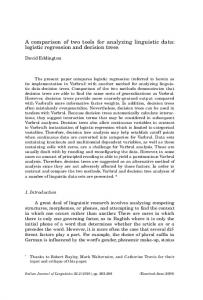
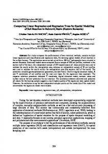
To gauge analytical model qualities, the entire data set of roll call votes was used to explain a singled-out key vote. To do that, both approaches were provided with either a 2-valued or 3-valued parametrization as detailed above. In the following, the estimated logistic regression parameters and effect plots for the resulting W-NOMINATE based models will be contrasted. After that, the regression and decision trees produced will be presented. As stated above, a key value of any model is insensitivity to different ways of parametrization. One possibility to judge this quality is by looking at the models produced using a 2- and a 3-valued specification of voting behavior: does the consideration of abstainers alter the resulting model? When computing W-NOMINATE-based models, the step-wise feature selection algorithm is forced to remove the third component from 2-value model. As a result, the coefficients of both models vary strongly. One efficient way to render these differences are the effect plots that are given in Figure 1. These effect plots detail, that both models lead to similar effects of most W-NOMINATE score dimensions. However, dimension three is removed from the 2-value model and dimension five has a much milder effect in the 2-value model than in its 3-valued brother. While the ultimate conclusion, that Vote 836 is a vote that can be explained well along the first W-NOMINATE dimension is not altered, the effect sizes between model specifications do vary considerably. Tasking RDT-based models with producing analyzable models leads to dendograms of the respective trees. They are depicted in Figure 2. While both model parametrizations lead to similar choices in splitting points, the finer-grained model results in a more detailed tree. However, there are no contradictions. 6.2 Prediction
For the task of prediction, both approaches were asked to predict the voting behavior of a majority of legislators for a given vote. As source of information, the past voting behavior of all legislators and the voting behavior of a subset of legislators on the vote in question was provided. The main quantity of interest here is the misclassification rate as defined above. First, the performance of both methods given a different number of known legislators as a training set was compared.
9
ITM Web of Conferences 14, 00009 (2017) APMOD 2016
DOI: 10.1051/itmconf/20171400009
−1.0
−0.5
0.0
0.5
1.0
0.8 0.0
0.2
0.4
0.6
0.8 0.6 0.4 0.2 0.0
0.0
0.2
0.4
0.6
0.8
1.0
Coord 3D
1.0
Coord 2D
1.0
Coord 1D
−1.0
0.0
0.5
1.0
1.0 0.8 −0.5
0.0
0.5
1.0
−0.5
0.0
0.5
1.0
2 value
0.6 0.4 0.2 −1.0
−1.0
Differences 2, 3 value logic
3 value
0.0
0.4 0.0
0.2
0.6
1.0
Coord 5D
0.8
Coord 4D
−0.5
−1.0
−0.5
0.0
0.5
1.0
Figure 1. Comparing the effects of the respective W-NOMINATE-based models parametrized with 2- and 3value logic respectively. If the choice of parametrization is irrelevant, the effect curves should be identical.
These comparisons were done on a randomly selected key vote. The procedure of randomly selecting a given share of legislators as training set was repeated 250 times to produce results indicative of variability. The performances were compared using one-sided two-sample t-tests with the null hypothesis that WNR-based mean misclassification rates are lower (or equal) than those produced by RDTs. The level of significance has been adapted for multiple testing using Bonferroni correction. These results are shown in Figures 3 and 4. It is striking to see the performance differences between the two approaches. While WNR produces a constant quality so to speak, RDTs improve vastly, once a threshold number of legislators used in the prediction is exceeded. What’s more, is also that RDTs exhibit a drastically lower vari-
10
ITM Web of Conferences 14, 00009 (2017) APMOD 2016
DOI: 10.1051/itmconf/20171400009
2 value
3 value
Vote.835 < −0.5 no
yes
yes
Vote.695 = N
N
Vote.832 < 0.5
Vote.835 = N no
Vote.695 < 0.5
Y
Vote.33 < 0.5
0.54
Y
Vote.661 < 0.5
Vote.555 < 0.5
−0.47 −0.99
0.39 −0.22
0.97 0
Figure 2. Contrasting decision trees grown from 2-value and 3-value logic models.
ance across replications. This behavior of low variance and thresholds is also present in all the other key votes, as demonstrated in Figure 5. Note that, due to WNR’s computational expense, no computations for all key votes were carried out for the WNR method. Albeit key votes are arguably the most interesting ones to predict, both methods were also tested using a randomly selected stretch of consecutive roll call votes. The task was again to predict the voting behavior of unknown legislators using only prior voting record as predictors. Each computation was repeated 25 times using different randomly generated training and testing set splits. A series of ttests was computed to test the alternative hypothesis that RDT’s misclassification rate was lower than the one generated by W-NOMINATE based prediction models. The p-values of the resulting tests are
11
ITM Web of Conferences 14, 00009 (2017) APMOD 2016
0.25 0.20 0.15 0.10 0.05 0.00
Mean misclassification rate expression(bar(m))
0.30
DOI: 10.1051/itmconf/20171400009
20
40
60
80
100
Number of known legislators
Figure 3. Comparing prediction performance for WNR and RDTs across different training set sizes for key vote 836. The bottom line is the mean misclassification rate of RDTs, the top line that of WNR-based prediction models. The shaded area are 95% confidence bands. Mean and variance has been established through crossvalidation random sub-sampling with 250 replications.
given in Table 3. When applying a Bonferroni corrected level of significance of 0.001, 12 votes were predicted significantly more accurately using RDTs than using W-NOMINATE.
7 Discussion When comparing methods used for an analytic purpose, the consistency of the model across (inadvertently) chosen parametrizations is a striking factor. The effects resulting from different modeling
12
ITM Web of Conferences 14, 00009 (2017) APMOD 2016
0.10 0.00
0.05
p−value
0.15
0.20
DOI: 10.1051/itmconf/20171400009
20
40
60
80
100
Number of known legislators
Figure 4. P-values for one-sided two-sample t-tests, testing the alternative hypothesis that m ¯ RDT < m ¯ WNR for different numbers of known legislators. The dashed horizontal line indicates the Bonferroni corrected level of significance (0.0026316). Every p-value below that line indicates a significantly better performance of RDTs compared to WNR-based models.
choices in the W-NOMINATE based models, indicate that consistency here is limited. Especially in the higher, and arguably less important dimensions, the observed effects between a 2-value and a 3-value logic differ. Especially noteworthy is the omission of the third dimension from the model specified by a 2-value logic. The RDTs are somewhat similar in this respect. While the 3-valued model results in a superset of the votes selected to describe the 2-value model, there are no contradictions. However, the larger tree allows for finer grained classifications.
13
100
60
100
20
60
100
Vote 284 0.0 0.2 0.4
0.0 0.2 0.4 20
Vote 265 0.0 0.2 0.4
Vote 18
Misclassification rate
60
DOI: 10.1051/itmconf/20171400009
Misclassification rate
20
Misclassification rate
0.0 0.2 0.4
Vote 9
20
60
100
Vote 836
Vote 982
20
60
100
0.0 0.2 0.4 20
60
100
20
60
100
0.0 0.2 0.4
Vote 534
Misclassification rate
Vote 377
0.0 0.2 0.4
Number of known legislators
Misclassification rate
Number of known legislators
Misclassification rate
Number of known legislators
0.0 0.2 0.4
Number of known legislators
20
60
100
Vote 1060
Vote 1118
20
60
100
0.0 0.2 0.4 20
60
100
20
60
100
0.0 0.2 0.4
Vote 1057
Misclassification rate
Vote 1040
0.0 0.2 0.4
Number of known legislators
Misclassification rate
Number of known legislators
Misclassification rate
Number of known legislators
0.0 0.2 0.4
Number of known legislators
20
60
100
Vote 1177
Vote 1183
Vote 1186
20
60
100
Number of known legislators
0.0 0.2 0.4 20
60
100
Number of known legislators
20
60
100
Number of known legislators
0.0 0.2 0.4
Vote 1122
Misclassification rate
Number of known legislators
0.0 0.2 0.4
Number of known legislators
Misclassification rate
Number of known legislators
Misclassification rate
Number of known legislators
0.0 0.2 0.4
Misclassification rate
Misclassification rate
Misclassification rate
Misclassification rate
ITM Web of Conferences 14, 00009 (2017) APMOD 2016
20
60
100
Number of known legislators
Figure 5. Performance of RDTs in relation to the number of known legislators the prediction is being based on for all key votes. Horizontal lines indicate votes that were too easy to predict, i.e. most legislators voted in the same way. Computations averaged over 25 replications.
To summarize, for analytic purposes, W-NOMINATE based and RDT based models are on par with each other. Given the computational expense required by W-NOMINATE score estimation, however, RDTs appear to be more suited for data intensive analysis. Turning to predictions, the differences between both methods become more evident. RDTs exhibit consistently a lower variance over cross-validation replications. RDTs apparently require a threshold level of known legislators to be grown from: only then can they deliver accurate predictions of voting behavior. However, this threshold number is rather low being in the range of 15 to 20. Once this threshold is reached, RDTs consistently produce significantly better results than W-NOMINATE
14
ITM Web of Conferences 14, 00009 (2017) APMOD 2016
Table 3. P-values for one-sided two-sample t-tests, testing the alternative hypothesis that m ¯ RDT < m ¯ WNR for a stretch of 50 votes. Missing entries result from W-NOMINATE based models not converging.
based models. This observation holds for key votes. Ordinary, less important votes, however, are somewhat different. Here RDTs still outperform W-NOMINATE based models most of time. On the other hand there are cases where W-NOMINATE delivers better predictions. We conclude from this, that RDTs have certain advantages over W-NOMINATE based models. For one part, they are much faster to compute. Given the wealth of voting data that is now available, this is an advantage that should not be missed and is likely to grow in importance as big data is being gradually introduced to political science. Another key observation is, that they produce transparent models that can be used to gain analytic insights in political processes. While W-NOMINATE also has much wider general applications, W-NOMINATE based regression models are not terribly useful in understanding the relationships of votes. RDTs on the other hand are easily interpreted. Finally, prediction accuracy of RDTs is extremely high and almost always better than that of W-NOMINATE based models. While both methods have their advantages and disadvantages, we find that RDTs are capable tools that should be used more often in the political science community.
References [1] A. Asuncion, D.J. Newman, UCI machine learning repository (2010), "http://archive.ics.uci.edu/ml" [2] K.W. Bauer, S.G. Alsing, K.A. Greene, Neurocomputing 31, 29 (2000) [3] E.H. Han, G. Karypis, V. Kumar, B. Mobasher, Bull. Tech. Committee on Data Eng. 21, 15 (1998) [4] E.R. Hruschka, E.R. Hruschka, N.F.F. Ebecken, Feature Selection by Bayesian Networks, in Advances in Artificial Intelligence, edited by A.Y. Tawfik, S.C. Goodwin (Springer, 2004), Vol. 3060 of Lecture Notes in Artificial Intelligence, pp. 370–379 [5] E.R. Hruschka, E.R. Hruschka, N.F.F. Ebecken, Missing Values Imputation for a Clustering Genetic Algorithm, in Advances in Natural Computation, edited by L. Wang, K. Chen, Y.S. Ong (Springer, 2005), Vol. 3612 of Lecture Notes in Computer Science, pp. 245–254 [6] W. Davies, P. Edwards, Distributed Learning: An Agent-Based Approach to Data-Mining, in Machine Learning-95, edited by D. Gordon (AAAI Press, 1995) [7] M.A. Potter, Ph.D. thesis, George Mason University, Fairfax, Virgina (1997)
15
ITM Web of Conferences 14, 00009 (2017) APMOD 2016
DOI: 10.1051/itmconf/20171400009
[8] J.E. Jackson, The American Political Science Review 65, 451 (1971) [9] J. Clinton, S. Jackman, D. Rivers, American Political Science Review 98, 355 (2004) [10] M. Cohn, ed., Congressional Quarterly Almanac 1984 (Congressional Quarterly, Washington, D. C., 1985) [11] G.L. Hager, J.C. Talbert, Legislative Studies Quarterly 25, 75 (2000) [12] R. Fleisher, The Journal of Politics 55, 327 (1993) [13] M. Thomas, American Journal of Political Science 29, 96 (1985) [14] D.P. Green, H.L. Kern, Public opinion quarterly 76, 491 (2012) [15] G.R. Murray, C. Riley, A. Scime, Public Opinion Quarterly 73, 159 (2009) [16] H.J. Einhorn, Public Opinion Quarterly 36, 367 (1972) [17] J. Richman, American Political Science Review 105, 151 (2011) [18] J.W. Patty, American Journal of Political Science 52, 636 (2008) [19] E.G. Juenke, R.R. Preuhs, American Journal of Political Science 56, 705 (2012) [20] D. Skarbek, American Political Science Review 105, 702 (2011) [21] T. Hastie, R. Tibshirani, J. Friedman, The Elements of Statistical Learning, Springer Series in Statistics (Springer, New York, 2001) [22] S. Milborrow, rpart.plot: plot rpart models. An enhanced version of plot.rpart (2011), http://CRAN.R-project.org/package=rpart.plot [23] K. Poole, J. Lewis, J. Lo, R. Carroll, Journal of Statistical Software 42, 1 (2011) [24] K. Poole, J. Lewis, 110th house roll call data, Published online (2010), http://www.voteview.com/house110.htm [25] S.A. Shull, J.M. Vanderleeuw, Legislative Studies Quarterly pp. 573–582 (1987) [26] J.N. Victor, N. Ringe, Legislative Caucuses as Social Networks in the 110th US House of Representatives, in Networks in Political Science Conference, Cambridge, MA (2008)