Abstract Introduction

SPE 173362-MS High-Resolution 3D Structural Geomechanics Modeling for Hydraulic Fracturing T. Bérard, J. Desroches, Y. Yang, and X. Weng, Schlumberger; and K. Olson, Southwestern Energy

Copyright 2015, Society of Petroleum Engineers This paper was prepared for presentation at the SPE Hydraulic Fracturing Technology Conference held in The Woodlands, Texas, USA, 3–5 February 2015. This paper was selected for presentation by an SPE program committee following review of information contained in an abstract submitted by the author(s). Contents of the paper have not been reviewed by the Society of Petroleum Engineers and are subject to correction by the author(s). The material does not necessarily reflect any position of the Society of Petroleum Engine ers, its officers, or members. Electronic reproduction, distribution, or storage of any part of this paper without the written cons ent of the Society of Petroleum Engineers is prohibited. Permission to reproduce in print is restricted to an abstract of not more than 300 words; illustrations may not be copied. The abstract mus t contain conspicuous acknowledgment of SPE copyright.

Abstract Three-dimensional (3D) geomechanical models built at reservoir scale lack resolution at the well sector scale (e.g., hydraulic fracture scale), at least laterally. One-dimensional (1D) geomechanical models, on the other hand, have log resolution along the wellbore but no penetration away from it—along the fracture length for instance. Combining borehole structural geology based on image data and finite elements (FE) geomechanics, we constructed and calibrated a 3D, high-resolution geomechanical model, including subseismic faults and natural fractures, over a 1,500- × 5,200- × 300-ft3 sector around a vertical pilot and a 3,700-ft lateral in the Fayetteville shale play. Compared to a 1D approach, we obtained a properly equilibrated stress field in 3D space, in which the effect of the structure, combined with that of material anisotropy and heterogeneity, are accounted for. These effects were observed to be significant on the stress field, both laterally and local to the faults and natural fractures. The model was used to derive and map in 3D space a series of geomechanically based attributes potentially indicative of hydraulic fracturing performance and risks, including stress barriers, fracture geometry attributes, near-well tortuosity, and the level of stress anisotropy. An interesting match was observed between some of the derived attributes and fracturing data—near-wellbore pressure drop and overall ease and difficulty to place a treatment— encouraging their use for perforation and stage placement or placement of the next nearby lateral. The model was also used to simulate hydraulic fracturing, taking advantage of such a 3D structural and geomechanical representation. It was shown that the structure and heterogeneity captured by the model had a significant impact on hydraulic fracture final geometry.

Introduction Geomechanical modeling for input to hydraulic fracture (HF) design can be undertaken using either a 1D or 3D approach. 1D geomechanical models have log resolution (e.g., ½-ft resolution) along the wellbore but no penetration away from it—along the fracture length for instance. 3D geomechanical modeling, on the other hand, is most often applied to the analysis of reservoir-scale processes, and reservoir-scale models have cell dimensions typically ranging from 50 to 200 m horizontally. This compares poorly with typical hydraulic fracture lengths or spacing. A tenfold increase in horizontal resolution is at least needed to provide information at a scale relevant to a hydraulic fracturing treatment. Moreover, any 1D approach relies on the following assumptions: 1. 2. 3. 4. 5.

horizontal layering; laterally uniform properties; isotropic or transverse isotropic vertical (TIV), linear elastic behavior; absence of faults or fractures; absence of coupling between layers.

These assumptions are violated, even when propagating a 1D-based stress profile in a 3D geological structure, and some error must result (the magnitude of which is essentially unknown) in structured, heterogeneous, higher-than-TIV anisotropic, nonlinear elastic, faulted, or fractured rock masses (presumably not infrequently). Each and every one of these assumptions

2

SPE 173362-MS

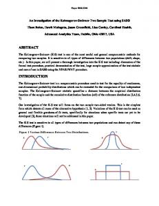
can be relaxed using FE modeling, pending the necessary data are available. Yet data- and workflows are lacking at this intermediate, well sector scale, to document with sufficient resolution the above-listed features away from the well(s), particularly the structure and distribution of rock properties, pore fluid pressures, fractures, or faults. Without them, Occam's razor applies and 1D approaches are sufficient. Seismic data and interpretation traditionally support such characterization away from the well, but, here again, at reservoir scale. We propose a workflow that enables geomechanical modeling in 3D at the scale of a well sector with proper resolution with respect to hydraulic fracturing dimensions. The proposed workflow (Fig. 1) builds on borehole-wall image data and structural geology interpretation and modeling to capture and render the structural setting—faults and natural fractures included—with relatively fine detail, in 3D, up to typically a few hundred meters away from the well(s). The workflow may be performed using well image data only if necessary or may combine image and seismic data. The resulting 3D structural model provides the basis for a 3D FE approach to geomechanical model construction, which allows relaxing the 1D assumptions listed above. The workflow can therefore be expected to deliver an improved geomechanical solution for input to analyses of well-centric processes such as hydraulic fracture design and evaluation, along with wellbore stability, sanding, etc. Such a workflow also helps gradually develop a better understanding of the discrepancy between 1D and 3D stress solutions as a function of the insitu setting and of the impact such a discrepancy may have on the engineering problem at hand. Although a number of applications could potentially benefit from this approach, we concentrate on hydraulic fracture design and evaluation. In this arena, significant efforts have be made in recent years to take into account 3D effects and to develop the corresponding features in the latest generation of hydraulic fracture modeling software (e.g., Kresse et al. 2011, 2012; Weng et al. 2011).

Fig. 1—Overview of the proposed workflow for high-resolution 3D structural geomechanics modeling. We first introduce and illustrate the workflow with an applied case example in the Fayetteville shale play, Arkansas. We then describe in more detail how the geomechanical model was passed as input to hydraulic fracture simulation. We compare the results obtained with the same model, but populated with a 1D-based stress field. Conclusions from that comparison are drawn.

SPE173362-MS

3

Test site dataset A test site, located in the Fayetteville shale play, Arkansas, was identified where a rich dataset was available in a pair of wells comprising a vertical pilot and its associated horizontal, 3,700-ft-long lateral, together with another parallel horizontal lateral. Twenty-eight controlled stimulation experiments were carried out to date on this pair of wells. The layout of the wells is shown in Fig. 2.

5-H 4-H 4-PH Fig. 2—Perspective view of the test site showing the vertical pilot well 4-PH and the two, 2,000-ft-deep, 3,700-ft-long, 650-ft-distant horizontal laterals, 4-H and 5-H. The dataset included a comprehensive suite of logs in the vertical pilot and the two horizontal lateral wells, together with cores and minifrac stress test data in the pilot hole. Summaries of the log data and processed/interpreted results are given in Table 1. Summarized in Table 2 are estimates of both the minimum and maximum horizontal stress magnitudes from MDT* modular formation dynamics minifrac tests (following the method presented in Desroches and Kurkjian 1999). The dataset further included seismic data and seismic interpretation results. However, in view of testing the workflow on well data only, none of it was considered in the present study, except for comparison purposes. Furthermore, in order to test the predictability of the workflow, we decided to use only the data of the pilot hole and the first lateral to generate the entire model for the pair of lateral wells and use the results to forecast hydraulic fracture conditions along the second lateral, as shown later.

4

SPE 173362-MS

Pilot hole (4-PH)

Lateral hole (4-H)

Platform Express* wireline logging tool

Platform Express* wireline logging tool

ECS* elemental capture spectroscopy sonde

ECS* elemental capture spectroscopy sonde

Sonic Scanner* acoustic scanning platform for openhole

Sonic Scanner* acoustic scanning platform for cased hole

Litho Scanner* high-definiton spectroscopy (i.e., StingRay)

Litho Scanner* high-definiton spectroscopy (i.e., StingRay)

OBMI* oil-base microimager / UBI* ultrasonic borehole imager (Pre- and post-MDT)

OBMI* oil-base microimager / UBI* ultrasonic borehole imager (Pre- and post-MDT)

MDT modular formation dynamics tester (dual-packer mode for in-situ stress testing)

Thru-bit log suite (quad combo with shear)

Well log and other data

Whole core (Fayetteville horizon)

Processing / interpretation results Complete petrophysical interpretation UNI and OBMI interpretation

Dip picking, simple DFN

Dip picking, simple DFN

Sonic Scanner interpretation, including mechanical properties and stresses

Openhole

Cased hole, no stress

1D MEM

No

No

Pressures

No (virgin, normal pressures)

No (virgin, normal pressures)

Table 1—Top: Core, wireline log, and test data available in 4-PH (vertical pilot hole), 4-H (lateral), and 5-H (second lateral) wellbores. Bottom: Processed data and interpretation results. Station #

sh (psi)

sh lower bound (psi)

sh upper bound (psi)

sH (psi)

1 2 3 4 5 6 7 8 9

2,510 2,126 1,980 2,350 2,290 1,622 1,725 2,120 2,035

2,440 2,100 1,970 2,260 2,200 1,620 1,720 1,670 2,015

2,520 2,180 1,990 2,508 2,300 1,625 1,740 2,200 2,150

2,604 2,192

sH lower or upper bound status > >

2,390 2,535 2,310

). Empty cells indicate stations where no estimation could be obtained.

Borehole structural geology Structural geology principles provide means for structural modeling in 3D, up to typically a few hundred meters away from the well(s), based on borehole-wall image data only (Etchécopar and Bonnetain 1992; Cheung et al. 2001). In a nutshell, images are processed and structural dips are interpreted along the well. Adjacent dip readings are then grouped into sequences in such a way that all dips within a given sequence are internally consistent with a cylindrical or conical structure. For each such a sequence, a cylindrical or conical structure is best fitted to the corresponding set of dips, which yields the structural parameters of the sequence. Because the structural element associated with each sequence is seen at the well over a certain borehole length, it can be extrapolated away from the well up to a certain distance (typically 1:1). A two-dimensional (2D) illustration is given in Fig. 3. In addition, faults and natural fractures can also be picked on the same images, which enables fault and fracture network modeling.

SPE173362-MS

5

Fig. 3—Illustration of borehole structural analysis and structural reconstruction. The left panel illustrates how bedding planes’ poles picked anywhere within a cylindrical or conical structure align themselves on a so-called great or small circle, respectively, in a stereonet view. The panel in the middle illustrates, on a real case example, how dip readings interpreted on image data are sequenced in such a way that all adjacent dips within a sequence are located along a great or a small circle (or close to it)—i.e., belong to the same structural element. The reconstructed structural elements are shown in a vertical cross section on the right panel with, in this particular example, a tilted layer-cake structure at a relatively shallow depth unconformably overlying a fold at a greater depth. At the test site, both 4-PH (vertical) and 4-H (lateral) wells have oil-base mud imager and ultrasonic borehole imager logs. Image quality ranges from relatively poor to good. These images were processed and interpreted, providing bedding, fault, and natural fracture dip readings. As mentioned earlier, although image data were also acquired in the second lateral (5-H), no data from this well were, on purpose, used in this particular instance. The main steps of the structural model construction are summarized in Fig. 4. Following data quality control (QC) analysis, sequencing of the structural dips was performed interactively. The structural trends were first highlighted using dip vector analyses to guide the structural zonation. Then the raw structural dips were sequenced, filtered, and used to fit the structural elements. Using the well trajectory, formation tops, and structural dips, the true stratigraphic thickness (TST) was computed to help project structural dips vertically. In parallel, three fault planes were created based on image log interpretation. All the above information was finally used to extrapolate the structure away from the wells. Eventually, a structure emerged with four elements separated by these three faults (Fig. 5, top panel). The structural model was observed to be in overall agreement with the structure interpreted independently from the seismic, with yet finer detail captured, including subseismic faults (with throws of a couple tens of feet). A comparison along a vertical section centered on well 4-H is presented on the bottom panel of Fig. 5. Note that seismic interpretation did not resolve any of the faults identified by the structural geology analysis. Image data further provided information on natural fracture orientation and distribution, which enabled discrete fracture network (DFN) modeling (Fig. 6). The overall distribution is relatively scarce. Three fracture sets were identified. Two of them exhibit fault-parallel orientations with higher densities in the vicinity of the faults. They were therefore interpreted as fault-related fracture corridors and modeled accordingly (namely, Fracture Set 1 along Fault 1 and Fracture Set 3 along Fault 3). Even if Fault 2 has a roughly similar orientation as the fractures in Fracture Set 2, there was no spatial correlation between the presence of those fractures and that fault. The structural model, the faults, and the DFN were then passed as input to geomechanical model building, as explained in the next section.

6

SPE 173362-MS

Fig. 4—Main steps of the structural model construction.

Fault 3 Fault 1

Fault 2

Fig. 5—Structural model in a perspective view (top panel). The bottom panel compares, in a vertical cross section along 4-H well, the structure interpreted on image data (colored zonation) and seismic data (black lines). Note that the layering from seismic interpretation ignores the faults, as they were not resolved by it. There is a 3:1 vertical-to-horizontal exaggeration in both panels.

SPE173362-MS

7

Set1

Set3 Set2

Fig. 6—Left panel: Natural fractures and faults observed on images (circle and square symbols, respectively) in an upper hemisphere Schmidt stereoplot, with the three main sets outlined. Right panel: Map view of the modeled DFN (blue patches), faults (lines), and observed fractures along the well (yellow symbols).

Finite Elements geomechanics The building of the geomechanical model involved the following steps. First, the structural grid was refined both horizontally, by considering typical hydraulic fracture length and spacing, and vertically, based on the heterogeneity of observed properties and particularly over the minifrac-tested depth intervals (see Fig. 7, including the table insert comparing the grid size with representative hydraulic fracture dimensions). Further, the grid was expanded by adding some side-, over-, and underburdens in order to mitigate side effects over the volume of interest (Fig. 8). Transverse isotropic elastic rock properties were derived from dipole sonic data, density, and other petrophysical properties. The resulting property profiles were upscaled in and distributed throughout the grid (Fig. 9). Faults and natural fractures were mapped by first identifying the grid cells penetrated by the discontinuities (Fig. 10). Secondly, joints parallel to the local discontinuity orientation were assigned to these grid cells. The properties of the resulting “fractured rock” material, equivalent to the intact rock–joints combination, were solved (Reuss homogenization). Using the compilation published by Hobday and Worthington (2012) as a guideline, the normal stiffness of the faults was set equal to 300,000 psi/ft for Faults 1 and 3 and to 100,000 psi/ft for Fault 2 (the latter was indeed observed to be more compliant on the sonic log data). Following the same guideline, the normal stiffness of the natural fractures was set equal to 600,000 psi/ft. The shear stiffness of the discontinuities was set equal to half the normal stiffness. Note that the presence of these discontinuities results in softer cells than the intact material. A pore fluid pressure field was formed by assuming hydrostatic conditions following a 0.4-psi/ft gradient. A constant pressure was prescribed on the top face of the model equivalent to the weight of the overburden surcharge. The bottom face was set on rollers. Displacement boundary conditions were applied on the lateral faces. The stress field was solved using the VISAGE* FE simulator (Koutsabeloulis and Hope 1998) assuming an elastic behavior for both the intact rock and the

8

SPE 173362-MS

discontinuities. The validity of this assumption was further checked a posteriori, although not presented here. The side boundary conditions were fine-tuned until a satisfactory match was obtained between the modeled and measured stresses (see Table 3 and Fig. 11). Dimensions (ft)

Grid

HF

Thickness / height

5.5 (ave.)

250

Along lateral / spacing

15

60

Perpendicular to lateral / half-length

30

700

Fig. 7—Layering refinement and property upscaling, illustrated along the 4-PH well. Tracks 1 and 2: Initial and refined zonation. Track 3: Cell thickness before and after refinement. Track 4: Depth location of the MDT minifrac tests. Tracks 5– 7: Log and log-upscaled profiles (shown in colored and black lines, respectively) of horizontal Young’s modulus, horizontal Poisson’s ratio, and bulk density. The table in the upper right corner compares the grid size with representative hydraulic fracture dimensions.

Fig. 8—Perspective view showing how the structural model (colored) was embedded by addition of over-, side-, and underburdens (grayed).

9

0.15 0

6

0

Vertical YME (Mpsi)

0.40

0.15

Vertical PR

Horizontal PR 0.40 6

Horizontal YME (Mpsi)

0.3 2.40

2.65

Density (g/cc)

2.3

Shear modulus (Mpsi)

SPE173362-MS

Fig. 9—Vertical cross sections along well 4-H showing bulk density, horizontal and vertical Young’s moduli, shear modulus, and horizontal and vertical Poisson’s ratios.

10

SPE 173362-MS

Fig. 10—Map views showing the grid cells penetrated by the faults and the fractures (top and bottom panels, respectively).

SPE173362-MS

11

4-PH

pp

sh

sH

sV

Azim sh

sH / sh

Fig. 11—Comparison between modeled and measured stresses along 4-PH well. Measured stresses are shown as symbols. Modeled stresses are shown as solid colored lines. Track 1: Zonation. Track 2: Pore fluid pressure. Track 3: Magnitude of the minimum horizontal stress (sh). The best estimates and the lower and upper bounds, from the minifrac tests, are shown as purple, yellow, and black symbols. Track 4: Magnitude of the maximum horizontal stress (sH). The best estimates from the minifrac tests are shown as purple symbols with an indication (shown by the arrow, whenever available) as to whether the best estimate is an upper or lower bound. Track 5: Vertical stress magnitude. Track 6: Azimuth of the minimum horizontal stress. Track 7: Ratio between sH and sh. The best estimates from the minifrac tests are shown as blue symbols with an indication (shown by the arrow, whenever available) as to whether the best estimate is an upper or lower bound.

Table 3—Principal horizontal strains used to prescribe side boundary conditions. To assess the magnitude of the 3D effects on the stress field and therefore evaluate the potential error incurred by neglecting them, a stress field was formed using a typical 1D stress model: Eq. 1 below was used in each and every point of the model to obtain a 1D stress field. It shows minimum and maximum horizontal stresses from the so-called “poro-elastic strain” stress model in TI materials (Thiercelin and Plumb 1994; Savage et al. 1992).Error! Reference source not found.

(1), where: sh = minimum horizontal stress (azimuth taken equal to N140°E) sH = maximum horizontal stress E = horizontal Young’s modulus

12

E’ V V’  sv Pp h H

SPE 173362-MS

= vertical Young’s modulus = horizontal Poisson’s ratio = vertical Poisson’s ratio  Biot coefficient = overburden stress = pore fluid pressure = minimum horizontal strain = maximum horizontal strain

The discrepancy between the 1D and 3D stress fields is shown in Fig. 12 for a layer located toward the middle of the model. The effect of the structure alone (i.e., fault- and fracture-related property alteration excluded, but combined with that of property anisotropy) is seen to be relatively negligible in the present and essentially flat case example. The introduction of faults and fractures as relatively soft discontinuities, however, is seen to significantly perturb the stress field locally. At the faults and fractures and particularly near their tips, this perturbation reaches up to ±1,000 psi in stress magnitude (i.e., ±50%, relative to a background sh magnitude of the order of 2,000 psi), nearly complete horizontal stress rotations (75° or so), and about 50° vertical stress tilt. In the vicinity of the faults and fractures, the stress perturbation is within ±200 psi in stress magnitudes (i.e., ±10%), ±20° in horizontal stress azimuth, and a few-degree stress tilt. Please note that the above figures largely depend on the contrast in elastic properties between the intact rock and the discontinuities.

SPE173362-MS

13

1000

Dsh (psi)

A

DsH (psi)

B

DsV (psi)

C

Dazimuth(sh) (°)

D

-1000 1000

Underestimate by 1D

-1000

1000 Overestimate by 1D

-1000 90

-90 Fig. 12—Map views of the discrepancy between 1D and 3D stress fields. The difference in sh, sH, and sV magnitudes are shown from top to bottom in panels A, B, and C, respectively. The difference in sh azimuth is shown in panel D.

Completion quality mapping Before moving to hydraulic fracture simulation, we present how the geomechanical model can be used to derive and map in 3D space a series of geomechanically based attributes a priori indicative of completion performance and risks, including stress barriers, fracture geometry attributes, near-well tortuosity, and the level of stress anisotropy. Such indicators can be screened in 3D space or along a planned well trajectory to help with well or perforation placement. As an example, these are presented in Fig. 13 along a cross section aligned with the trajectory of well 4-H.

14

SPE 173362-MS

Apart from the general trend in the presence of layers that can act as height growth barriers above the wellbore, and much less below it (until the base of the reservoir is hit, which is known as a strong barrier), lateral variations (along the well trajectory) in the capability of these layers to be a barrier can be observed. Indeed, hydraulic fracturing simulations show height growth variations associated with the 3D stress field, much more than with a simpler 1D stress field (see following section). Strong variations in horizontal stress anisotropy, from 1.05 to 1.4, within the range of that measured by the MDT stress tests can be observed both vertically and along the well trajectory. Similarly, HF simulations reported later in this paper will show a different behavior along the well trajectory. Finally, the effect of faults and natural fractures is clearly seen on the tilt of the stresses, up to 20° in the vicinity of Fault 1. Although never hit by the treatments carried out in this test site, it was expected that treatments in the vicinity of that fault would have been increasingly difficult to complete. Furthermore, to test the relevance of the geomechanical model, potential indicators of near-well tortuosity were computed along the trajectory of well 4-H. In a 3D stress field, the trace of the fracture at the wellbore can be computed, assuming for example that there is pressure communication between the well and the formation (which corresponds to the creation of a pressurized micro-annulus). Because of the presence of the well, that trace will be a different plane than the preferred fracture plane (perpendicular to the minimum principal stress away from the wellbore). Two angles indicative of that trace with respect to the well can be computed ( and  in Fig. 14). However, no correlation was found between those angles and any parameter recorded during the 16 single-stage hydraulic fracturing treatments carried out in that well. Another angle between the initial fracture plane and the preferred fracture plane ( in Fig. 14) can be computed. It was found to very strongly correlate with the near-well tortuosity measured with step-down tests (e.g., Romero and Mack, 1995) on 14 out of the 16 tests. The two other tests not in line with the predicted variation exhibit significantly higher near-well tortuosity. It is proposed that the base tortuosity is associated with the fracture reorientation due to the 3D stress field, on top of which a local tortuosity due to the fabric of the rock (e.g., the presence of calcite rich veins; Burghardt et al., 2015 ) can be added. The prediction of the near-wellbore tortuosity trend in the vicinity of the well’s toe clearly demonstrates that the effect of Fault 3 is captured by our model, providing significant confidence in the model. In order to test the predictive capabilities of our model, we computed various properties along the trajectory of well 5-H, which are presented in Fig. 15: variations of the magnitude of the minimum horizontal stress, the ratio of the two horizontal stresses, and the same angle  described above. The near-wellbore tortuosity also follows the same base trend, apart from two points that are significantly higher, highlighting the predictive capability of the model. The confidence with which the model can be used to forecast hydraulic fracture conditions away from the well used to build the model is therefore strong. Note that the role of local features on the near-well fracture trajectory is clearly demonstrated by the two points around 5,700-ft measured depth (MD), where two distinct calibration treatments were carried out, with one point falling on the trend line and another one significantly higher.

SPE173362-MS

15

A

Upward and downward stress barriers (psi)

Stress anisotropy sH / sh

sV tilt (°)

B

C

D

Fig. 13—Geomechanically based attributes associated with hydraulic fracturing performance and risks in a vertical cross section along 4-H well. From top to bottom: Upward and downward stress barriers, horizontal stress anisotropy, and angle between the vertical and principal stress closest to vertical (stress tilt). There is a 3:1 vertical-to-horizontal exaggeration.

16

SPE 173362-MS

Fracture orientation at the borehole-wall

C

A

Fracture re-orientation between the near- and far-well regions

B

4-18







DPtort. Fig. 14—Profiles along well 4-H of near-well tortuosity indicators. A and B: Schematic illustration of the near-well tortuosity angles used below. On the left side are shown the epsilon and omega angles describing the fracture orientation relative to the well at the borehole wall. B (Abass et al. 1996) illustrates fracture orientation with respect to the well depending on the well orientation with respect to principal stress directions. C: MD, zonation, and well orientation are shown in Tracks 1, 2, and 3. Track 4 shows fracture initiation azimuth relative to top-of-hole (). Track shows the angle between the fracture plane at the borehole wall and the well axis (). Track 6 shows the re-orientation angle of the fracture between the near-well and far-well regions (). The measured near-wellbore pressure drop at 20 BPM for the various hydraulic fracturing treatments is also superimposed to  on Track 6 (DPtort).

SPE173362-MS

17

5-H

Fig. 15—Conditions pertaining to hydraulic fracturing forecast along well 5-18H. Tracks 1, 2, and 3: MD, zonation, and well orientation. Track 4: Minimum horizontal stress magnitude. Track 5: Horizontal stress ratio. Track 6: Re-orientation angle of the fracture between the near-well and far-well regions (labeled “alpha”). The measured near-wellbore pressure drop at 20 BPM for the various hydraulic fracturing treatments is also superimposed to alpha on Track 6.

Hydraulic fracture simulation The geomechanical model (a 3D grid with fault and natural fractures, fully loaded with mechanical properties, fluid pressures, and equilibrated rock stresses) was passed as input to a hydraulic fracture simulator. A complex fracture network model, taking into consideration both the interaction between hydraulic fractures and natural fractures, together with the stress interaction among hydraulic fractures (Weng et al. 2011; Kresse et al. 2011, 2012), is used for the simulation. Fracture simulation was carried out for 4-H well assuming the lateral portion is geometrically divided into eight stages, each consisting of six perforation clusters spaced 80 ft apart. The fracture treatment is simulated using both the 3D geomechanical model and the same model but populated with a 1D stress field from Eq. 1 discussed previously. Both a guar-based cross-

18

SPE 173362-MS

linked gel treatment design and a slickwater treatment design, given in Tables 4 and 5, respectively, are simulated and compared, both for the 1D and the 3D stress models. Stage 1 2 3 4 5 6 7 8 9

Pump rate bpm 65 65 65 65 65 65 65 65 65

Fluid Volume gal 21,000 9,600 30,000 30,000 30,000 30,000 30,000 26,400 24,000

Proppant

40/70 mesh sand 40/70 mesh sand 40/70 mesh sand 40/70 mesh sand 40/70 mesh sand 40/70 mesh sand 40/70 mesh sand 40/70 mesh sand

Proppant concentration lbm/gal 0 0.25 0.5 1 1.5 2 2.5 3 3.5

Table 4—Cross-linked gel treatment pump schedule. Stage 1 2 3 4 5 6 7 8 9 10

Pump rate bpm 100 100 100 100 100 100 100 100 100 100

Fluid Volume gal 32,500 80,000 70,000 30,000 52,500 55,000 58,000 56,000 32,700 6,000

Proppant

100 mesh sand 100 mesh sand 40/70 mesh sand 40/70 mesh sand 40/70 mesh sand 40/70 mesh sand 40/70 mesh sand 40/70 mesh sand 40/70 mesh sand

Proppant concentration lbm/gal 0 0.25 0.5 0.5 0.75 1 1.25 1.5 1.75 2

Table 5—Slickwater treatment pump schedule.

Fig. 16 shows the comparison of the simulated hydraulic fracture geometry for cross-linked gel treatments using 1D and 3D geomechanical models, and Fig. 17 shows similar comparison for the slickwater treatment.

SPE173362-MS

Fig. 16—Simulated fracture geometry and width distribution after 100 minutes of shut-in for all eight stages for crosslinked gel treatment using the 1D geomechanical model (left) and the 3D geomechanical model (right). The light blue lines are the traces of the natural fractures on a horizontal plane cutting through the wellbore.

Fig. 17—Simulated fracture geometry and width distribution after 100 minutes of shut-in for all eight stages for slickwater treatment using the 1D geomechanical model (left) and the 3D geomechanical model (right). The light blue lines are the traces of the natural fractures on a horizontal plane cutting through the wellbore.

19

20

SPE 173362-MS

Several observations are made from the simulation results. The first set of observations highlights the effect of the faults and the natural fractures, regardless of whether the simulations use the 1D or the 3D stress model. The dense natural fractures near Fault 1 cause the fracture wings that intersect these fractures to terminate their growth, as shown in Fig. 18. This suggests that fracture stages near the faults can be strongly affected and compromised. The effect is, however, stronger with the 3D stress model. Let us recall that it is the particular workflow presented here that allowed the faults and the fracture corridors associated with them to be mapped. The second set of observations highlights the effect of the natural fractures and the faults on the stress field, which is captured by the 3D stress model but not by the 1D stress model.  



Compared to the 1D stress model, the stress perturbation caused by the faults and natural fractures captured by the 3D model results in greater variations in the final geometry of the hydraulic fractures along the lateral, as evidenced in Fig. 17. More specifically, the stress perturbation around Fault 3, captured by the 3D stress model and not by the 1D model, strongly affects both cross-linked gel and slickwater treatments. The hydraulic fracture surfaces rotate to be more aligned with the fault and tend to grow toward the lower stress regions near the fault. Furthermore, because of the locally reduced stress near the fault, the fracture width becomes wider there and the fracture extension is thus reduced (e.g., first three stages near the toe in Figs. 16 and 17). Furthermore, that same stress perturbation results in greater variation in the fracture height growth, as shown in Fig. 19.

A third set of observations is linked to the interaction between the various hydraulic fractures in a stage. 

Due to relatively close fracture spacing, there is strong interference among the fractures from adjacent perforation clusters. This results in uneven and asymmetric fracture growth for fractures initiated from different perforation clusters, as evidenced in Fig. 16 and Fig. 17. Two patterns have been observed: o

o



One is an en-echelon pattern, which is observed when the angle of the fracture azimuth and the wellbore axis is relatively small (closer to a longitudinal fracture), in which case the fractures from the perforation clusters near both ends of the stage tend to grow longer while the extension of the fractures from the clusters in the middle is reduced. This occurs more frequently for stages toward the toe in well 4-H because of the presence of Fault 3, which skews the angle of the fracture with respect to the wellbore. The other pattern is in the form of a zipper with every other fracture growing to the opposite side of the well. This is due to the fractures trying to avoid each other to offset the stress shadow and attain wider width (a lower flow resistance state). It tends to occur more frequently when the fracture angle is large relative to the wellbore (closer to a transverse fracture), in this case for the stages at the heel section.

Whether an en-echelon pattern or a zipper pattern occurs also depends on the interplay between stress shadow effect among the fractures and stress anisotropy. Fig. 20 shows the predicted fracture pattern for Stage 8 for cross-linked gel and slickwater using the 3D stress model. For the same stage, the cross-linked gel treatment creates an enechelon pattern while the slickwater creates a zipper pattern. This difference is likely because the net pressure is much greater when a cross-linked fluid is used, resulting in stronger stress interference among the fractures. For the same given stress anisotropy (which acts against fracture turning), that stress interference results in a greater tendency for the fractures to turn.

SPE173362-MS

Fig. 18—Simulated fractures for cross-linked treatment of Stage 6 using the 1D model (left) and the 3D model (right).

Fig. 19— Simulated fractures for cross-linked treatment of Stage 7 using the 1D model (left) and the 3D model (right). Local stress perturbations in the 3D model due to the faults and natural fractures cause variations in the local vertical stress profile, resulting in greater variation in fracture height growth.

21

22

SPE 173362-MS

Fig. 20—Simulated fractures for cross-linked treatment (left) and slickwater treatment (right) for Stage 8 using the 3D model.

Conclusions A workflow was developed for single-well and yet 3D geomechanical modeling. By combining borehole structural geology modeling based on image data and FE geomechanical modeling, the workflow enables the construction of a 3D, structurally involved, and relatively high-resolution geomechanical model at the scale of a well sector—forming proper input to hydraulic fracture model design and evaluation, among other potential applications. The workflow was assembled and tested on a site located in the Fayetteville shale play, Arkansas, where a rich dataset was available, including images, elastic properties profiles, and minifrac stress test data, in a pair of wells comprising a vertical pilot and a horizontal, 3,700-ft-long lateral. Data were used from the pilot hole and its associated lateral only to allow for a blind test of the resulting geomechanical models on the second lateral. No stumbling block could be identified preventing the completion of data- and workflows. With respect to the conventional 1D approach to mechanical earth model (MEM) building, the proposed workflow obviously is more demanding, as both image data and expertise in structural geology and FE are required. It is also more time-consuming, with the geological and geomechanical modeling tasks adding an estimated 2 to 3 weeks. Software integration proved convenient. The use of displacement boundary conditions, compared to stress boundary conditions, yielded equally satisfying results at a much lower cost in terms of model construction and run time. High-enough resolution could be achieved within reasonable run times on a personal computer. Some of the finer (log) resolution is nonetheless shaved, while upscaling and layering deserves proper attention. The workflow was expected, and indeed shown, to provide a better geomechanical solution compared to the one obtained from a 1D approach. First, such an approach is internally consistent, honoring equilibrium conditions, the coupling between layers, etc. Second, the stress field is solved away from the well (not extrapolated). Finally, the effects of the structure could be taken into account on the stress field. In the studied example, the most significant improvement, compared to the 1D-based stress solution, was observed when faults and fractures were introduced because the discontinuities are softer than the surrounding intact rock. In contrast, the effect on the stress field of the structure alone (i.e., fault- and fracture-related property alteration excluded) was seen to be relatively negligible in the present and essentially flat case example, even local to the (small and further smoothed) fault throws. Material property and pore fluid pressure distributions were much the same in the 1D and 3D geomechanical models, as no data were used to constrain heterogeneity perpendicular to the laterals. Therefore the effect of more heterogeneous distributions on the stress solution could not be evaluated.

SPE173362-MS

23

Another obvious benefit of the present approach is to deliver a geomechanical solution in 3D space and, unlike reservoirscale models, at high-enough resolution with respect to typical hydraulic fracture dimensions and spacing between fractures. A tenfold increase in resolution could be achieved with respect to typical reservoir models. The results can be passed as input to the growing number of software currently able to use such information in 3D for completion analyses at the sector scale. A first application is stimulation optimization along a single well, such as selecting the placement of perforation clusters to avoid the potential negative effects of the faults and maximize fracture surface area creation and proppant placement. For the sake of illustration, we mapped in 3D space a series of attributes deemed indicative of hydraulic fracturing performance and risks. One such attribute, the angle between the fracture plane at the well and the preferred fracture plane, was found to correlate very closely with the near-wellbore tortuosity (near-wellbore pressure drop) measured on hydraulic fracturing treatments on the first well. Furthermore, the predictive value of the resulting model was confirmed by comparing that same angle with the near-wellbore tortuosity measured on treatments on the second well (ignored to build the model). The same strong predictive correlation was observed. Other applications are planning and optimizing nearby wells (e.g., landing zone and staging). The hydraulic fracture simulations using the constructed 1D and 3D mechanical models showed that there is a strong influence of the faults and the distribution of the natural fractures, regardless of using a 1D or 3D stress model, as they can alter or terminate the path of the hydraulic fractures. Let us recall that such features cannot be resolved by models built at the reservoir scale. Furthermore, to properly capture the effect of the faults and natural fractures, a 3D model is required. The results show that the stress perturbation associated with the faults and fractures strongly alters the fracture geometry, both the lateral fracture growth pattern and fracture height growth, generally introducing significantly more variability in the stimulated volume around the well. The same workflow could be used at a larger scale, using input from multiple wells in a section, to decide on the development strategy of a block (e.g., to decipher the interference between closely spaced wells, both because of stimulation and production induced depletion).

Acknowledgments The authors are grateful to Southwestern Energy and Schlumberger for permission to publish this study. This study critically benefited from     

access to a unique dataset granted by Southwestern Energy; well data processing and interpretation performed by H. Ramakrishnan et al.; geological interpretation and modeling by P. Kaufman, G. Sosio et al.; insight in borehole geology and the eXpandBG software application from P. Marza; implementation support from A. Rodriguez.

This support is gratefully acknowledged.

References Abass, H.H., Hedayati, S., and Meadows, D.L. 1996. Nonplanar Fracture Propagation from a Horizontal Wellbore: Experimental Study. SPE Prod & Fac 11 (03): 133–137. SPE-24823-PA. http://dx.doi.org/10.2118/24823-PA. Burghardt, J., Desroches, J., Stanchits, S. et al. In press. Laboratory Study of the Effect of Well Orientation, Completion Design, and Rock Fabric on Near-wellbore Hydraulic Fracture Geometry in Shales. To be presented at the 13th International Congress on Rock Mechanics, Montreal, Canada, 10–13 May 2015. Cheung, P., Hayman, A., Laronga, R. et al. 2001. A Clear Picture in Oil-Base Muds. Oilfield Review 13 (4): 2–27. Desroches, J. and Kurkjian, A.L. 1999. Applications of Wireline Stress Measurements. SPE Res Eval & Eng 2 (05): 451–461. SPE 58086-PA. http://dx.doi.org/10.2118/58086-PA. Etchécopar, A. and Bonnetain, J.L. 1992. Cross sections from dipmeter data. AAPG Bulletin 76 (5): 621–637. Hobday, C. and Worthington, M.H. 2012. Field measurements of normal and shear fracture compliance. Geophysical Prospecting 60 (3): 488–499. http://dx.doi.org/10.1111/j.1365-2478.2011.01000.x.

24

SPE 173362-MS

Koutsabeloulis, N.C. and Hope, S.A. 1998. “Coupled” Stress/Fluid/Thermal Multi-Phase Reservoir Simulation Studies Incorporating Rock Mechanics. Presented at SPE/ISRM Rock Mechanics in Petroleum Engineering, Trondheim, Norway, 8– 10 July, SPE-47393-MS. http://dx.doi.org/10.2118/47393-MS. Kresse O., Cohen, C., Weng, X. et al. 2011. Numerical Modeling of Hydraulic Fracturing in Naturally Fractured Formations. Presented at the 45th US Rock Mechanics/Geomechanics Symposium, San Francisco, California, 26–29 June, ARMA-11363. Kresse O., Weng, X., Wu, R. et al. 2012. Numerical Modeling of Hydraulic Fractures Interaction in Complex Naturally Fractured Formations. Presented at the 46th US Rock Mechanics /Geomechanics Symposium, Chicago, Illinois, 24–27 June, ARMA-2012-292. Romero, J., Mack, M.G., and Elbel, J.L. 1995. Theoretical Model and Numerical Investigation of Near-Wellbore Effects in Hydraulic Fracturing. Presented at the SPE Annual Technical Conference and Exhibition, Dallas, Texas, 22–25 October, SPE-30506-MS. http://dx.doi.org/10.2118/30506-MS. Savage, W.Z., Swolfs, H.S., and Amadei, B. 1992. On the state of stress in the near-surface of the earth’s crust. Pure and Applied Geophysics 138 (2): 207–228. Thiercelin, M.J. and Plumb, R.A. 1994. A Core-Based Prediction of Lithologic Stress Contrasts in East Texas Formations. SPE Form Eval 9 (04): 251–258. SPE-21847-PA. http://dx.doi.org/10.2118/21847-PA. Weng, X., Kresse, O., Cohen, C. et al. 2011. Modeling of Hydraulic Fracture Network Propagation in a Naturally Fractured Formation. Presented at the SPE Hydraulic Fracturing Technology Conference, The Woodlands, Texas, 24–26 January, SPE140253-MS. http://dx.doi.org/10.2118/140253-MS.