Abstract. This paper tests whether aggregate matching is consistent with
unemployment being mainly due to search frictions or due to job queues. Using
U.K. ...
Abstract This paper tests whether aggregate matching is consistent with unemployment being mainly due to search frictions or due to job queues. Using U.K. data and correcting for temporal aggregation bias, estimates of the random matching function are consistent with previous work in this field, but random matching is formally rejected by the data. The data instead support ‘stock-flow’ matching. Estimates find that around 40% of newly unemployed workers match quickly - they are interpreted as being on the short-side of their skill markets. The remaining workers match slowly, their re-employment rates depending statistically on the inflow of new vacancies and not on the vacancy stock. Having failed to match with existing vacancies, these workers wait for the arrival of new job vacancies. The results have important policy implications, particularly with reference to the design of optimal unemployment insurance programs.
Keywords: Matching, Unemployment, Temporal aggregation. JEL Classification: E24, J41, J63, J64.
This paper was produced as part of the Centre’sLabour Markets Programme
Acknowledgements We are grateful to Alan Manning and seminar participants at CREST (Paris) and CEP (LSE) for very useful comments. Barbara Petrongolo is a member of the Centre for Economic Performance and of the Department of Economics, London School of Economics. Contact:
[email protected]. Melvyn Coles is a Professor of Economics, University of Essex and a member of I.A.E. (ICREA, Barcelona).
Published by Centre for Economic Performance London School of Economics and Political Science Houghton Street London WC2A 2AE Melvyn Coles and Barbara Petrongolo, submitted January 2003 ISBN 0 7530 1629 X Individual copy price: £5
A Test Between Unemployment Theories Using Matching Data Melvyn Coles and Barbara Petrongolo June 2003
1.
Introduction
1
2.
The Empirical Framework
5
3.
Temporal Aggregation
6
4.
Identification with Temporally Aggregated Data 4.1 Random Matching 4.2 Stock-Flow Matching 4.3 Job Queueing
8 8 10 11
5.
Estimation 5.1 The Data 5.2 Results 5.3 The Results Using HP Filtered Data
11 12 16 22
6.
Conclusion
25
References
29
The Centre for Economic Performance is financed by the Economic and Social Research Council
1
Introduction
The aim of this paper is to develop a test using matching data which identifies whether aggregate matching is consistent with unemployment being mainly due to matching frictions (as described by the matching function literature) or due to job queues. The issue is important as optimal labor policy as implied by the matching framework (e.g. Pissarides (2000)) is quite different to that implied by an efficiency wage model (e.g. Shapiro and Stiglitz (1984)). The test distinguishes between the two approaches by identifying the extent to which aggregate re-employment rates are driven by the inflow of new vacancies. For example, both the random matching and the directed search approaches (e.g. Montgomery (1991), Acemoglu and Shimer (1999), Burdett, Shi and Wright (2001)) assume the re-employment rate λ of an unemployed worker depends on the contemporaneous stocks of vacancies V and unemployed job seekers U in the market; i.e. λ = λ(V, U). In contrast, job queues suggest that unemployed job seekers are on the long side of the labour market. If v denotes the inflow of new vacancies then frictionless matching, as described in Shapiro and Stiglitz (1984), implies λU = v, where the outflow of the U unemployed workers equals the inflow of new vacancies. This implies an average re-employment hazard rate of the form λ = v/U which, critically, depends on the inflow of new vacancies v rather than on the current vacancy stock V. The tests developed here rely on the fact that the stock of vacancies V and the inflow of new vacancies v have quite different time series properties. In implementing this test, this paper notes that the econometric framework is trying to identify a continuous time matching process while using time series data which record the matching rate as total matches over each month.1 We show the underlying matching process can be identified for two particular cases; (a) random matching, where the stock of vacancies matches with the stock of unemployed job seekers, and (b) stock-flow matching, which we now describe. 1
Typically such temporal aggregation of the data is ignored in the matching literature, though it has been noted that ignoring such aggregation effects introduces a potential bias (see Burdett et al (1994), Berman (1997), Gregg and Petrongolo (1997) and also Petrongolo and Pissarides (2001) for a recent survey).
1
The stock-flow matching literature (e.g. Taylor (1995), Coles and Smith (1998), Coles and Muthoo (1998), Coles (1999), Gregg and Petrongolo (1997), Lagos (2000)) assumes that workers do not search randomly for vacancies. Instead the unemployed have a fairly good idea about where to look for suitable vacancies - they may check newspapers and professional journals for advertised vacancies, contact employment agencies (both public and private) or ask friends and relatives. As in the directed search literature, the stock-flow matching approach assumes the polar case that workers are fully informed on all vacancies currently on the market. Unlike the directed search approach, however, vacancies and workers are assumed to be heterogeneous, and workers can submit multiple job applications. This generates a simple sampling effect: a newly unemployed worker keeps applying for jobs from the current vacancy stock until either the worker is offered a job (and the worker accepts it) or the current stock of vacancies is fully sampled and the worker has found none suitable. In that latter case, the worker is left waiting for suitable new vacancies to come onto the market. This generates “stock-flow” matching where the stock of (longer-term) unemployed workers wait to match with the inflow of new vacancies, while the inflow of newly unemployed workers potentially matches with the current vacancy stock. A crucial aspect of stock flow matching is that there is unobserved heterogeneity across vacancies and unemployed job seekers. Stock-flow matching implies an econometric specification where some proportion p of newly unemployed workers are on the short side of their respective submarket and so match quickly. The remaining proportion 1 − p are on the long-side and must wait for a suitable vacancy to enter
the market. These latter workers match at an average rate λ = λ(v, U ), which depends on the inflow of new vacancies, with crowding out by competing unemployed job seekers. Also note this stock-flow matching approach is a straightforward generalisation of the efficiency wage literature with identical workers; e.g. Shapiro and Stiglitz (1984) which implies equilibrium matching rates p = 0 and λ = v/U . This paper therefore nests the standard matching function approach and the stockflow matching approach within a single econometric framework and so tests between them. Distinguishing between the two approaches requires vacancy inflow information. Unfortunately such data is not available for the United States where inches 2
of help-wanted advertisements are used to measure vacancies and there is no information on whether a particular job advertisement is new or is a re-advertisement. Job Center data in the United Kingdom, however, provides this flow information for the U.K. labor market. Nevertheless even though the results presented are based on U.K. information, the Conclusion uses the resulting insights to provide a useful re-interpretation of U.S. matching data. The paper is structured as follows. The first section shows how to control econometrically for temporal aggregation of the data. The issue being that even with pure random matching, the total number of matches over any given month is directly correlated with the inflow of new vacancies during that month. Taking temporal aggregation of the data into account requires constructing suitable ‘at risk’ measures of the monthly stock of vacancies and unemployed job seekers. In particular, the appropriate ‘at risk’ measure for vacancies is a weighted sum of the initial stock of vacancies and the number of new vacancies that enter within the month. Those ‘at risk’ measures are estimated using standard Maximum Likelihood techniques. Based on U.K. matching data for the period 1985-99, there are two sets of results. The first set estimates the identifying equations assuming random matching and compares them to results obtained using OLS. Assuming a standard Cobb-Douglas α
specification, λ = aU V
β
where the bars denote ‘at risk’ measures, we first establish
that ignoring temporal aggregation of the data leads to a large downward bias on the estimated vacancy coefficient. The intuition is that the stock of vacancies at the start of the month is a poor proxy for the total number of vacancies at risk over the month - there is high vacancy turnover within the period of a month, where the average duration of a vacancy is only 3 weeks. Measurement error implies that an OLS estimate of the vacancy parameter β is downward biased (the actual estimate is around 0.3, which is consistent with Pissarides (1986) who uses related data for the U.K.). Instead using MLE techniques to identify the appropriate ‘at risk’ measures for vacancies and unemployment gives a much better fit of the data, the hypothesis of constant returns to matching is accepted and the estimate for β is around one half (and α = −β). These latter results are consistent with much of the previous work in this field (e.g. Blanchard and Diamond (1989)) and are those typically used for 3
calibration exercises. But given we control econometrically for temporal aggregation of the data, the critical over-identifying restriction is that the inflow of new vacancies, v, should not have any additional explanatory power for λ. We find that including vacancy inflow v in the econometric specification for λ not only much improves the overall fit and is highly significant, the vacancy stock parameter becomes insignificant and wrongsigned. The inflow of new vacancies therefore plays a more direct role on observed matching rates than is consistent with random matching. This result is perhaps not overly surprising given other features of the U.K. labor market. For example the average uncompleted spell of unemployment had mean value of around 14 months during this period. It seems unlikely that such extended spells of unemployment could be due to matching frictions alone. Furthermore, approximately 30% of all new vacancies posted in U.K. Job Centers are filled on the first day. Coles and Smith (1998) also establish that the re-employment probabilities of those unemployed for more than one month in the U.K. are highly correlated with the inflow of new vacancies and uncorrelated with the stock. Together these facts strongly suggest stock-flow matching - the stock of longer-term unemployed workers chase new vacancies as those vacancies come onto the market. Unfortunately the estimates of Coles and Smith (1998) are flawed as they ignore temporal aggregation effects and their dependent variable is constructed from right hand side conditioning variables. The MLE approach developed here corrects for both of these defects.2 The second set of results estimate the identifying equations assuming stock-flow matching. Estimates reported in Table 4 find p ≈ 0.5 and is highly significant. Although unemployment rates for this period were rather high, this estimate implies that around half of newly unemployed workers have skills in relatively short supply and quickly find work. Estimates of the matching rates of the longer term unemα
ployed, using functional form λ = av β U , imply β close to one and constant returns to matching; i.e. α = −β and so λ = λ(v/U). The overall fit is also significantly better than for the random matching specification.
These results have important policy implications. For example assuming all unem2
Also see Gregg and Petrongolo (1997).
4
ployment is frictional, the optimal unemployment insurance (UI) literature typically recommends that UI payments should decrease with duration to promote greater job search effort (e.g. Shavell and Weiss (1979) and more recently Hopenhayn and Nicolini (1997) and Fredriksson and Holmlund (2001)).3 But the results obtained here suggest that the longer term unemployed are job rationed - they chase new vacancies as those vacancies come onto the market. Pure job displacement effects imply that reducing the quality of UI coverage to encourage even greater job chasing effort is counterproductive.
2
The Empirical Framework
At each date t the re-employment probabilities of unemployed workers are described by a pair (p(t), λ(t)). p(t) is the proportion of workers laid off at date t who find immediate re-employment, while λ(t) is the average re-employment rate of workers who have been unemployed for some (strictly positive) period of time. As described in the Introduction, different equilibrium theories of unemployment have different implications for these variables. In particular, each theory i implies functional forms (pi , λi ) : (U, V, u, v) → R2+ where U, V are the stocks of unemployed workers and
vacancies respectively, and u, v refer to the flow of new job seekers and new vacancies into the market.
The random matching approach, theory i = M, implies pM = 0 - it takes time to find work - and an average re-employment hazard rate λM = λM (V, U), where constant returns to matching imply λM = λM (V /U). As described in the Introduction, stock-flow matching (theory i = SF ) assumes there are two sides to any market a long side and a short side. With probability p = pSF (V, u), a newly unemployed worker not only finds a suitable vacancy in the current stock of vacancies V , but is also offered the job (i.e. there may be crowding out by other recently laid-off workers u). Although it might appear reasonable to assume that such workers face some search frictions - for example, they might take some time to identify their most preferred vacancy - econometric tractability requires that we assume these workers 3
But see also Cahuc and Lehmann (2000) for a challenge of this view.
5
match arbitrarily quickly. We shall return to this issue in the Conclusion. Given that, with probability 1 − pSF the worker cannot match with the current vacancy stock and so has to wait for new suitable vacancies to enter the market. In that case, the worker’s re-employment hazard rate λ = λSF (v, U ), where this worker has to compete against the other unemployed workers to match with the inflow of new vacancies. Shapiro and Stiglitz (1984) describe a special case of stock-flow matching. If unemployed workers are identical and so all are on the long-side of the market, then job queuing (i = Q) implies pQ = 0 (it takes time to find work) and λQ = v/U. For econometric purposes we consider a more general specification of the form λQ = λQ (v, U ), and note that job queueing (i = Q) implies the test p = 0 on the stock flow regression equations. We now show how to identify (pi , λi ) using data which is temporally aggregated.
3
Temporal Aggregation
Let M (t) denote the expected flow matching rate at date t. M (t) satisfies M (t) = p(t)u(t) + λ(t)U (t),
(1)
where a proportion p(t) of the newly unemployed match immediately (or at least very quickly) while the stock of unemployed workers U (t) match at rate λ(t). The econometric issue is identifying this continuous time matching relationship using data which is recorded as a monthly time series.4 As the data record the stock of unemployed workers Un and vacancies Vn at the beginning of each month n ∈ N , we have that U (t) = Un at date t = n. For t ≥ n it follows that
−
U (t) = Un e
Rt
n
λ(s)ds
+
Z
n
t
u(t0 )[1 − p(t0 )]e−
Rt
t0
λ(s)ds
dt0 ,
(2)
where the first term describes the number unemployed at the start of the month who remain unemployed by date t, and the second describes all those laid-off at some date t0 ∈ [n, t] and have failed to find employment by date t. 4
This problem was first noted by Burdett et al. (1994).
6
Given there is no other available information, the first identifying assumption is that newly unemployed workers and new vacancies enter at a uniform rate within any given month. As the data record the total inflows within the month, which we denote as un , vn , this identifying restriction implies u(t0 ) = un , v(t0 ) = vn for all t0 ∈ [n, n+1).
(2) then simplifies to
U (t) = Un e
−
Rt
n
λ(s)ds
+ un
Z
n
t
[1 − p(t0 )]e−
Rt
t0
λ(s)ds
dt0 .
The second identifying restriction uses a plausible approximation suggested by the data. In both the Blanchard and Diamond (1989) data (see Figure 3 in the Conclusion), and the data used here (see Figures 1 and 2 below), the proportional monthly change in the stock of unemployment and vacancies is small. Assuming the matching elasticities of λi , pi with respect to the stock variables are not too high (see the estimates reported below) and given the identifying restriction that the flow variables are constant within the month, a reasonable approximation is that λ, p do not vary much within the month. In that case, assuming λ(t) = λn , p(t) = pn for all t ∈ [n, n + 1), the previous equation reduces to U (t) = Un e−λn (t−n) + un [1 − pn ]
1 − e−λn (t−n) , λn
and putting t = n + 1 gives Un+1 = Un e−λn + un [1 − pn ]
1 − e−λn . λn
Now let Mn denote total matches over the month. Noting that Un+1 − Un = un − Mn , we can substitute out Un+1 using the previous equation and solve for Mn . Doing that implies the following Proposition. Proposition 1: The Temporally Aggregated Matching Function Given the identifying assumptions (i) u, v are constant within the period, and (ii) λ, p are constant within the period, 7
then total matches over the period are Mn = Un [1 − e
−λn
·
¸ e−λn − 1 + λn ] + un pn + un (1 − pn ) . λn
(3)
The temporally aggregated matching function described in (3) is composed of three terms. The first describes those in the initial stock of unemployed workers who successfully match within the month, the second describes those laid off who immediately find work, and the third describes those laid off who subsequently match with a new vacancy. A similar matching structure also applies to vacancies. In particular, if a new vacancy matches immediately with probability q and if it fails to match immediately subsequently matches at rate µ, symmetry implies · ¸ 1 − e−µn −µn Mn = Vn [1 − e ] + vn 1 − (1 − qn ) . µn
(4)
This temporally aggregated matching function was first identified by Gregg and Petrongolo (1997). We now show that estimating both matching equations (3) and (4) consistently involves the construction of ‘at risk’ measures for the stock of vacancies and unemployed workers. As the different matching theories imply different identifying restrictions, we consider each separately.
4 4.1
Identification with temporally aggregated data. Random Matching
Define U n , V n as U n = Un +
e−λn − 1 + λn un , λn [1 − e−λn ]
e−µn − 1 + µn V n = Vn + vn . µn[1 − e−µn ]
(5) (6)
U n can be interpreted as the ‘at risk’ measure of unemployed workers within month n. For example λn ≈ 0 (i.e. each unemployed worker matches very slowly) implies U n ≈ Un + 0.5un . Given nobody finds work (λn ≈ 0) then each unemployed worker 8
who becomes unemployed in month n is, on average, unemployed in that month for exactly half of it (assuming new unemployed workers enter the market at a uniform rate). Hence Un + 0.5un measures the average number of unemployed workers at risk over the whole month. Alternatively, suppose λn → ∞ which implies U n → Un + un .
If instead workers match arbitrarily quickly, then Un +un is the effective total number ‘at risk’ as each unemployed worker who enters the market matches immediately. (5) therefore computes the consistent ‘at risk’ measure of unemployment for all possible matching rates λn ≥ 0. (6) describes the appropriate ‘at risk’ measure for vacancies.
These at risk measures are useful as the temporally aggregated matching function,
described in (3), now simplifies to Mn = U n [1 − e−λn ], (where random matching implies pn = 0). Hence random matching and temporal aggregation of the data implies total matches in month n can be decomposed into the total ‘at risk’ number of unemployed workers in month n, who match at average rate λn . Further, (4) also implies Mn = V n [1 − e−µn ], which has the same interpretation. This implies our identifying restriction U n[1 − e−λn ] = V n [1 − e−µn ],
(7)
which says that the number of workers who match equals the number of vacancies that match. Given data {Un, Vn , un , vn }, the above ‘at risk’ measures can be identified by
assuming an econometric specification of the form
λn = λM (U n , V n ; θ),
(8)
which assumes that the average matching rate over the month depends on the average number of unemployed workers and vacancies which were ‘at risk’ over that month. Given parameters θ and the data, equations (5)-(8) can be solved for the 4 unknowns U n , V n , λn and µn [where random matching implies pn = qn = 0]. Conditional 9
on θ, the predicted number of matches in the month is then Mn (θ) = U n [1 − e−λn ],
(9)
where the identifying restriction (7) implies the predicted number of matches is consistent with both of the temporally aggregated matching functions (equations (3) and (4)).5 Given data on actual matches, Mn , we can then estimate θ using maximum likeliho od estimation (see below).
4.2
Stock-Flow Matching
The same approach applies to stock flow matching, but the identifying restrictions are different. This time the appropriate ‘at risk’ measure for the stock of unemployed workers is U n = Un +
e−λn − 1 + λn (1 − pn )un , λn [1 − e−λn ]
(10)
V n = Vn +
e−µn − 1 + µn (1 − qn )vn , µn [1 − e−µn ]
(11)
and
for the stock of vacancies.
Using (3) and (4), stock flow matching implies −λn
qn vn = Un [1 − e
·
¸ 1 − e−λn ] + un (1 − pn ) 1 − , λn
as the number of unemployed workers who match with the flow of new vacancies equals the number of new vacancies that match immediately. The definition of U n implies this condition can be written more simply as qn vn = (1 − e−λn )U n .
(12)
The same argument applies to the stock of vacancies, and so pn un = (1 − e−µn )V n , 5
(13)
In contrast, Gregg and Petrongolo (1997) do not compute these at risk measures and instead estimate (3) assuming λ = λM (Un , Vn ; θ) which ignores the matching effects due to the inflow of new vacancies.
10
where the inflow of new unemployed workers potentially match with the current stock of vacancies. As the data is temporally aggregated, we adopt the econometric specification: λn = λSF (vn , U n ; θ );
(14)
pn = pSF (un , V n ; θ)
(15)
which says that the stock of unemployed workers U n matches at rate λn with the flow of new vacancies vn , while the flow of newly laid-off workers potentially match immediately, with probability pn , with the stock of vacancies V n . Given these specifications for λSF , pSF , the parameters θ and perio d n data, (10)(15) jointly determine (U n , V n , λn , µn , pn , qn ). Expected matches are then Mn (θ) = U n (1 − e−λn ) + pn un
(16)
and we use MLE techniques to estimate θ.
4.3
Job queueing
This is a special case of sto ck flow matching with p = 0 and q = 1; i.e. there is one-sided sto ck flow matching where the stock of unemployed workers matches with the flow of vacancies. This implies a directly testable, over-identifying restriction for the stock-flow case.
5
Estimation
Depending on the assumed case - random matching or stock flow matching - and model parameters θ, the previous section identifies expected monthly matches Mn (θ) cn , however, are the outcome based on period n data (Un , Vn , un , vn ). Actual matches M
of a random matching process. In each month there is approximately U n ‘trials’
where, in the United Kingdom, U n is of the order of a million. As each worker has a monthly matching probability of around 1/6 (expected duration of unemployment in the United Kingdom for this period of time is around 6 months) we assume these large
11
cn , are approximately normally distributed numbers imply realised matches, denoted M with mean Mn (θ). We estimate θ using standard MLE techniques to solve min θ
X cn − Mn (θ)]2 , [M
(17)
n
and assume the residual error is approximately Normal to construct standard errors.
5.1
The data
Constructing ‘at risk’ measures requires data which distinguish between vacancy flows v and stocks V . Using inches of help-wanted advertisements to measure vacancies, as is the general procedure for the United States,6 is not sufficient as there is no information on whether a particular job advertisement is new or is a re-advertisement. However Job Center data provides this information for the U.K. labor market. The U.K. Job Center system is a network of government funded employment agencies, where each town/city typically has at least one Job Center. A Job Center’s services are free of charge to all users, both to job seekers and to firms advertising vacancies. Indeed to be entitled to receive welfare payments, an unemployed benefit claimant in the United Kingdom is required to register at a Job Center.7 The vast majority of Job Center vacancy advertisements are for unskilled and semi-skilled workers. Certainly the professionally trained are unlikely to find suitable jobs there. Nevertheless, as the bulk of unemployment is experienced by unskilled and semi-skilled workers (rather than by professionals), it seems reasonable that understanding the determinants of re-employment hazard rates at this level of matching provides useful differentiating information between competing theories of equilibrium unemployment. The data is a monthly time series running from September 1985 to December 1999 (172 observations). The data record not only the number unemployed (Un ) and number of unfilled vacancies (Vn ) carried over from the previous month in the United Kingdom, but also the number of new registered job seekers (un ) and new vacancies 6
See Abraham (1987) for a description of U.S. vacancy data. Gregg and Wadsworth (1996) report that Job Centers are used by roughly 80-90 percent of the claimant unemployed, 25-30% of employed job seekers and 50% of employers. 7
12
(vn ) which register within each month n. The data also record the number of workers who leave unemployment, and the number of vacancies which are filled, and either may provide a measure of matches (Mn ). All data used are extracted from the Nomis databank and not seasonally adjusted. The series are plotted in Figures 1 and 2. To improve visual inspection of our data, the data series in these Figures are seasonally adjusted, while raw data are used in estimation. As is also suggested in the Blanchard and Diamond (1989) data (see the conclusion for further discussion), Figure 2 establishes that the monthly vacancy outflow is very highly correlated with the inflow of new vacancies, and more weakly correlated with the vacancy stock. Correlation coefficients on raw data are 0.93 and 0.55 respectively. When only including vacancies which are filled at the Job Center, the correlation between filled and new vacancies becomes 10 times higher than that between vacancies filled and the vacancy stock (0.78 and 0.08 respectively). For the unemployed, the correlation coefficient between the inflow and the outflow is 0.63, and the one between the outflow and the stock is 0.54. Data also show a much higher turnover rate for vacancies than for the unemployed: the relevant monthly inflow/stock ratio being 0.15 for the unemployed and 1.12 for vacancies. There are several data issues. First, we prefer to use unemployment outflow, rather than vacancy outflow, as our measure of matches (Mn ) . Given the high rate of vacancy turnover, where the average duration of a vacancy coincides with the length of the data period (one month), then having monthly vacancy inflows and outflows on the two sides of the regression equation potentially produces spurious regression results.8 OLS estimates of the random matching function, using unemployment outflow as the left hand side variable, generates results which are reasonably consistent with the literature. In particular, estimating a log-linear matching function a` la Blanchard and Diamond (1989), the results are ln Mn
= −2.207 (3.819)
+ 0.235 ln Vn (0.149)
8
+ 0.809 ln Un , (0.197)
(18)
Results (not reported here) which use vacancy outflow as the measure of matches provide even stronger support for stock flow matching.
13
unemployment stock unemployment inflow
unemployment outflow
4.0e+06
3.0e+06
2.0e+06
1.0e+06
1986
1988
1990
1992
1994
1996
1998
2000
time
Figure 1: Monthly unemployment stock, inflow and outflow in Britain, September 1985-December 1999. Source: Nomis. Data seasonally adjusted.
vacancy stock vacancy inflow
vacancy outflow
400000
300000
200000
100000 1986
1988
1990
1992
1994
1996
1998
2000
time
Figure 2: Vacancy stock, inflow and outflow in Britain, September 1985-December 1999. Source: Nomis. Data seasonally adjusted.
14
where constant returns are not rejected (F = 0.88) and R2 = 0.74 (the regression includes both monthly and yearly dummies, with standard errors reported in brackets). These results are fairly close to those obtained by Pissarides (1986) on a similar log linear specification for the U.K.9 We can therefore validly claim that our underlying data is consistent with previous work in this field. A second issue is that vacancies advertised at Job Centers are only a fraction of existing job openings. Gregg and Wadsworth (1996) report that Job Centers are used by roughly 50% of employers. As we use log-linear functional forms, this mismeasurement of total vacancies does not bias the results (apart from the constant term) as long as we assume the fraction of vacancies advertised in U.K. Job Centers remains constant over time. Nevertheless, we rescale the vacancy measures so that the identifying restriction - that the measured number of vacancies which match is equal to the number of unemployed job seekers that find work - is not unreasonable. By constructing a series for total hires in the economy, we find that filled Job Center vacancies account, on average, for 44% of total new hires in the United Kingdom.10 We therefore rescale both Job Center vacancy measures Vn , and vn , by dividing through by 0.44. This rescaling, however, is largely cosmetic - the results are qualitatively identical without it. The time series for the stocks of unemployment and vacancies are not stationary.11 Indeed there is quite a literature on so-called shifting ‘Beveridge curves’, which hints at structural breaks in the long-run unemployment-vacancy relationship in Britain 9
Note that in both equation (18) and Pissarides (1986) the vacancy elasticity is lower and the unemployment elasticity is higher than in the findings of Blanchard and Diamond (1989), who obtain estimates around 0.6 and 0.4, respectively. These differences are due to the different choice of dependent variable, see Petrongolo and Pissarides (2001, Section 4.2) for a discussion. 10 Total hires can be proxied by Hn = un + ∆Nn , where ∆Nn is the net change in aggregate employment and un is the inflow into unemployment in month n. If Mnv denotes total vacancies filled in U.K. Job Centers, then Mnv /Hn is the fraction of hires accounted for by Job Center matching. This statistic has average value 0.44 and has no discernible trend over the sample period. A different approach is to note that if vacancy outflow described total U.K. matches, then λn = Mnv /Un would be the average exit rate out of unemployment in month n, and hence 1/λn = Un /Mnv would be the average expected duration of unemployment (measured in months). Computing this statistic implies an average duration of unemployment of around 14 months. In contrast, the actual average duration of unemployment for this period is around 6.5 months. This ratio, [6.5]:[14] equals 0.46, and so suggests that Job Center vacancies account for 46% of the total in the U.K.. 11 ADF statistics (with 4 lags) are −1.181 and −0.806, respectively, against a 5% critical value of −3.12.
15
and elsewhere (see Jackman et al. 1990 for a multi-country study). The matching structure defined above describes short-run variations in matching rates due to short-run variations in labour market conditions. It cannot be used to explain longrun matching trends due to, say, changes in the composition of the workforce (more workers now attend higher education), or changes in job skill requirements, or even medium-term regional migration. To focus on explaining the short-run variations on observed matching rates, an obvious approach is to include year dummies. Tables 1 and 2 report the regression results when year dummies are included. This approach has the disadvantage of generating discontinuous “jumps” at arbitrary discontinuity points, instead of a smooth long-run trend. In our second set of results, presented in Tables 3 and 4 in the Appendix, we do not include year dummies but detrend the data series instead, as already done in the matching literature by Yashiv (2000), by filtering all time series with a Hodrick-Prescott (1997) filter, with smoothing parameter equal to 14400. To preserve series means we have added to the detrended series their sample averages. While data filtering fits a smooth long run trend through the data series instead of discontinuous jumps, including year dummies on raw data has the advantage of estimating structural breaks and matching function parameters simultaneously, allowing for possible correlation between shift variables and other right-hand side variables. As one would expect, the estimates using the filtered data imply predictions which at times drift away from actual matches, but do a good job at reproducing the shortrun fluctuations. In contrast, the estimates using non-filtered data and year dummies do not explain the short-run fluctuations so well, but do not drift so much from the actual series. Most of the discussion that follows focusses on the non-filtered data with year dummies. At the end we discuss the results using filtered data instead and shall establish that the estimates and insights are qualitatively identical.
5.2 5.2.1
Results Random Matching.
Given some initial parameters θ0 , then for each observation n = 1, ..., 172, we solve numerically (5), (6), (7) and (8) for U n , V n , λn , µn . Predicted matches for each n are 16
then Mn (θ 0 ) = U n [1 − exp(−λn )]. Assuming residual errors are Normally distributed,
a maximum likelihood estimator is obtained using a standard hill-climbing algorithm. Given the identifying restrictions for random matching, Table 1 describes the MLE results using various functional forms for λn = λM (.). As the data is not seasonally
adjusted, all estimated equations include monthly dummies, which turn out to be jointly significant in all specifications.12 Column 1 assumes the standard Cobb-Douglas specification: £ ¤ λn = exp α0 + α1 ln V n + α2 ln U n .
The coefficients on (time-aggregated) vacancies and unemployment have the expected sign and are significantly different from zero. Estimated matching elasticities around 0.5 are very much in line with the previous matching function estimates (see Petrongolo and Pissarides, 2001) and constant returns to scale in the matching function are not rejected, given a virtually zero Wald test statistics on the restriction α1 = −α2 .
The extremely low value of this test statistic, however, together with a non-significant
constant term in λn makes one doubt that the elasticities on V n and U n are separately identified. In Column 2 we impose constant returns to scale: the constant term is now precisely determined, and the goodness of fit remains unchanged. In both Columns 1 and 2 the predicted value of λn is consistent with an expected unemployment duration just below 6 months (computed as the sample average of 1/λn ), which is roughly in line with the actual unemployment duration during the sample period (6.5 months). Comparing these results with those obtained using OLS (see the data description section above) finds that the estimated vacancy coefficient is much larger (0.52 rather than 0.24), is highly significant and the fit is much improved (R2 = 0.86 rather than 0.74). Hence ignoring temporal aggregation results in a significant downward bias in the vacancy coefficient. The reason for this is that the initial vacancy stock Vn is a poor proxy for the total number of vacancies at risk over the month. For example, equation (6) for V n with µ = 0.08 (the mean value of µn estimated in Column 2) implies V n = Vn + 0.57vn . This ‘at risk’ weighting (around one half) reflects the fact that the entire stock of vacancies is ‘at risk’ from the very start of the month, while 12
The exact specification used for predicted matches is Mn (θ) = U n [1 − exp(−λn )]+ dummies.
17
Table 1: Estimation results under random matching
ln λn
1 −1.152 (3.055)
2 −1.120
3 −1.276
4 −1.217 (1.641)
5 −0.710
ln V n
0.539
0.524 (0.064)
−0.347
-
-
ln vn
-
-
0.980
0.694
0.673
−0.597
−0.657
−0.673a
-0.01567 -0.01610 0.941 0.939 0.102 184.4 204.4 100.1 97.3 -4.065 -4.043
constant
ln U n Log-likelihood R2 CRS b monthly dummies = 0c yearly dummies = 0d ADF e Sample averages: λn 1/λn µn 1/µn
(0.129)
(0.108)
(2.366) (0.142) (0.090)
a
−0.534
−0.524
-0.03582 0.865 0.001 150.2 32.2 -7.520
-0.03593 0.864 181.0 37.0 -4.523
-0.01424 0.946 0.047 176.3 120.0 -4.047
0.189 5.6 0.828 1.4
0.184 5.8 0.800 1.4
0.156 6.8 0.682 1.8
(0.120)
(0.058)
(0.086)
(0.058) (0.074)
0.176 6.1 0.758 1.5
(0.035)
0.177 6.1 0.761 1.5
Notes. Monthly data not seasonally adjusted. Dependent variable: vacancies filled at U.K. Job Centers (adjusted). All specifications include monthly and yearly dummies. Estimation method: non-linear least squares. Heteroskedatic-consistent standard errors (White, 1980) are reported in brackets. Predicted unemployment and vacancy durations are computed as sample averages of 1/λn and 1/µn , respectively. No. Observations: 171. Source: NOMIS. a. Coefficient constrained to equal the value reported. b. Wald test, distributed as χ2 (1), of the hypothesis that the sum of the coefficients on ln V n , ln vn and ln U n is zero. Critical value at 5% significance level: χ2 (1) = 3.841. c. Wald test, distributed as χ2 (11), of the hypothesis that monthly dummies are jointly zero. Critical value at 5% significance level: χ2 (11) = 19.675. d. Wald test, distributed as χ2 (14), of the hypothesis that yearly dummies are jointly zero. Critical value at 5% singificance level: χ2 (14) = 23.685. e. ADF statistics (four lags) for the presence of a unit root in the estimated residuals. Critical value at 5% significance level: −2.23.
18
new vacancies only enter the market gradually during the month. As the average monthly inflow to stock ratio, vn /Vn is large (equal to 1.12), then Vn is a poor proxy for V n . Further, as the unemployment outflow is highly correlated with the vacancy inflow during the month, correcting for temporal aggregation bias results in a much better fit and a higher estimated vacancy coefficient. Column 3 is a test of an overidentifying restriction - that random matching implies the matching rate of individual workers does not depend directly on the inflow of new vacancies. Column 3 asks whether including the flow of new vacancies as an added explanatory variable for λn improves the fit. In fact the fit is not only much improved, the vacancy stock variable becomes wrong signed. Column 4 drops the vacancy stock term and the fit is essentially unchanged. In both Columns 3 and 4 constant returns in the matching function are not rejected, and this restriction is again imposed in Column 5. Table 1 establishes that even when taking temporal aggregation of the data into account, random matching is inconsistent with the high correlation between unemployment outflow and the inflow of new vacancies. 5.2.2
Stock-Flow Matching.
Given some initial parameters θ 0 , then for each observation n we solve numerically (10)-(15) for U n , V n , λn , µn , pn , qn. Predicted matches, Mn (θ0 ) are given by (16). A standard hill climbing algorithm then identifies the MLE for θ. Assuming errors are Normally distributed, the results for stock-flow matching are reported in Table 2 under alternative specifications for λn = λSF (.) and pn = pSF (.). Recall that in contrast to random matching, stock flow matching implies λn depends on the vacancy inflow and not on the stock of vacancies. The pure job queueing hypothesis in addition predicts pn = 0. Column 1 adopts the functional form ¡ ¢ λn = exp α0 + α1 ln V n + α2 ln vn + α3 ln U n
while pn is estimated as a constant parameter, and constrained to be non-negative, i.e. pn = exp(β 0 ). Consistent with stock flow matching, Column 1 in Table 2 finds 19
Table 2: Estimation results under stock-flow matching
ln λn
ln pn
constant
1 −1.286 (3.411)
ln V n
−0.159
ln vn
0.840
2 −1.311 (2.330)
3 −1.039 (0.143)
4 −1.011 (0.112)
5 −0.994
0.724
0.746
0.731
0.734
(0.152) (0.052)
(0.094)
(0.048)
(0.040)
a
−0.734a −1.124
−0.677 (0.124)
−0.717
−0.746
constant
−0.932
−0.848
−0.996 (0.153)
−1.107
ln V n
−0.193
−0.236
ln vn
−0.111
ln un
0.304
(0.150)
(0.095) (0.125)
(0.176)
(0.249) a
-0.01039 0.961 0.0002 276.6 90.8 -5.382
-0.01067 0.960 0.002 300.7 100.2 -5.435
-0.01053 0.960 — 304.5 132.9 -5.412
0.102 0.393 6.4 0.273 0.442 2.7
0.102 0.428 6.1 0.300 0.438 2.5 ‘
0.117 0.316 6.3 0.235 0.498 3.3
−0.731
(0.056)
a
ln U n
log-likelihood R2 CRS b monthly dummies = 0c year dummies = 0d ADF e Sample averages: λn pn (1 − pn ) /λn µn qn (1 − qn ) /µn
(0.191)
(0.174)
(0.203)
(0.182)
−0.161 (0.354)
0.236a
0.161a
-0.01061 -0.01091 0.960 0.959 — — 294.3 334.1 128.7 121.8 -5.474 -8.668 0.122 0.289 6.3 0.214 0.522 3.4
0.124 0.297 6.1 0.219 0.529 3.0
Notes. Monthly data not seasonally adjusted. Dependent variable: vacancies filled at U.K. Job Centers (adjusted). All specifications include monthly and yearly dummies. Estimation method: non-linear least squares. Heteroskedatic-consistent standard errors (White, 1980) are reported in brackets. Predicted unemployment and vacancy durations are computed as sample averages of (1 − pn )/λn and (1 − qn )/µn , respectively. No. observations: 171. Source: NOMIS. a. Coefficient constrained to equal the value reported. b. Wald test, distributed as χ2 (1), of the hypothesis that the sum of the coefficients on ln V n and ln U n is zero. Critical value at 5% significance level: χ2 (1) = 3.841. c. Wald test, distributed as χ2 (11), of the hypothesis that monthly dummies are jointly zero. Critical value at 5% significance level: χ2 (11) = 19.675. d. Wald test, distributed as χ2 (14), of the hypothesis that yearly dummies are jointly zero. Critical value at 5% singificance level: χ2 (14) = 23.685. e. ADF statistics (four lags) for the presence of a unit root in the estimated residuals. Critical value at 5% significance level: −2.23.
that λ is driven by the inflow of new vacancies, and that the vacancy stock effect is insignificant (and wrong-signed). Column 2 drops the vacancy sto ck from the specification of λn and re-estimates. The results establish that the exit rates of the longer term unemployed, λn , are driven by the inflow of new vacancies with an estimated elasticity around 0.7, with crowding out by other unemployed job seekers. Further, the pure job queueing hypothesis is rejected - the matching probability of the newly unemployed, pn , is around 0.4, and is significantly different from zero, with a standard error of 0.059.13 Columns 3-5 consider a more general specification for ¡ ¢ pn = exp β 0 + β 1 ln V n + β 2 ln vn + β 3 ln un
while leaving the specification of λn as in column 2, which is consistent with the identifying assumptions. Unfortunately the parameter estimates only converge when we impose constant returns on the estimation routine; i.e. set α2 + α3 = 0 and β 1 + β 2 + β 3 = 0.14 We are therefore unable to test for constant returns to matching. When imposing constant returns in columns 3-5, we still get a positive pn , but no variables seem to explain it well. Column 4 is the ‘stock-flow’ specification, that p depends on the vacancy stock but not the inflow, but the vacancy variable is wrong signed and insignificant. The results for p are therefore a little disappointing, but we note throughout that the estimates for λ are robust to these variations. Column 2, being the most parsimonious specification is the most preferred. It implies that around 40% of newly unemployed workers quickly find work. The exit rates of those that fail to match quickly are driven by the inflow of new vacancies with crowding out by other competing job seekers. The overall fit (R2 = 0.96) is also better than all specifications in Table 1, even those that (inconsistently) include vacancy inflow. 13
Using the delta method: var(pn ) = exp(2 ∗ β 0 )var(β 0 ) = 0.003. This perhaps reflects a multi-collinearity problem between V n and vn . Note that all specifications in Table 2 give an identical fit, and so column 2, the most parsimonious specification is the most preferred. 14
21
5.3
The Results Using HP Filtered Data.
We quickly discuss Tables 3 and 4 which describe the results when the data is first passed through an HP filter and the identifying equations estimated without year dummies. The results are qualitatively identical. For the random matching case (Table 3), column 2 accepts constant returns to matching and estimates a slightly higher vacancy coefficient (0.64). Column 3 is the over-identifying test which says that the vacancy inflow term should have no significant impact on λ. As before including vacancy inflow results in a much better fit and the vacancy stock term becomes wrong signed. The conclusion is the same - random matching is inconsistent with the high correlation between unemployment outflow and the inflow of new vacancies. Table 4 estimates stock flow matching. As in Table 2, the estimates of λ are robust across all specifications and implies that the stock of longer term unemployed workers are waiting for new suitable vacancies to come onto the market. As in Table 2, no variables seem to explain p well, and column 2 is again the preferred specification. In fact, the results of column 2 in Table 4 are interesting for several reasons. Over this data period, the average completed spell of unemployment was 6.5 months. Further Coles et al. (2003) report that the average uncompleted spell of unemployment across the stock of unemployed workers had a mean value of around 14 months. Note, column 2 estimates λ = 0.07. Hence conditional on remaining unemployed, it predicts an average spell of unemployment 1/λ = 14 months. Column 2 also implies that conditional on becoming unemployed, the expected duration of unemployment is (1 − p)/λ = 6.8 months. A third surprising feature is that it predicts q = 0.31
which is also on the button; Coles and Smith (1998) report that approximately 30% of new vacancies are filled on the first day of being posted. The only sample mean column 2 fails to predict adequately is the average duration
of a vacancy. The sample average is between 3 and 4 weeks, but the final row of column 2 predicts average duration (1 − q )/µ = 2.2 months. At first sight, this
seems to be an important failure of the model. Note, however, that all specifications, in Tables 1-4, overestimate this statistic (see the bottom rows in each Table). A potential explanation for this is that approximately 1/3 of all vacancies are withdrawn
22
Table 3: Estimation results under random matching
ln λn
1 −1.130 (3.045)
2 −1.122
3 −1.290
4 −1.222 (1.896)
5 −0.826
ln V n
0.610
0.637 (0.089)
−0.269
-
-
ln vn
-
-
0.856
0.700
0.680
−0.559
−0.671
−0.680a
-0.02297 -0.02327 0.786 0.783 0.047 126.0 132.4 -3.364 -3.362
constant
ln U n Log-likelihood R2 CRS b monthly dummies = 0c ADF d Sample averages: λn 1/λn µn 1/µn
(0.135)
(0.090)
(2.352) (0.142) (0.101)
a
−0.612
−0.637
-0.03616 0.663 0.00005 153.9 -6.160
-0.03618 0.663 169.8 -3.703
-0.02225 0.793 0.030 117.9 -3.358
0.155 6.5 0.623 1.6
0.155 6.5 0.623 1.6
0.148 6.9 0.588 1.7
(0.134)
(0.083)
(0.103)
(0.072) (0.105)
0.149 6.8 0.592 1.7
(0.057)
0.149 6.8 0.592 1.7
Notes. Monthly data not seasonally adjusted. Dependent variable: vacancies filled at U.K. Job Centers (adjusted). All specifications include monthly and yearly dummies. Estimation method: non-linear least squares. Heteroskedatic-consistent standard errors (White, 1980) are reported in brackets. Predicted unemployment and vacancy durations are computed as sample averages of 1/λn and 1/µn , respectively. No. Observations: 171. Source: NOMIS. a. Coefficient constrained to equal the value reported. b. Wald test, distributed as χ2 (1), of the hypothesis that the sum of the coefficients on ln V n , ln vn and ln U n is zero. Critical value at 5% significance level: χ2 (1) = 3.841. c. Wald test, distributed as χ2 (11), of the hypothesis that monthly dummies are jointly zero. Critical value at 5% significance level: χ2 (11) = 19.675. d. Wald test, distributed as χ2 (14), of the hypothesis that yearly dummies are jointly zero. Critical value at 5% singificance level: χ2 (14) = 23.685. e. ADF statistics (four lags) for the presence of a unit root in the estimated residuals. Critical value at 5% significance level: −2.23.
23
Table 4: Estimation results under stock-flow matching
ln λn
ln pn
constant
1 −1.252 (4.198)
ln V n
−0.199
ln vn
0.852
2 −1.201 (3.301)
3 −1.063 (0.322)
4 −1.323 (0.236)
5 −1.342
0.792
0.815
0.889
0.854
(0.198) (0.142)
(0.125)
(0.072)
(0.094)
a
−0.854a −0.597
−0.676 (0.170)
−0.810
−0.815
constant
−0.636
−0.600
−0.829 (0.208)
−0.603
ln V n
−0.151
−0.012
ln vn
−0.318
ln un
0.469
(0.116)
(0.173) (0.108)
(0.284)
(0.404) a
-0.01290 0.880 0.006 251.3 -3.870
-0.01277 0.881 0.006 283.6 -3.867
-0.01275 0.881 — 248.6 -3.882
0.071 0.529 6.8 0.310 0.321 2.3
0.068 0.549 6.8 0.322 0.308 2.2
0.097 0.348 6.9 0.208 0.441 2.9
−0.889
(0.124)
a
ln U n
log-likelihood R2 CRS b monthly dummies = 0c ADF d Sample averages: λn pn (1 − pn ) /λn µn qn (1 − qn ) /µn
(0.577)
(0.134)
(0.235)
(0.139)
−0.090 (0.395)
0.012a
0.090a
-0.01287 -0.01274 0.880 0.881 — — 260.4 324.0 -3.772 -7.289 0.068 0.542 7.0 0.317 0.307 2.3
0.070 0.517 7.1 0.312 0.317 2.3
Notes. Monthly data not seasonally adjusted. Dependent variable: vacancies filled at U.K. Job Centers (adjusted). All specifications include monthly and yearly dummies. Estimation method: non-linear least squares. Heteroskedatic-consistent standard errors (White, 1980) are reported in brackets. Predicted unemployment and vacancy durations are computed as sample averages of (1 − pn )/λn and (1 − qn )/µn , respectively. No. observations: 171. Source: NOMIS. a. Coefficient constrained to equal the value reported. b. Wald test, distributed as χ2 (1), of the hypothesis that the sum of the coefficients on ln V n and ln U n is zero. Critical value at 5% significance level: χ2 (1) = 3.841. c. Wald test, distributed as χ2 (11), of the hypothesis that monthly dummies are jointly zero. Critical value at 5% significance level: χ2 (11) = 19.675. d. Wald test, distributed as χ2 (14), of the hypothesis that yearly dummies are jointlyzero. Critical value at 5% singificance level: χ2 (14) = 23.685. e. ADF statistics (four lags) for the presence of a unit root in the estimated residuals. Critical value at 5% significance level: −2.23.
24
unfilled from Job Centers (measured as the difference between vacancy outflow and vacancies filled). To correct our estimates for the average duration of a vacancy, suppose that vacancies are also withdrawn exogenously according to a Poisson rate s. Further suppose that sV = (1/3)v, so that on average one third of all vacancies are withdrawn unfilled. As the sample average v/V = 1.12, this suggests s ≈ 0.37.
We now use s = 0.37 to correct the estimates of the average duration of a vacancy by replacing the estimated exit rate µ with the gross exit rate µ + s. For example, Column 2 in Table 1 (random matching) finds µ = 0.8 which, uncorrected, predicts an average vacancy duration 1/µ = 1.4 months, but corrected implies 1/(µ+s) = 0.85 which is then consistent with the sample average. Similarly, column 2
in Table 2 (stock-flow matching) predicts an average vacancy duration (1 − q )/µ = 2.5 months. The correction implies expected duration (1 − q)/(µ + s) = 0.84 months.
Column 4 in Table 2 seems to do the most badly, predicting an average vacancy duration of 3.4 months, but when corrected yields (1 − q)/(µ + s) = 0.82 months. Finally, this correction for Column 2 in Table 4 implies an average vacancy duration of one month, which is slightly high but is clearly consistent with the sample mean.
6
Conclusion
There is a large literature which estimates the so-called “matching function”. This paper shows how to test those results against a ‘stock-flow’ alternative while correcting for temporal aggregation bias. Using U.K. Job Center matching data over the period 1985-99, the results find that the random matching function fits the aggregate data reasonably well, but is inconsistent with the high correlation between unemployment outflow and the inflow of new vacancies. In contrast, stock-flow matching captures this feature of the data well. It also provides compelling evidence that the longer-term unemployed wait for suitable vacancies to come onto the market. At first sight, stock-flow matching seems to suggest there are no trading frictions. This is not true. For example, Lagos (2000) considers spatial mismatch where, in a taxi market context, some taxi ranks have taxis waiting for customers, while at other taxi ranks, some customers are waiting for taxis. By introducing a hold-up problem,
25
Coles (1999) also shows that stock flow matching can lead to multiple Pareto rankable trading equilibria which are analogous to Diamond (1982). Instead of a thick market externality though, there is a turnover externality where a higher entry rate of new traders reduces the time lost waiting for suitable matches to enter the market. It has been argued by others that this paper does not describe a ‘fair’ test against the matching approach as it does not allow agent heterogeneity in the random matching case, and so it is no surprise that a simple aggregate matching function is rejected by the data. There are two responses to this criticism. The first is pragmatic - there is a large literature which estimates Cobb-Douglas matching functions and a corresponding policy literature which uses those estimates to calibrate matching models and so infer optimal labour market policy. Our results establish this approach can be highly misleading. The second response is to concur with the underlying principle of the criticism. Agent heterogeneity is an essential component of the stock-flow matching approach - some newly unemployed workers are on the short side of the market and quickly find work, others are on the long side and have to wait for something suitable to come onto the market. Perhaps a hybrid framework would be the most compelling where, rather than match immediately, workers on the short side instead face some search frictions and so take time to locate their most preferred vacancy and start work. Unfortunately such an econometric structure cannot be identified on the data used here (given there are temporal aggregation issues). Nevertheless, such a structure would not be unlike the empirical search literature which assumes two types, where proportion p of entrants match at rate λs , and (1−p) match at rate λL where λs > λL (e.g. Lancaster and Nickell (1980); Heckman and Singer (1984)). Suppose instead then, that workers on the short side match quickly but not immediately, say around a month λs = 1. Fitting the average duration of a completed spell of unemployment (6.5 months), and the average uncompleted spell of unemployment across unemployed workers (14 months) in a steady state requires values 1 − p ≈ 0.4 and λL ≈ 1/15. These values (and steady state) imply that 40% of entrants are on the long side of 26
the market, while 91% of those in the unemployment stock are on the long side. The average completed spell of unemployment is then 0.6[1]+0.4[15] = 6.6 months while the average uncompleted spell is 0.09[1]+0.91[15]= 13.7 months. A possible interpretation of the overidentifying test for the random matching function (column 3, Tables 1 and 3) is that it shows that the majority of workers in the unemployment stock [U n ] match with the inflow of new vacancies. The stock-flow matching hypothesis instead identifies the data by assuming λs = ∞ and then estimates mean values 1 − p ≈ 0.45 and λL ≈ 1/(14.7) (see column 2, Table 4). This approach provides little information on the matching behaviour of the short-term unemployed (those on the short side of the market), but identifies seemingly robust estimates of λL which strongly suggest that the longerterm unemployed wait for suitable new vacancies to come onto the market. With this interpretation in mind, we can re-interpret the Blanchard and Diamond (1989) data on matching in the U.S.. Figure 3, which is taken from Blanchard and Diamond (1989), describes the number of unemployed workers who find work each month and the stocks of unemployed workers and vacancies in the U.S. manufacturing sector. Blanchard and Diamond (1989) estimate the aggregate matching process assuming random matching and do not attempt to identify other theories of unemployment on these data. However note that these data are also consistent with stock-flow matching. To see why, note that the measured number of matches is much more volatile than the measured change in the stock of vacancies. This implies that a large increase in the number of matches is highly correlated with a large increase in the inflow of new vacancies, thereby leaving the stock of vacancies largely intact. Otherwise, if the inflow of new vacancies were fairly smooth, a large increase in the number of matches would necessarily result in a large fall in the stock of vacancies. The inflow of new vacancies, rather than the stock of current vacancies, is more important in explaining short-run fluctuations in matching rates. It is exactly this feature of the U.K. data which drives the results obtained here.
27
Figure 3: New hires, vacancies and unemployment in the U.S., 1968-1981. Source: Blanchard and Diamond (1989).
28
References [1] Abraham, K. G. (1987), “Help Wanted Advertising, Job Vacancies and Unemployment”, Brookings Papers on Economic Activity 0:1, 207-43. [2] Acemoglu, D. and R. Shimer (1999), “Efficient Unemployment Insurance”, Journal of Political Economy, 107,893-928. [3] Berman, E. (1997), “Help Wanted, Job Needed: Estimates of a Matching Function from Employment Service Data”, Journal of Labor Economics, 15:1, 251-91. [4] Blanchard, O. J. and P. A. Diamond (1989), “The Beveridge Curve”, Brookings Papers on Economic Activity 0:1, 1-76. [5] Burdett, K., M. G. Coles, and J. van Ours. (1994). “Temporal Aggregation Bias in Stock-Flow Mo dels”, CEPR Discussion Paper No. 967. [6] Burdett, K., S. Shi and R. Wright (2001), “Pricing and Matching with Frictions", Journal of Political Economy, 109, 51, 1060-1085. [7] Cahuc, P. and E. Lehmann (2000), “Should Unemployment Benefits Decrease with the Unemployment Spells”, Journal of Public Economics 77, 135-153. [8] Coles, M. G. (1999), “Turnover Externalities with Marketplace Trading”, International Economic Review, 40, 4, 851-868. [9] Coles, M. G. and E. Smith (1998), “Marketplaces and Matching”, International Economic Review 39, 239-255. [10] Coles, M. G., P. Jones and E. Smith (2003), “A Picture of Long-term Unemployment in England and Wales”, mimeo University of Essex, U.K.. [11] Coles, M. G. and A. Mutho o (1998), “Strategic Bargaining and Competitive Bidding in a Dynamic Market Equilibrium”, Review of Economic Studies, 65, 235260. [12] Diamond, P. A. (1982), “Aggregate Demand Management in Search Equilibrium”, Journal of Political Economy, 90, 881-94. [13] Fredriksson, P. and B. Holmlund (2001), “Optimal Unemployment Insurance in Search Equilibrium”, Journal of Labor Economics, 19, 370-399.
29
[14] Gregg, P. and B. Petrongolo (1997), “Random or Non-Random Matching? Implications for the Use of the UV Curve as a Measure of Matching Performance”, Institute for Economics and Statistics (Oxford), Discussion Paper No 13 (latest version at http://personal.lse.ac.uk/petrongo/gp2002.pdf). [15] Gregg, P. and J. Wadsworth (1996), “How Effective Are State Employment Agencies? Job Center Use and Job Matching in Britain”, Oxford Bul letin of Economics and Statistics 58, 443-468. [16] Heckman, J. and B. Singer (1984), “A Method for Minimizing the Impact of Distributional Assumptions in Econometric Models for Duration Data”, Econometrica, 52, 271-320. [17] Ho drick, R. J. and E. C. Prescott (1997), “Postwar U.S. Business Cycles: An Empirical Investigation”, Journal of Money, Credit, and Banking, 29, 1-16. [18] Hopenhayn H. and J. Nicolini (1997), “Optimal Unemployment Insurance”, Journal of Political Economy 105, 412-438. [19] Jackman, R., C. A. Pissarides, and S. Savouri (1990), “Labour Market Policies and Unemployment in the OECD”, Economic Policy 11, 449-490. [20] Lagos, R. (2000), “An Alternative Approach to Search Frictions”, Journal of Political Economy, 108, 5, 851-873. [21] Lancaster, T. and S. Nickell (1980), “The Analysis of Re-employment Probabilities for the Unemployed”, Journal of the Royal Statistical Society A, 143, part 2, 141-152. [22] Montgomery, J. D. (1991), “Equilibrium Wage Dispersion and Interindustry Wage Differentials”, Quarterly Journal of Economics, 106, 163-179. [23] Petrongolo, B. and C. A. Pissarides (2001), “Looking into the Black-Box: A Survey of the Matching Function”, Journal of Economic Literature, 39, 390-431. [24] Pissarides, C. A. (1986), “Unemployment and Vacancies in Britain”, Economic Policy, 3, 676-90. [25] Pissarides, C. A. (2000), Equilibrium Unemployment Theory, Second edition. Cambridge: MIT Press. [26] Shapiro C. and J. E. Stiglitz (1984), “Equilibrium Unemployment as a Worker Discipline Device”, American Economic Review, 74, 433-444.
30
[27] Shavell, S. and L. Weiss (1979), “The Optimal Payment of Unemployment Insurance Benefits over Time”, Journal of Political Economy 87, 1347-1362. [28] Taylor, C. (1995), “The Long Side of the Market and the Short End of the Stick : Bargaining Power and Price Formation in Buyers’, Sellers’ and Balanced Markets”, Quarterly Journal of Economics 110, 837-55. [29] White, H. (1980), “A Heteroskedasticity-Consistent Covariance Matrix Estimator and a Direct Test for Heteroskedasticity”, Econometrica 48, 817-838. [30] Yashiv, E. (2000). “The Determinants of Equilibirum Unemployment”, American Economic Review 90, 1297-1322.
31
CENTRE FOR ECONOMIC PERFORMANCE Recent Discussion Papers
569
A. Bryson L. Cappellari C. Lucifora
Does Union Membership Really Reduce Job Satisfaction?
568
A. Bryson R. Gomez
Segmentation, Switching Costs and the Demand for Unionization in Britain
567
M. Gutiérrez-Domènech
Employment After Motherhood: A European Comparison
566
T. Kirchmaier
The Performance Effects of European Demergers
565
P. Lopez-Garcia
Labour Market Performance and Start-Up Costs: OECD Evidence
564
A. Manning
The Real Thin Theory: Monopsony in Modern Labour Markets
563
D. Quah
Digital Goods and the New Economy
562
H. Gospel P. Willman
High Performance Workplaces: the Role of Employee Involvement in a Modern Economy. Evidence on the EU Directive Establishing a General Framework for Informing and Consulting Employees
561
L. R. Ngai
Barriers and the Transition to Modern Growth
560
M. J. Conyon R. B. Freeman
Shared Modes of Compensation and Firm Performance: UK Evidence
559
R. B. Freeman R. Schettkat
Marketization of Production and the US-Europe Employment Gap
558
R. B. Freeman
The Labour Market in the New Information Economy
557
R. B. Freeman
Institutional Differences and Economic Performance Among OECD Countries
556
M. GuttiJrrez-DomPnech
The Impact of the Labour Market on the Timing of Marriage and Births in Spain
555
H. Gospel J. Foreman
The Provision of Training in Britain: Case Studies of Inter-Firm Coordination
554
S. Machin
Factors of Convergence and Divergence in Union Membership
553
J. Blanden S. Machin
Cross-Generation Correlations of Union Status for Young People in Britain
552
D. Devroye R. B. Freeman
Does Inequality in Skills Explain Inequality of Earnings Across Advanced Countries?
551
M. Guadalupe
The Hidden Costs of Fixed Term Contracts: the Impact on Work Accidents
550
G. Duranton
City Size Distribution as a Consequence of the Growth Process
549
S. Redding A. J. Venables
Explaining Cross-Country Export Performance: International Linkages and Internal Geography
548
T. Bayoumi M. Haacker
It’s Not What You Make, It’s How You Use IT: Measuring the Welfare Benefits of the IT Revolution Across Countries
547
A. B. Bernard S. Redding P. K. Schott H. Simpson
Factor Price Equalization in the UK?
546
M. GutiPrrez-DomJnech
Employment Penalty After Motherhood in Spain
545
S. Nickell S. Redding J. Swaffield
Educational Attainment, Labour Market Institutions and the Structure of Production
544
S. Machin A. Manning J. Swaffield
Where the Minimum Wage Bites Hard: the Introduction of the UK National Minimum Wage to a Low Wage Sector
To order a discussion paper, please contact the Publications Unit Tel 020 7955 7673 Fax 020 7955 7595 Email
[email protected] Web site http://cep.lse.ac.uk