Abstraction Hierarchy and Self Annotation Update for Fine Grained Activity Recognition Song Cao, Kan Chen and Ram Nevatia University of Southern California, Institute for Robotics and Intelligent Systems Los Angeles, CA 90089, USA
[email protected]
Abstract Fine-grained activity recognition focuses recognition on sub-ordinate levels. This task is made difficult due to low inter-class variability and high intra-class variability caused by human motion and objects. We propose that recognition of such activities can be significantly improved by grouping and decomposing them into a hierarchy of multiple abstraction layers; we introduce a Hierarchical Activity Network (HAN). Recognition in HAN is guided by classifiers operating at multiple levels; furthermore, descriptions of different levels of abstraction are also generated from HAN, which may be useful for different tasks. We show significant improvements in accuracy of recognition compared to earlier methods. Besides, annotation for fine grained activity is challenging, and inaccurate annotation influences classification performance. We explore an automatic solution for improving the classification results while auto enhancing the annotation quality.
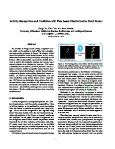
Figure 1. Three levels of representation in HAN for an example video.
There have been many approaches to the problem of activity recognition, many of which are hard to apply to the stated problem of fine-grained activity recognition. The human locomotion in this problem is of low inter-class variability so not very discriminative. Human pose is of obvious importance but the current pose estimation algorithms are not robust enough to provide discriminative pose configurations [23]. Hence, we resort to use of low-level features which has proved effective for many tasks. However, the distinctions between various activities in the finegrained task are small so similar activities may be difficult to discriminate. We propose that recognition of such activities can be significantly improved by grouping and decomposing them into a hierarchy of multiple abstraction layers. The recognition can then be guided by classifiers operating at multiple levels; furthermore, descriptions of varying abstractness are also generated which may be useful for different tasks. Use of such a hierarchy has been successfully explored for image classification [5] problems but not for activities, to the best of our knowledge. We describe an abstraction hierarchy model named Hierarchy Activity Network (HAN), which includes Meta level(s), Base level and Infra level(s), as shown in Figure 1. Base level is the level at which annotations are provided in the training data. Meta levels group some of the base level activities into one, resulting in more abstraction activities. Infra levels decompose a set of base level activities based on Infra distinctions. In the example, and in our experiments, we use only one meta and one Infra level but the technique
1. Introduction Activity recognition has been a popular topic of research in computer vision. The range of activities can vary broadly in terms of their specificity. In this paper, we focus on fine-grained activities that take place in a fixed environment, which has potential applications in intelligent home, elder people care and for daily living assistance. Several activities of daily life datasets have been introduced. A recent one is given in [23] which contains 65 different but similar kitchen activities. The characteristic that these activities take place in a fixed (and possibly known) environment can be helpful but also prevents environmental context from being a key distinguishing feature. Furthermore, the activities of interest can be very similar, e.g. recognizing cutting stripes vs cutting slices in kitchen tasks. Considerable progress has been made in classifying such videos, [23][24] but accuracy remains low for many of the activities. 1
easily extends to the multiple levels. Note that this hierarchy is based on abstraction levels rather than the more common hierarchy derived from temporal decompositions as in, for example, [22][28]. Construction of Meta and Infra levels from Base level is by unsupervised clustering based on similarity using SVM classifiers. As we lack annotations at the Meta and Infra levels, the nodes may not have semantic names. For the Meta levels, we can create a name by composition of terms in the Base level. For Infra levels, it is difficult to provide a semantic name in unsupervised way, but we can relate the activities to attributes to construct meaningful phrases. Independent classifiers are trained for each node in the hierarchy. We use the score of a path in the network to compute the confidence of labels for a video. We find that this not only improves recognition accuracy but also gives us a better attribute prediction and description for the video. With the annotated attributes provided by [24], each Infra level node is associated with an attribute distribution learned from the training data. To generate Infra level descriptions, we use pre-trained attribute detectors in the video level. Thus, the attribute prediction in HAN for video is not only based on the binary attribute classifiers, but also the Infra level node priors. In activity classification task, we do not use attribute annotations. We find that annotation for fine grained activity recognition has two limitations. First, the activity labels can be confusing; for example, it is hard to tell the difference between put in pan or pour in annotated video clips. Also, people have different opinions about when an activity starts, and when it ends. For example, it is hard to determine whether the activity open the fridge includes walking towards the fridge. We find that a better annotated video will help improve the classification performance. So we propose an automatic way to improve the annotation. We first prepare a video feature dictionary based on previous annotations. Then we evaluate the feature dictionary using trained model, replace the original feature with a candidate feature with highest confidence score, into a new training dataset. Then we iterate this process to get the final result. In summary, our contributions are: (1) Modeling of the mutual and hierarchy information within fine grained activities. (2) HAN’s hierarchy is of abstraction type which is different from and complementary to the more common temporal hierarchy (from atomic action to activity to events). (3) Demonstration that activity hierarchy helps improve fine grained activity recognition and attribute predictions. (4) A self updated annotation method improves both the classification performance and annotation quality. The paper is organized as follows. Section 2 discusses related work. Then, we introduce HAN in Section 3, including construction and inference using HAN. We present
experimental results in Section 4 and give our conclusions in Section 5.
2. Related Work A considerable number of approaches have been proposed in activity recognition problem. In complex datasets such as UCF101 [26] and HMDB51 [12], low and middle level features [29, 27, 11] are used commonly. Among them, the bag of spatial-temporal interest points [15] representation, patches [10], attributes [18], dynamic poselet[30], have been widely adopted for human action recognition. It can be combined with various models such as discriminative classifiers [16][21], unsupervised generative models [32], and semi-latent topic models [31]. Besides this holistic representation, researchers also work on integrating feature sequence arrangement and temporal ordering information. Some researchers try to construct plausible temporal structures [9] for different actions agents, but they ignore the temporal composition within the movements of a single subject under the framework of holistic representation. On the other side, temporal context based discriminative models can be applied in coarse grained activities’ classification tasks [4]. Besides, contextual information, such as background scene context [21] and object interactions [9][33], can also improve the performance of activity recognition. Our paper uses an abstraction hierarchy which incorporates contextual information in both the training and testing stages. Fine grained image or activity classification poses further challenges. One is that the training data is limited due to the difficulty of acquiring fine grained annotations. Besides, unlike categorization, the differences between fine grained classes may be subtle and only some key features may be useful. One approach to address these problems is to apply specialized domain knowledge [13], which uses botany information to help classify leaves. However, this requires developers to have a deep understanding of the specific field. Another method is to use crowdsourcing in the loop [7][3], asking humans to either label or propose parts and attributes [2][1], which achieves promising results. The difficulty lies in designing annotation tasks effectively: two ways are proposed to solve this problem. One is ask humans to label pre-defined parts and attributes [7][3], which requires careful design; the other is to use open-ended tasks [19]. But the quality in this method may be hard to control and descriptors may be highly varied. The recent improvement for ImageNet is [5], which introduces Hierarchy and Exclusion (HEX) graphs to captures semantic relations between any two labels applied to the same object: mutual exclusion, overlap and subsumption. Similarly, [8] propose a solution when we cannot find an accurate prediction for a pre-trained model, it finds a less specific answer that is also plausible from a pragmatic standpoint.
Figure 2. HAN Flow Chart and Representation. We first build Meta and Infra level in an unsupervised way, then integrate these nodes into an abstraction hierarchy model. HAN can be used to classify activities and predict attributes in a given input video.
Recently, [34] shows large improvements on the [23] fine grained activity dataset using pre-detection of objects. They take advantages that most of the objects are stationary, and the video is captured with a fixed camera (strong prior integrated). However, it is difficult to generalize this approach as reliable object detectors which are not always available. In our HAN solution, we never use the pre-detection objects, no extra annotations are needed. [25] discusses about how to find the most discriminative portion of videos, while we focus on auto improving the fine grained activity annotations and achieving better recognition performance.
3. Hierarchy Activity Network In this section, we give a description of how to model HAN and apply it for activity recognition. First, we define HAN model and activity similarity in detail. Next, we show how to encode the semantic similarity information to construct HAN model in an unsupervised way. In the third part, we show how to apply HAN in fine-grained activity recognition and use HAN to generate description in different hierarchy activity levels. The flow chart of HAN is shown in Figure 2.
3.1. HAN Representation HAN is a multiple level network which integrates information from not only the Base level, but also Meta (super) level and Infra (sub) level. The design of Meta level and Infra level follows two intuitions in the fine grained activity recognition problem. On one hand, some similar base level activities with limited training samples need a meta classifier to help distinguish from other uncorrelated activities. For example, Cut Something helps distinguish finer cutting activities (e.g. cut stripes) from other non-cut activities. On the other hand, for certain activity, there may still exist different sub-actions like take&put in fridge, spread. These sub-actions may be hard for one general classifier to recognize. Thus, we need to build Infra level to further select
discriminative sub clusters. Here we give the definition for these three levels specifically. Base Level: This is the level where the main video labels are provided and where the activity recognition tasks are defined. Meta Level: This is the more abstract level of the base level. It groups some of the activities in base level by combining similar base level activities. Infra Level: This is the more detailed level below the base level. Each activity can be divided into several Infra level nodes in an unsupervised way. If the dataset provides attribute annotations, each Infra node can own discriminative attributes distribution in this level. We denote Bi for the nodes in the Base level, Mj for each synthesized node in the Meta level, and Fk for the nodes in the Infra level. The confidence for Bi is denoted as f (Bi |φ(x)), where φ(x) denotes input feature for sample x. An example representation of HAN model is shown in Figure 2. Similarity Measure: HAN automatically generates the Meta and Infra levels. To build such a network, we need a similarity metrics. As no similarity annotation is provided, we choose to use one versus one SVM distance for the similarity measure. We define a similarity matrix S on the training dataset. Sij represents the similarity between Activities Bi and Bj . We use training samples from activity Bi and activity Bj in base level as an example. To get Sij , we train SVM using Bi as positive and Bj as negative. For each labeled Bi or Bj pair, we get a confidence score. We then compute the average for these two groups of samples. Last, we compute their difference from the average score. The distance between activity Bi and Bj is computed by the following formula. 1 X (f (Bi |φ(xk )) − f (Bj |φ(xk ))) (1) Sij = T k
where {xk } denotes the training samples with size T .
3.2. HAN Construction We first analyze the benefits of building meta level and Infra level using SVM classifier [20] as an example. Then we state the detailed method of constructing HAN model. Generating the Meta level: If we use hinge loss function for optimization, the primal form of objective function can be written as: 1 k w k22 (2) 2 n where C ≥ 0, {ξn } are slack variables, which also represent the hinge loss function: L(w) = C
X
ξn +
`(w) = max(0, 1 − y[w> φ(x) + b])
(3)
For misclassified samples, the hinge loss is proportional to the difference between estimation probability of true label class i and wrong estimated label class j: `(w, φ(xn )) ∝ f (Bj |φ(xn )) − f (Bi |φ(xn ))
(4)
Summing the hinge loss function for class i, we get: X X `(w)i = `(w, φ(xin )) ∝ − Sij
(5)
n
j
where {xin } denote the sample set with true label i. From Equation 5, we observe that L(w) in Equation 2 can be reduced by dropping the loss generated from the first t smallest elements in i th column of similarity matrix S. Thus, we can use S to merge different similar activities classes into one Meta level node Mk , which is the corresponding node in Meta level. In training stage for certain class Bi , we eliminate similar samples from different classes Bj sharing the same Mk . After we generate S using Equation 1, we apply a greedy method to select most similar pairs of activities, as shown in Algorithm 1 below. Algorithm 1 Similar Activity Pair Selection Input: similarity matrix S 1: Label all Bi “available” 2: while there is activity classes available do available 3: Find (i, j)∗ = arg mini,j Sij 4: Change activity Bi , Bj ’s labels as “unavailable” 5: Add (Bi , Bj ) to merge list L 6: end while 7: for k th pair in L do 8: Assign Mk two children node: Bi , Bj 9: Set path(Bi , Mk ) = 1, path(Bj , Mk ) = 1 10: end for 11: return Mk With SVM, similar examples are still hard to be separated, while the not similar examples are easy to be separated.
Figure 3. Meta Level Generation Examples.
It is intuitive that the similar categories will still have less difference than the not similar categories. Using the SVM metrics, we find that screw open & screw close, wash objects & wash hands, cut stripes & cut slices belong to the same meta level nodes. Both intuition and experimental results shows the SVM metrics is more reasonable than equalweight distance metrics. Naming the Meta Level Nodes: The semantic names for Mk are synthesized from the activity names Bi and Bj . Typically, the activity name of Bi is composed like Do Object (verb + noun) or Do (verb). For an input activity name, we first use WordNet to decide which is verb, and noun in the name of Bi automatically. Then, we generate Meta level names using a synthesis rule as (vi + ni ) + (vj + nj ) = p(vi , vj ) + p(ni , nj ). Here p(vi , vj ), p(ni , nj ) mean the least shared parent of the verb and noun. For p(ni , nj ), we use the WordNet Hierarchy provided by ImageNet [6]. For example, we need to find the least share parent for pan and bowl. A path goes up to top from pan is, pan - container instrumentality. The path goes up from bowl is bowl - dish container - instrumentality. Therefore, the least shared parent of pan and bowl is container. For the verb p(vi , vj ), we temporally use human to name their parent verb due to the challenges in building verbs mutual relations. In this way, we can synthesis the Meta level node names like put in pan + put in bowl = put in containers. Generating the Infra Level: The function of Infra level is to provide more detailed description for each activity class by clustering them, making a Infra sub class. To achieve this goal, we prepare two protocols to constrain the division of fine grained training samples: first, the samples need to be roughly equal distributed; second, the intraclass distance needs to be as small as possible. We use K −means clustering to select the most discriminative feature groups for representing different sub-activities. The two protocols are encoded in constraints of clusters’ sizes balancing and minimizing the total distance sum:
D(K, {xi }) =
K X k=1
! Nk 1 X ynk d(φ(xn ), Ck ) Nk n=1
(6)
where d(φ(xn ), Ck ) denotes the distance for each feature φ(xn ) to its center Ck . ynk = 1 if φ(xn ) belongs to kth cluster, otherwise ynk = 0. For building Infra level, we use a loop to find the best Infra level separation with K-means. Our algorithm balances
ω · ψ(p, x): p? = arg max ω · ψ(p, x)
(7)
p
Figure 4. Combining an Infra level Node with Attributes.
the training sample number for each sub class so that possible solutions for unsupervised classification will be limited.. Then, we use SVM to train the Infra level nodes according to the separated data. Naming the Infra Level Nodes: It is difficult to automatically give the Infra level nodes a semantic name (as the Infra level nodes are generated in an unsupervised way.) Therefore in Infra level, instead, we attach a template of semantic attributes for each input video, using predicted attributes as explained below. In the kitchen dataset, the attribute annotations are given [24] and can be used in training. Boosting Infra Level with Attributes: HAN can optional integrate activity attributes in a supervised way. This allows the infra nodes to contain attribute priors which can then be combined with attribute detectors for improved descriptions. We generate sentence descriptions by filling in predicted attributes into pre-defined sentence templates. Four attributes are provided: actions (e.g. take out), tools (e.g. hand, knife), ingredients (e.g. apple), and containers (e.g. baking tray, bowl). Given the attribute values, we can compose a sentence: for example, given Action = taking out, tool = hand, ingredient = bottle, containers = fridge, we can generate the sentence : Person takes out a bottle using hand (from the fridge). Summary: To give difference level descriptions, for the Meta level, we use the synthesis name of predicted node Mj . For the Base level, we use name of predicted base node Bi . For the Infra level, we use the predicted attributes to compose a sentence. We introduce how to predict the attributes in next section.
3.3. HAN Inference Activity Recognition: For each input video x, we calculate a coarse to fine path p in HAN. Every path is composed of a node from the Base level Bi , a node from the Meta level Mj , and a node from the Infra level Fk . It can be written as p = (Bi , Mj , Fk ). Given input video x, we define a vector ψ(p, x), which ψ(p, x) = [φ(Bi ), φ(Mj ), φ(Fk ), ϕ(Bi , Mj ), ϕ(Bi , Fk )]. The φ(Bi ), φ(Mj ), φ(Fk ) are the unary confidences of selecting Bi , Mj , Fk to represent the videos. Specifically, φ(Bi ) is the output of a single binary video classifier. ϕ(Bi , Mj ), ϕ(Bi , Fk ) are the pairwise term that shows how likely the path is. It is set equally in our implementation. The optimal path p∗ is given by maximizing the output of
where the ω is the weight for ψ(p, x), to balance each term. ω is set equally at the initialization, then we search these parameter and choose the weight by cross validation on training dataset. Attribute Prediction: Within the Infra level, activity attributes are predicted as follows. We first train the video level attribute detectors using middle level features and an SVM [20]. Assuming a base level node Bk is decomposed into Infra nodes Fki , we predict attributes for node Bk by the following formula: a? = arg max φ(ai )
X
ai
p(ai |Fkj )φ(Fkj )
(8)
where φ(ai ) is the confidence for the trained attribute detector, φ(Fkj ) is the confidence for the Infra node Fkj . p(ai |Fkj ) is the prior where p(ai |Fkj ) =
Nai ,Fkj NFkj
. Nai ,Fkj
is the number of samples that belong to node Fkj with the attribute ai , while NFkj is the total number of samples that belongs to node Fkj . Note that this combines the prior expectations of attributes for a specific node with the actual detector outputs.
3.4. Auto Annotation Updating The annotation for fine grained activity needs refinement. We propose an auto annotation updating method. For the training dataset T , we break them into N subset Ti . For each Ti , we leave most of the original training data (where Tj , j 6= i) in training data set T1 , and we use the Ti for improvement in set T2 . For each example in T2 , we prepare a feature expansion dictionary D, by re cropping the sample from T2 . For example, if we have a sample Xi from T2 , we generate the Xij by modifying the boundary of sample Xi , put all Xij into our dictionary. Then, we train a detector using the samples from T1 , and test them on T2 . We sort the results and find the best cropped video clips in D, then update the original Xi in T2 . Using a similar strategy, after we updates the whole training dataset, we train a new fine grained activity detector. The specific algorithm is shown in Algorithm 2.
3.5. Discussion on Hierarchy Building hierarchy has been used in image classification problem. [17] builds the tree from the top down: the leaf level is the recognition target. Our idea is to extend the target layer, by combining nodes into meta level, and decompose nodes into finer level. The semantic hierarchy idea is novel for the activity recognition problem. In activity recognition problem, [14] has a different hierarchy concept than our paper. They consider viewpoints
Algorithm 2 Auto Annotation Update SN Input: Feature dataset T = i=1 Ti , (Ti ∩Tj = ∅, i 6= j) 1: for each subset Ti do SN 2: Generate specific training set Ci = j=1,i6=j Tj 3: Generate feature dictionary Di = f (Ti ), where f (.) denotes the time-shift and time-truncation operations on the samples {xij } in Ti 4: Train activity detector Mi on Ci 5: for j = 1 to |Ti | do 6: Find expanded feature set dij = f (xij ) for xij 7: Apply detector Mi on dij to generate scores sij i 8: Select the optimal feature: xi∗ j = arg maxdij sj 9: Replace the original feature: xij ← xi∗ j 10: end for 11: end for 12: return T
and poses to create a hierarchy; in other words, an appearance hierarchy whereas ours is a semantic hierarchy. Also, our predicted multi-level description is not based on the basic-level category annotations, which is different from their method.
we use leave-one-person-out cross-validation but only for the 7 actors that are specified to be test subjects to be consistent with the experiments settings in [23]. For accuracy of classification, we use the same evaluation criteria and code provided by [23]. This consists of measuring average precision (AP) for each class and a mean average precision (mAP) across all the classes.
4.3. Meta and Infra Level Generation We use the unsupervised learned similarity measure to build the Meta level (described in Section 3.1). In this evaluation, we combine 64 Base level nodes (we neglect the background activity) into 32 Meta level nodes. Figure 3 shows part of HAN structure which demonstrates the similarity pairs explored, and the synthesized nodes by combining them into Meta level nodes. For the Infra level nodes, we use the K-means clustering to cluster nodes, as described in Section 3.2. We do not decompose Base level nodes that have much less than 10 samples. For others, we divide them into 2 to 4 Infra nodes each, depending on how many training samples each base node has; we maintain around or greater than 10 training samples per Infra node. In the kitchen dataset, we generate a total of 128 Infra nodes.
4. Experimental Results
4.4. Classifier Training
We test HAN on the most widely used fine grained activity dataset [23]. We first introduce the dataset specifications and experiment setup, and then provide the results.
We train classifiers for nodes at each level by using libsvm with Histogram Intersection Kernel (HIK) [20]. For the base level nodes, we use similarity pairs to help refine positive and negative training examples. If we are training the base level node for activity Bi (the most similar class is activity Bj ), we need to use examples with label Bi , and the negative examples should exclude label Bj ’s examples. Similarly, we do not use examples from sibling nodes for the Infra level nodes as well. Note that this distinction is made possible by the use of HAN structure.
4.1. Dataset This dataset contains 12 different actors, 44 videos, 5609 clips, 881755 frames. It contains 65 fine-grained activities (listed in a results table later, except one is background activity). It includes challenging tasks such as recognizing the difference between cut dice and cut slices, take out from drawer and open/close drawer. HAN focuses on fine-grained activity recognition which is not the same type dataset as Hollywood and HMDB. In non fine-grained activity recognition dataset, clustering high inter-class variance activities will help less.
4.2. Experiment Setup We use the middle video level features provided by [23]. These include Histogram of Oriented Gradients (HOG), Histogram of Oriented Flow (HOF) and Motion Boundary Histograms (MBH). The features were generated around densely sampled points, which are tracked for 15 frames in a dense optical flow field. For feature histograms, 4000 words, obtained by K-means clustering over a million sampled features, were used for each type of feature. We use the same train and test split as in [23]. We use one actor’s data as testing; the rest (11) for training. Thus,
4.5. Classification Results We compute scores for classifiers trained separately for HOG, HOF and MBH features. We combine the results of the three features by averaging their confidence values. Table 1 shows the mAP results for the three features and their combination for various configurations. The first two lines, showing the published baseline results and just the Base layer of HAN are almost the same. The next two lines show that each of the two levels improves accuracy over the baseline. The last line shows the results using the entire HAN structure. Note that using MBH features alone, HAN improves results by 8.5% compared to the baseline; combined improvement is 5.4% in mAP. The dataset also includes pose information but we did not experiment with this feature, as the baseline [23] shows these features to give a low mAP (34.6%)
Method change temperature cut off ends dry lid: remove open tin open/close oven pour put in pan/pot read screw close spice stir take & put in fridge take out from cupboard t. out from spice holder wash hands
[23] 73.6 16.3 97.4 14.5 79.5 100 70.7 24.6 55.4 50.3 47.3 77.7 56.9 90.8 87.4 56.1
HAN 75.2 21.1 96.2 11.1 88.5 100 70.5 35.0 53.2 48.8 46.9 74.4 60.5 93.1 75.4 51.6
Method cut apart cut out inside fill water from tap mix open/close cupboard package X pull out put on bread/dough remove from package screw open spread strew take & put in oven take out from drawer taste wash objects
[23] 38.4 46.8 67.2 37.6 80.4 47.6 61.9 51.5 42.8 58.7 10.0 43.5 100 93.8 42.4 80.6
HAN 39.4 52.1 100 73.5 79.9 65.5 100 48.8 38.2 58.3 38.0 61.6 100 93.3 41.0 79.1
Method cut dice cut slices grate move from X to Y open/close drawer peel puree put on cutting-board rip open shake squeeze take & put in cupboard t. & put in spice holder take out from fridge throw in garbage whisk
[23] 35.9 54.0 72.6 54.8 83.7 84.2 75.9 29.5 16.7 95.2 98.3 46.0 89.8 94.0 95.9 94.4
HAN 38.5 51.0 70.5 54.5 79.6 79.0 100 35.1 12.3 93.9 100 46.0 89.1 80.2 96.4 93.8
Method cut in cut stripes lid: put on open egg open/close fridge plug in/out put in bowl put on plate scratch off smell stamp take & put in drawer take ingredient apart take out from oven unroll dough wipe clean
[23] 21.9 34.4 20.1 67.4 96.8 61.9 34.5 26.9 6.4 87.4 64.6 43.2 42.1 100 45 12.8
HAN 21.9 56.2 6.5 63.6 95.5 69.8 37.7 25.9 28.7 87.4 100 53.9 50.7 100 100 41.6
Table 2. Average Precision for Individual Base Level Activities Recognition.
Method [23] Base Base+ Meta Base+ Infra HAN
HOG 52.9 48.7 54.1 53.5 53.9
HOF 53.4 49.2 53.4 54.3 54.9
MBH 52.0 54.4 58.8 59.7 60.5
Combine 59.2 59.1 62.5 63.5 64.6
Table 1. Mean Average Precision numbers for different features and network configurations. Note that complete HAN framework with combined features achieves the best result.
In recent work, [34] has reported mAP of 70% on the same dataset. However, they use knowledge of pre-detected objects, such as the cabinets and refrigerator; hence, we do not consider these numbers to be directly comparable. One can argue that such objects could be known in a fixed environment but, nonetheless, this reduces flexibility. Without the use of knowledge of fixed objects, accuracy of [34] is 59.2%, which is lower than our result using HAN. For the activity classification task, we do not use the attribute annotation provided by [23]. In Table 2, we show mAP performance for individual activity types. Within the 64 fine grained activities, HAN gives better results than [23] in 28 activities. Notice that improvements for several activities are quite large and in 5 classes, AP rises to 100%. Performance is improved for many challenging activities such as cut. The Meta level node Cut Something helps distinguish finer cutting activities (e.g. cut stripes) from other non-cut activities. Similar improvements are also observed for the base activities put in bowl and put in pan/pot. Infra level nodes can also help improve precision for decomposable activities. We can see that the take& put in drawer and take& put in fridge both benefit from decomposing the complex actions (take and put in.) Spread involves varying ingredients (bread, butter and oil), different tools (spoon, knife and hand) which cause high intra-class variance. Decomposing these types of base nodes into Infra nodes helps improve the video classification results.
Figure 5. Output of HAN on two test videos. Coarse to fine descriptions are shown.
To show the performance of HAN, we use the feature provide by our baseline paper. All the experiment settings are the same except we add in HAN hierarchy (We use the exactly same feature provided by [23]). Second, kitchen dataset is very challenging. Few paper use this dataset because the result in [23] is hard to exceed.
4.6. Infra Level Attribute Experiments In this section, we describe performance of attribute prediction in Infra Level. The Infra level description is composed by four attribute types: actions, tools, ingredients and containers. The attribute annotations are provided from [23] and used during training and for evaluation. Single attribute detectors are trained using a linear SVM and features provided from [23], which are applied in both Base and Infra level nodes. The train and test splits are the same as for video level classification. We use HAN to predict attributes as described in Section 3.2 for each category. Then we use them to fill in a sentence template to describe the activity; some of the outputs are shown in Figure 5. For quantitative evaluation of generated attributes, we calculate the mAP for each category. We find that among the 218 attributes provided from [23], several come with very few annotation examples; precision for these attributes is not reliable so we only include attributes that have at least 50 annotated samples. Under this criteria, there are 20 such attributes in the action category, 5 in the tool category, 7 in the container category, and 19 in the ingredients category. The baseline uses outputs of the attribute detectors only,
Method Attribute Att + HAN
Action 59.69 65.03
Container 47.38 49.95
Tool 71.48 72.36
Ingredient 29.97 32.41
Table 3. Attribute mAP evaluation.
Attribute Name add (Action) change temperature put in take apart baking tray (Container) bowl counter cutting board drawer pan pot apple (Ingredient) bottle carrot cheese onion orange paper box spice shaker
Attribute 42.72 51.22 59.05 27.41 21.82 30.03 30.64 81.78 64.85 66.61 35.91 28.42 56.25 9.60 6.67 13.43 23.14 17.57 73.26
Attribute + HAN 49.56 54.38 66.51 46.92 14.28 35.39 35.18 85.52 67.35 78.37 33.57 29.81 55.10 11.47 10.84 23.37 29.05 23.60 86.98
Table 4. Average Precision for part of Action Attributes, Container Attributes, and Ingredients attribute.
while our method integrates HAN into the prediction. The results are given in Table 3. HAN improves attribute prediction by 5.4% for action attributes, 2.6% for Container attributes, 1% for the tool category and 2.5% in ingredient category. In total, we improve for about 3% in average. In detail, we show the accuracy of attribute results for four actions in Table 4. We observe that HAN improvements are higher in actions that have high intra-class variability. In Base level, take ingredient apart is of high variance, because the ingredients can be tomato, orange, dough, the tools can be hand and knife; also each actor has different ways of performing this action. Decomposition of base level node helps increase accuracy by clustering similar examples. Take & put in activity is also high in intra-class variations as it involves different containers such as drawer, fridge and cupboard; again, decomposition shows high improvements. On the other hand, change temperature has few variations and decomposition does not improve accuracy by much. Table 4 shows attribute prediction results for containers. HAN improves results for 5 of the 7 container attributes. Table 4 shows attribute prediction results for ingredients. HAN improves results for 13 of the 19 ingredient attributes. The improvements come about, because HAN brings in ac-
Method HAN HAN + Expand=9 HAN + Expand=16
HOG 53.9 54.3 54.1
HOF 54.9 56.4 56.8
MBH 60.5 63.6 64.7
Combine 64.6 66.4 67.8
Table 5. Self Annotation Update Improvement
tivity/objects context: for example, cheese is often related to the strew activity, and orange is often related to the squeeze activity.
4.7. Annotation Update Experiment As we have 12 subjects, we use 10 subjects as a training set (T1 set), 1 subject for annotation improvement (T2 set), and 1 subject as test data. Using the method described in Section 3.4, the annotations are updated in T2 . Similarly, we update the annotations for videos in subset in T1 . After one round of iteration, we get improvement of 3.2%, achieving 67.8% mAP in total based on HAN. We compare to the original result in Table 5 with two experiment set expansion =16/interval =0.1, expansion =9/interval =0.1 (using the same feature provided in [23]). In detail, for each feature in T2 (when per feature expansion = 16, interval=0.1, total video length = t), we pick a start time point from candidate pool [0, 0.1t, 0.2t, 0.3t], and pick a end time point from candidate pool [0.7t, 0.8t, 0.9t, t]. In this way, one origin feature will expend to 16 features. Annotation Quality: In our experiment, we find that around 23.2% video clips need annotation boundary refinement. After sorting the results, we find that the annotation for Fridge / Drawer / Cupboard related activities are ambiguous. That might be because of the open fridge includes walking towards the fridge, Take out from fridge includes partial open/close fridge, Take out from drawer includes partial open/close drawer. Also, whether throw in garbage should include collect garbage before throwing. Annotation for fine grained activities is challenging, and auto annotation updates help improve classification performance.
5. Conclusion We described a new semantic hierarchy model for activity recognition named HAN. Unlike previous temporal level hierarchy models, HAN is based on an abstraction hierarchy. It includes three different levels which can describe the videos from coarse grained to fine grained. We demonstrate that the use of HAN improves the accuracy of activity recognition and also provides improved attributes for description. HAN can be easily extended to multiple levels of hierarchy. It would be also interesting to explore incorporating these levels into a temporal hierarchy for longer duration activities. Acknowledgment: This research was supported, in part, by the Office of Naval Research under grant N00014-13-10493.
References [1] L. Bourdev, S. Maji, T. Brox, and J. Malik. Detecting people using mutually consistent poselet activations. In Proc. ECCV, 2010. 2 [2] L. Bourdev and J. Malik. Poselets: Body part detectors trained using 3d human pose annotations. In Proc. ICCV, 2009. 2 [3] S. Branson, P. Perona, and S. Belongie. Strong supervision from weak annotation: Interactive training of deformable part models. In ICCV, 2011. 2 [4] S. C., Kanaujia, and A. Metaxas. Conditional models for contextual human motion recognition. In CVIU, 2006. 2 [5] J. Deng, N. Ding, Y. Jia, A. Frome, K. Murphy, S. Bengio, Y. Li, H. Neven, and H. Adam. Large-scale object classification using label relation graphs. In ECCV, 2014. 1, 2 [6] J. Deng, W. Dong, R. Socher, L.-J. Li, K. Li, and L. FeiFei. Imagenet: A large-scale hierarchical image database. In CVPR, 2012. 4 [7] R. Farrell, O. Oza, N. Zhang, V. Morariu, T. Darrell, and L. D. Birdlets. Birdlets: Subordinate categorization using volumetric primitives and pose-normalized appearance. In ICCV, 2011. 2 [8] S. Guadarrama, N. Krishnamoorthy, G. Malkarnenkar, S. Venugopalan, R. Mooney, T. Darrell, and K. Saenko. Youtube2text: Recognizing and describing arbitrary activities using semantic hierarchies and zero-shot recognition. In ICCV, 2013. 2 [9] J. S. Gupta A., Srinivasan P. and D. L.S. Understanding videos, constructing plots learning a visually grounded storyline model from annotated videos. In CVPR, 2009. 2 [10] A. Jain, A. Gupta, M. Rodriguez, and L. S. Davis. Representing videos using mid-level discriminative patches. In CVPR, 2013. 2 [11] V. Kantorov and I. Laptev. Efficient feature extraction, encoding and classification for action recognition. In CVPR, 2014. 2 [12] H. Kuehne, H. Jhuang, E. Garrote, T. Poggio, and T. Serre. HMDB: a large video database for human motion recognition. In Proceedings of the International Conference on Computer Vision (ICCV), 2011. 2 [13] N. Kumar, P. Belhumeur, A. Biswas, D. Jacobs, W. Kress, I. Lopez, and J. Soares. Leafsnap: A computer vision system for automatic plant species identification. In ECCV, 2012. 2 [14] T. Lan, T.-C. Chen, and S. Savarese. A hierarchical representation for future action prediction. In ECCV, 2014. 5 [15] I. Laptev. On space-time interest points. In IJCV, 2005. 2 [16] I. Laptev, M. Marszalek, C. Schmid, and B. Rozenfeld. Learning realistic human actions from movies. In CVPR, 2008. 2 [17] M. M. lek and C. Schmid. Constructing category hierarchies for visual recognition. In ECCV, 2008. 5 [18] J. Liu, B. Kuipers, and S. Savarese. Recognizing human actions by attributes. In Proc. CVPR, 2011. 2 [19] S. Maji. Discovering a lexicon of parts and attributes. In ECCV Workshop, 2012. 2 [20] S. Maji, A. C. Berg, and J. Malik. Classification using intersection kernel svms is efficient. In CVPR, 2008. 4, 5, 6
[21] L. I. Marszalek, M. and C. Schmid. Actions in context. In CVPR, 2009. 2 [22] H. Pirsiavash and D. Ramanan. Parsing videos of actions with segmental grammars. In CVPR, 2014. 2 [23] M. Rohrbach, S. Amin, M. Andriluka, and B. Schiele. A database for fine grained activity detection of cooking activities. In CVPR, 2012. 1, 3, 6, 7, 8 [24] M. Rohrbach, M. Regneri, M. Andriluka, S. Amin, M. Pinkal, and B. Schiele. Script data for attribute-based recognition of composite activities. In ECCV, 2012. 1, 2, 5 [25] S. Satkin and M. Hebert. Modeling the temporal extent of actions. In ECCV, 2010. 3 [26] K. Soomro, A. R. Zamir, and M. Shah. Ucf101: A dataset of 101 human action classes from videos in the wild. In CRCVTR-12-01, 2012. 2 [27] C. Sun and R. Nevatia. Large-scale web video event classification by use of fisher vectors. In WACV, 2013. 2 [28] C. Sun and R. Nevatia. Discover: Discovering important segments for classification of video events and recounting. In CVPR, 2014. 2 [29] H. Wang, A. Klaser, C. Schmid, and C.-L. Liu. Action recognition by dense trajectories. In CVPR, 2011. 2 [30] L. Wang, Y. Qiao, and X. Tang. Video action detection with relational dynamic-poselets. In ECCV, 2014. 2 [31] Y. Wang and G. Mori. Human action recognition by semilatent topic models. In TPAMI, 2009. 2 [32] K. T. Wong, S.F. and R. Cipolla. Learning motion categories using both semantic and structural information. In CVPR, 2007. 2 [33] B. Yao and L. Fei-Fei. Modeling mutual context of object and human pose in human-object interaction activities. In CVPR, 2010. 2 [34] Y. Zhou, B. Ni, S. Yan, P. Moulin, and Q. Tian. Pipelining localized semantic features for fine-grained action recognition. In ECCV, 2014. 3, 7