Abstraction of Arrays Based on Non Contiguous Partitions - DI ENS
Recommend Documents
Abstract. Array partitioning analyses split arrays into contiguous parti- .... An abstract domain that partitions array elements according to semantic prop- erties .... version of cleanup, which is chosen to highlight the analysis difficulties. .....
Jan 27, 2011 - Michael A. Bender1, Sándor P. Fekete2, Tom Kamphans2â, and Nils Schweer2. 1 Department of Computer Science State University of New ...
Aug 8, 2013 - During most of the twentieth century experimental and theoretical biologists lived separate lives. As the authors of this book express it, âthere ...
Mar 24, 2015 - Keywords Parallel tasks · Contiguous scheduling · ... We will call such a situation a c/nc-difference. An ... For conciseness, we will be calling pj ...... partially supported by a grant of Polish National Science Center, a grant.
signatures of known messages can recover the secret signature key using a single computer in ... negligible probability of success to forge a valid signature, it can be transformed ..... Design, Codes and Cryptography, 23:283â290, 2001. 6.
May 23, 2012 - Abstract Authenticated Key Exchange protocols enable several parties to establish a shared ..... Besides the Secure Remote Password.
vice, the secret exponent is used to transform an input related to the message into a digital signature via modular exponentiation. Timings and power attacks, first ...
partial ordering C, least upper bound U, greatest lower bound N. The infimum L of L is NL, the supremum T of L is UL. (Birkhoff's standard reference book [2] ...
Jan 27, 2015 - (will be inserted by the editor). Mathematical modeling of lymphocytes selection in the germinal center. Vuk Milisic · Gilles Wainrib. January 27 ...
The Economics of Internet Search ... Search engines are one of the most widely used Internet .... Yahoo turned them down
tion of those program proof methods in the class of Floyd [7] invariant asser- tions method for proving total correctness of sequential programs. We introduce.
Jul 1, 2018 - and it is given as a continuous interval, in principle â no jumps, no holes). âNaturalityâ ... (Lesne, 2007) for a comparative insight into the mathe- ..... bypass the physico-chemical causal structure - or even ...... sense. Our
combine randomizable encryption and signatures to a new primitive as follows: ...... add a new member B without learning his certificate provided by the authority .... A digital signature scheme secure against adaptive chosen-message attacks.
encryption; but he cannot make a signature on an encryption of a new ...... A digital signature scheme secure against adaptive chosen-message attacks.
combine randomizable encryption and signatures to a new primitive as ...... A digital signature scheme secure against adaptive chosen-message attacks.
In particular we outline some weaknesses in the designs of ... cycles of one block encryption with a 128-bit key timing of the key setup is not included . Timing for ...
i.e. programs in which variables and array elements range over a numeric ... ables and a small number of iterations of the abstraction refinement loop usually ... We have implemented our procedure in the eureka tool and carried out sev- .... In the f
Markov chains, perfect simulation, queuing networks. 1. INTRODUCTION ..... n = 1; M := T; m := B; .... coupling time of PSA have the same distribution: Ïe =d Ï.
Antwerpen in 1989 [6] â appeared to have some weaknesses. The concept of designated ...... Advances in Cryptology - Crypto 2004 (M. K. Franklin, ed.), Lect.
... Ju Kim1, Seung Hwan Yoon2, Kyu Jung Cho3, Eugene Kim1, Young-Hye Kang1, .... Bone Impaction in Subaxial Cervical Spine Injury Jun Gu Han, et al.
Staphylococcus capitis is a coagulase-negative staphylococci (CoNS) commonly found in the human microflora. Recently, a clonal population of Staphylococcus capitis (denominated. NRCS-A) was found ..... ture contamination. Clin Microbiol ...
of automatic proofs and of symbolic calculi, it can also be stated that the basic ideas for the .... a lambda-term or for a functional program to have numerous types or to ..... to make room for this aspect, apparently not important for the mechanic
provider or to an email server, using a plaintext message. We define a new cryptographic primitive called plaintext-checkable encryption (PCE), which extends ...
Tufts University School of Medicine, Boston ... with C. Sonnenschein and A.M. Soto, biologists at Tufts University. ...... facing biological theorization â well beyond the computational parody. .... What genomes tell us, Harvard University Press.
Abstraction of Arrays Based on Non Contiguous Partitions - DI ENS
tition based techniques are unlikely to infer relevant partitions / precise array ... tricky invariants in an excerpt of the Minix 1.1 Memory Management Process.
Abstraction of Arrays Based on Non Contiguous Partitions ⋆ Jiangchao Liu and Xavier Rival INRIA, ENS, CNRS, Paris, France, [email protected], [email protected]
Abstract. Array partitioning analyses split arrays into contiguous partitions to infer properties of cell sets. Such analyses cannot group together non contiguous cells, even when they have similar properties. In this paper, we propose an abstract domain which utilizes semantic properties to split array cells into groups. Cells with similar properties will be packed into groups and abstracted together. Additionally, groups are not necessarily contiguous. This abstract domain allows to infer complex array invariants in a fully automatic way. Experiments on examples from the Minix 1.1 memory management demonstrate its effectiveness.
1
Introduction
Arrays are ubiquitous, yet their mis-use often causes software defects. Therefore, a large number of works address the automatic verification of array manipulating programs. In particular, partitioning abstractions [5,11,13] split arrays in sets of contiguous groups of cells, in order to, hopefully, infer they enjoy similar properties. A traditional example is that of an initialization loop, with the usual invariant that splits the array in an initialized zone and an uninitialized region. However, when cells that have similar properties are not contiguous, these approaches cannot infer adequate array partitions. This happens for unsorted arrays of structures, when there is no relation between indexes and cell fields. Then, there are usually relations among cell fields. This phenomenon can be observed in low-level software, such as operating system services and critical embedded systems drivers, which rely on static array zones instead of dynamically allocated blocks [20]. When cells with similar properties are not contiguous, traditional partition based techniques are unlikely to infer relevant partitions / precise array invariants. Figure 1 illustrates the Minix 1.1 Memory Management Process Table (MMPT) main structure. The array of structures mproc defined in Figure 1(a) stores the process descriptors. Each descriptor comprises a field mparent that stores the index of the parent process in mproc, and a field mpflag that stores the process status. Figure 1(c) depicts the concrete values stored in mproc to describe the process topology shown in Figure 1(b) (we show only 8 processes). An element ⋆
The research leading to these results has received funding from the European Research Council under the FP7 grant agreement 278673, Project MemCAD, and from the ARTEMIS Joint Undertaking no 269335 (see Article II.9 of the JU Grant Agreement).
2
Jiangchao Liu and Xavier Rival 1 struct mproc { 2 unsigned mpflag; 3 int mparent; 4. } mproc[24]; (a) Definition of array mproc
[0] : [1] :
fs
[2] :
init
1
fs 6
1 ≤ mpflag mparent = 0
usr1
1 ≤ mpflag mparent = 2
[4] :
free slot mm
1 ≤ mpflag mparent = 0
user process descriptor
0
1 ≤ mpflag mparent = 0
[3] :
system process descriptor
mm
usr0
1 ≤ mpflag mparent = 2
[5] : free slot
2
init
4
usr0
3
usr1
usr2
5
free
7
(b) Topology of processes
[6] :
usr2
mpflag = 0 1 ≤ mpflag mparent = 4
free
[7] : free slot
mpflag = 0
(c) A segment of mproc
Fig. 1. Minix 1.1 Memory Management Process Table (MMPT) structure
of mproc is a process descriptor when its field mpflag is strictly positive and a free slot if it is null. Minix 1.1 uses the three initial elements of mproc to store the descriptor of the memory management service, the file system service and the init process. Descriptors of other processes appear in a random order. In the example of Figure 1, init has two children whose descriptors are in mproc[3] and mproc[4]; similarly, the process corresponding to mproc[4] has a single child the descriptor of which is in mproc[6]. Moreover, Minix assumes a parent-child relation between mm and fs, as mm has index 0 and the parent field of fs stores 0. To abstract the process table state, valid process descriptors and free slots should be partitioned into different groups. Traditional, contiguous partitioning cannot achieve this for two reasons: (1) the order of process descriptors in mproc cannot be predicted, hence is random in practice, and (2) there is no simple description of the boundaries between these regions (or even their sizes) in the program state. The symbolic abstract domain by Dillig, Dillig and Aiken [8] also fails here as it cannot attach arbitrary abstract properties to summarized cells. In this paper, we set up an abstract domain to partition the array into non contiguous groups for process descriptors and free slot so as to infer this partitioning and precise invariants (Section 2) automatically. Our contributions are: 1. An abstract domain that partitions array elements according to semantic properties, and can represent non contiguous partitions (Section 3). 2. Static analysis algorithms for the computation of abstract post-conditions (Sections 4 and Section 5), widening and inclusion check (Section 6). 3. The implementation and the evaluation of the analysis on the inference of tricky invariants in an excerpt of the Minix 1.1 Memory Management Process Table (MMPT) and other challenging array examples (Section 7).
Abstraction of Arrays Based on Non Contiguous Partitions
Fig. 2. A partitioning of mproc based on non contiguous groups
2
Overview
The Minix MMPT requires mproc to permanently satisfy two invariants: 1. Each valid process descriptor has a mparent field, that should store a value in [0, 23], hence represents a valid index in mproc: this entails the absence of out-of-bound accesses in process table management functions. 2. The mparent field of any valid process descriptor should be the index of a valid process descriptor: as a process can only complete its exit phase when its parent calls wait, failure to maintain a parent for each process could cause a terminating process to become dangling and never be eliminated. To verify these invariants, we propose to check that all system calls preserve them. We design an automatic analysis to verify that, if they are called in a state that satisfies these invariants, they return in a state that also satisfies them. A concrete state is displayed in Figure 2(a), and its abstraction is shown in Figure 2(b). Group 0 contains only the process descriptor of init. Group 1 collects all free slots. Group 2 consists of all the valid process descriptors except that of init. The reason why we split init out into a separate group is that it is often treated in a special manner by OS routines. We let Gi denote the set of indexes of all the elements in group i. The abstract state shown in Figure 2(b) ties each group to properties of its elements. These will be formally defined in Section 3. By the Minix specification, the elements of group 2 satisfy the following correctness conditions C: – their indexes are in [0, 23], which we note 0 ≤ Idx2 ≤ 23 in Figure 2(b); – their flags are in [1, 63] (valid process descriptors have a strictly positive flag), \ 2 ≤ 63; which we note 1 ≤ mpflag \ 2 ≤ 23; – their parents are valid indexes, which we note 0 ≤ mparent – their parents are indexes of valid process descriptors, hence are also in group \ 2 ⊳ G0 ∪ G2 ; 0 or group 2, which we note mparent – the size of group 2 is between 0 and 23, which we note 0 ≤ Sz2 ≤ 23. Our abstraction relies on disjoint groups as other array partitioning abstractions [11,13]. However, our abstraction does not assume each group consists of a contiguous set of cells. The non-contiguousness of groups is represented by winding separation lines in Figure 2(b). To characterize groups, our abstraction relies
4
Jiangchao Liu and Xavier Rival
0 1 2 3 4 5
6
void cleanup(int child){ ... int parent = mproc[child].mparent; if (parent == 2){ mproc[parent].mpflag = 1; mproc[child].mpflag = 0; for(i = 0; i < 24; i++){ if (mproc[i].mpflag > 0) if (i! = parent) if (mproc[i].mparent == child) mproc[i].mparent = 2; } }else{. . .} . . .}
0
mm
1
fs
6
usr2
2
init
4
usr0
3
usr1
5
free
7
free
(b) Effect of cleanup
(a) A simplified excerpt of cleanup
Fig. 3. Minix 1.1 process table management, system function cleanup
not only on constraints on indexes, but also on semantic properties of the cell contents: while groups 1 and 2 correspond to a similar range, the mpflag values of their elements are different (0 in group 1 and any value in [1, 63] in group 2). Therefore our abstraction can express both contiguous and non contiguous partitions. In this example, we believe the abstract state of Figure 2(b) is close to the programmer’s intent, where the array is a collection of unsorted elements. We now consider the verification of Minix MMPT management procedures. We focus on cleanup, which turns elements of mproc that describe hanging processes into free slots. Figure 3(a) displays an excerpt of a simplified, recursion free version of cleanup, which is chosen to highlight the analysis difficulties. The call cleanup(4) in the state of Figure 2(a) will remove process usr0 and falls in that case; the result is shown in Figure 3(b): process usr2 becomes a child of init, while the record formerly associated to usr0 turns into a free slot. Function cleanup should be called in a correct Minix process table state and be applied to a child process in group 2, which we note child⊳ G2 . Figure 4 overviews the steps of the automatic static analysis of the excerpt of cleanup. The analysis proceeds by computing abstract post-conditions and loop invariants [3]. In this section, we focus on (1) cell materialization, (2) termination of the loop analysis and (3) removal of unnecessary groups. From the precondition, fields mparent of all elements in group 2 are indexes in groups G0 or G2 (abstract state at point 0 ). The test entails mparent is 2 at point 2 (corresponding to process init). Combining this, with the fact that group 0 has exactly one element (Sz0 = 1) at index 2 (Idx0 = 2), the analysis infers that parent can only be in group 0 (point 2 ). Therefore, the update at point 2 affects a group with a single element, hence, is a strong update, and produces predicate at point 3 . However, at that point, the next update is not strong, since mproc[child] may be any element of group 2, which may have more than one element (it has at least one element since child ⊳ G2 , thus Sz2 ≥ 1). Therefore, our domain materializes the array element being assigned by splitting group 2 into two groups, labeled 2 and 3. Both groups inherit predicates from former group 2. Additionally,
Abstraction of Arrays Based on Non Contiguous Partitions At point At point At point At point At point
group 3 has a single element (Sz3 = 1), thus the analysis performs a strong update and generates the abstract state of 4 . The analysis of all the statements in the program follows similar principles. We only discuss the termination of the analysis here, as our abstract domain has infinite chains (the number of groups is not bounded), hence the analysis of loops requires a terminating binary widening operator [3]. Widening associates groups of its inputs with groups of its result (ensuring the number of groups can only decrease to guarantee termination), and over-approximates group properties. After two widening iterations, our analysis produces abstract post-fixpoint 5 , where group 1 describes free slots, group 0 describes init, group 3 consists of child (just cleaned up) and groups 2 (resp., 4) represent valid process descriptors with indexes greater (resp., lower) than i. Our analysis can also decrease the number of groups, when some become redundant, e.g., when the analysis proves a group empty. For instance, the loop fixpoint 5 shows that indexes of elements in group 2 are greater than i. Thus, after the loop exit, any element of group 2 should have an index greater than 24, which implies this group is empty. Hence, this group is removed, and the analysis produces post-condition 6 , which entails correctness condition C (note that group 3, corresponding to child now describes a free slot).
6
3
Jiangchao Liu and Xavier Rival
Abstract domain and abstraction relation
In this section, we formalize abstract elements and their concretization. We describe the abstraction of the contents of arrays, using numeric constraints, in Section 3.1. Then, we extend it with relations between groups in Section 3.2. 3.1
The non-contiguous array partition domain
Concrete States. Our domain abstracts arrays of complex data structures. To highlight its core principle and simplify the formalization, we make two assumptions on the programs to analyze. First, there is no array access through pointer dereference (handling them would only require a product with a pointer domain), thus all array index expressions are of the form a[ex]. Secondly, all variables are either base type (e.g., scalar) variables (denoted by X) or arrays of structures (denoted by A). Structures are considered arrays of length 1, and arrays of scalars are considered arrays of structures made of a single field. A concrete state σ is a partial function mapping basic cells (base variables and fields of array elements) into values (which are denoted by V). We let N denote non-negative integers and F denote the set of fields. Thus, the set S of concrete states is defined by S = (A × N × F ∪ X) → V. More specifically, the set of all fields of elements of array a are denoted by Fa , and the set of valid indexes in a is denoted by Na . Non-contiguous array partition. Our analysis partitions each array into one or several groups of cells. A group is represented by an abstraction Gi of the set of indexes of its elements, where subscript i identifies the group. We let G denote the set of group names {Gi | i ≥ 0}. An array partition is a function p : A → P(G) which maps each array variable to a set of groups. We always enforce the constraint that groups of distinct arrays should have distinct names, to avoid confusion (∀a1 , a2 ∈ A, a1 6= a2 ⇒ p(a1 ) ∩ p(a2 ) = ∅). To express properties of group contents, sizes, and indexes, we adjoin numeric abstract values to partition p. This numeric information is split into a conjunction made of two parts. First, a global component ng constrains base type variables, group sizes and group fields. Group fields are marked as summary dimensions [10] in ng , that is as numeric abstract domain dimensions that account for one or more concrete cell(s), whereas base type variables and group sizes are non-summary dimension, i.e., each of them represents exactly one concrete cell. Second, for each group Gi , the index Idxi is constrained by a numeric abstract value ni . This second component is needed because our abstract domain allows empty groups, and when group Gi is empty, Idxi has no value, which is expressed by ni = ⊥. Intuitively, in the concrete level, Idxi denotes a possibly empty set of values (an empty group example will be provided in Section 7.2). − → To sum up, an abstract element is a pair (p, → n ) where − n is a tuple (ng , n0 , . . . , k−1 n ), and p defines k array partitions. Our abstract domain is parameterized by the choice of a numeric abstract domain N♯ , so as to tune the analysis precision and cost. In this paper, we use the octagon abstract domain [18].
Abstraction of Arrays Based on Non Contiguous Partitions a[0] a[1] a[2] a[3] a[4] a[5] a[6]
value = 2 value = −110 value = 2 value = −120 value = 8 value = −100 value = −100
7
p(a) = {G0 , G1 } G0
G1
0 ≤ Idx0 ≤ 4
1 ≤ Idx1 ≤ 6
\ 0 ≤ 8 ∧ −120 ≤ value \ 1 ≤ −100 2 ≤ value
ng : ∧
(a) Concrete array X
Sz0 = 3
∧
Sz1 = 4
(b) Abstract state a♯
Fig. 5. An abstraction in our domain
Example 1. Figure 5(a) displays a concrete state, with an array of integers a of length 7 (each cell is viewed as a structure with a single field value). Figure 5(b) → shows an abstraction a♯ = (p, − n ) into two groups G0 , G1 , where G0 (resp., G1 ) contains all cells storing a positive (resp., negative) values. This abstraction reveals the array stores no value in [−99, 1]. Concretization. A concrete numeric mapping is a function ν, mapping each base type variable to one value, each structure field to a non empty set of values and each index to a possibly empty set of values. We write γN♯ for the concretiza→ tion of numeric elements, which maps a set of numeric constraints − n into a set i of functions ν as defined above. The concretization γN♯ (n ) of constraints over group Gi is such that, when ni = ⊥ and ν ∈ γN♯ (ni ), then ν(Idxi ) = ∅. Then, γN♯ (ng , n0 , . . . , nk−1 ) = γN♯ (ng )∩γN♯ (n0 ) . . . γN♯ (nk−1 ). A valuation is a function ψ ∈ Ψ = G → P(Z), and interprets each group by the set of indexes it represents in a given concrete state. Additionally, we use the following four predicates to break up the definition of concretization: S def. Pv (ψ) ⇐⇒ ∀a ∈ A, Gi ∈p(a) ψ(Gi ) = Na ∧ (∀Gi , Gj ∈ p(a), i 6= j ⇒ ψ(Gi ) ∩ ψ(Gj ) = ∅) def.
Pb (σ, ν) ⇐⇒ ∀v ∈ X, ν(v) = σ(v) def.
Pi (ν, ψ) ⇐⇒ ∀a ∈ A, Gi ∈ p(a), ψ(Gi ) = ν(Idxi ) ∧ |ψ(Gi )| = ν(Szi ) def. Pc (σ, ψ, ν) ⇐⇒ ∀a ∈ A, f ∈ Fa , Gi ∈ p(a), j ∈ ψ(Gi ), σ(a, j, f) ∈ ν(b fi ) Predicate Pv (ψ) states that each array element belongs to exactly one group (equivalently, groups form a partition of the array indexes). Predicate Pb (σ, ν) expresses that ν and σ consistently abstract base type variables. Predicate Pi (ν, ψ) expresses that ν and ψ consistently abstract group indexes. Last, predicate Pc (σ, ψ, ν) states σ and ν define compatible abstractions of groups contents. Definition 1 (Concretization). Concretization γP is defined by: def. → → γP (p, − n ) ::= {(σ, ψ, ν) | ν ∈ γN♯ (− n ) ∧ Pv (ψ) ∧ Pb (σ, ν) ∧ Pi (ν, ψ) ∧ Pc (σ, ψ, ν)}
8
Jiangchao Liu and Xavier Rival
3.2
Relation predicates
The abstraction we have defined so far can describe non-contiguous groups of cells, yet lacks important predicates, that are necessary for the analysis. Let us consider assignment parent = mproc[child].mparent in cleanup (Figure 3(a)). Numeric constraints localize child in [0, 23], but this information does not determine precisely which group does cell mproc[child] belong to. In particular, the analysis will ignore from that point whether parent is the index of a valid process descriptor or not. To avoid this imprecision, we extend abstract states with relation predicates, that express properties such as the membership of the value of a variable in a group. They are defined by the grammar below: Definition 2 (Relation predicates). r ::= r ∧ r | true | v ⊳ Ga | b fi ⊳ Ga a G ::= Ga ∪ Gi | Gi
where v ∈ X where f ∈ Fa , Gi ∈ p(a) where Gi ∈ p(a) where Gi ∈ p(a)
a conjunction of predicates empty var-index predicate content-index predicate a disjunction of groups in a
A relation predicate r is a conjunction of atomic predicates. Predicate v⊳Ga means the value of variable v is an index in Ga , where Ga is a disjunction of a set of groups of array a. Similarly, predicate b fi ⊳ Ga means that all fields f of cells in group i are a indexes of elements of G . As an example, if Ga = G1 ∪ G3 , then v ⊳ Ga expresses that the value of v is either the index of a cell in G1 or the index of a cell in G3 . Example 2. We consider function cleanup of Figure 3(a). The pre-condition for the analysis of Figure 4 is based on correctness property C, hence partitions mproc in three groups, thus p(mproc) = {G0 , G1 , G2 }. Additionally, cleanup should be called on a valid process descriptor different from that of init, hence child should be in group G2 , which corresponds to predicate child ⊳ G2 . Then parent is initial\ 2 ⊳ G0 ∪ G2 , parent is a valid process ized as the parent of child. Since mparent descriptor index, and the analysis derives parent ⊳ G0 ∪ G2 . Hence, at point 1 , the analysis will derive relations r = child ⊳ G2 ∧ parent ⊳ G0 ∪ G2 ∧ . . .. Similarly, in the else branch of condition if (parent == 2), the analysis derives that parent ⊳ G2 . Concretization. We now extend the concretization to account for relations. First, we let ψ be defined on disjunction of groups, and let ψ(G0 ∪ . . . ∪ Gi ) = ψ(G0 ) ∪ → . . . ∪ ψ(Gi ). We write D♯ for the set of triples (p, − n , r). Definition 3 (Abstract states and their concretization). An abstract state → a♯ is a triple (p, − n , r) ∈ D♯ . The concretization γD♯ is defined by: → → γD♯ (p, − n , r) ::= {σ | ∃ψ, ν, (σ, ψ, ν) ∈ γaux (p, − n , r)} → − → − γaux (p, n , true) ::= γP (p, n ) → → γaux (p, − n , v ⊳ Ga ) ::= {(σ, ψ, ν) ∈ γP (p, − n ) | σ(v) ∈ ψ(Ga )} → − → − a γaux (p, n , fi ⊳ G ) ::= {(σ, ψ, ν) ∈ γP (p, n ) | ∀k ∈ ψ(Gi ), σ(a, k, f) ∈ ψ(Ga )} → → → γ (p, − n , r ∧ r ) ::= γ (p, − n , r ) ∩ γ (p, − n,r ) aux
0
1
aux
0
aux
1
Abstraction of Arrays Based on Non Contiguous Partitions G0
G0
G1
G0
G1
0 ≤ Idx0 ≤ 99
0 ≤ Idx0 ≤ 99
0 ≤ Idx1 ≤ 99
0 ≤ Idx0 ≤ 99
0 ≤ Idx1 ≤ 99
\0 = 0 value ∧ Sz0 = 100 r: i ⊳ G0
ng :
ng :
(a) a♯
\ 0 = 0 ∧ value \1 = 0 value ∧ Sz0 = 99 ∧ Sz1 = 1 r: i ⊳ G1
(b) split(a♯ , i)
9
\ 0 = 0 ∧ value \1 = 1 value ∧ Sz0 = 100 ∧ Sz1 = 0 r: i ⊳ G0
ng :
(c) create(a♯ )
Fig. 6. Partition splitting and creation in array a from abstract state a♯
4
Basic operators on partitions
In this section, we define basic operations on partitions (such as creation and merge), that abstract transfer functions and operators rely on. Splitting and creation. Unless specified otherwise, our analysis initially partitions each array into a single group, with no contents constraint. Additional groups get introduced during the analysis, by two basic operations: 1. Operator split replaces a group with two groups, that inherit the properties of the group they replace (also, membership in the old group turns into membership in the join of the new groups). It is typically applied to materialize a cell of a given index (in the group bounds) and enable a strong update. 2. Operator create introduces an empty group and is used to generalize abstract states in join and widening (note any field property is satisfied by the empty group; the analysis selects properties depending on the context). Both operators preserve concretization. → Example 3. Figure 6(a) defines an abstract state (p, − n , r) with a single array, fully initialized to 0, and represented by a single group. Applying operator split to that abstract state and to index i produces the abstract state of Figure 6(b), where G1 \ as is a group with exactly one element, with the same constraints Idx and value in the previous state. Similarly, Figure 6(c) shows a possible result for create. Merging groups. Fine partitions with many groups can provide great precision but may incur increased analysis cost. Therefore, the analysis can also force the fusion of several groups into one by calling operation merge on a set of groups. This is performed either as part of join and widening or when transfer functions detect some groups get assigned similar values. Example 4. Figure 7(a) defines an abstract state a♯ which describes an array with two groups. Applying merge to a♯ and set {0, 1} produces the state shown in Figure 7(b), with a single group and coarser predicates, obtained by joining the constraints over the contents of the initial groups.
10
Jiangchao Liu and Xavier Rival G0
G1
G0
0 ≤ Idx0 ≤ 99
0 ≤ Idx1 ≤ 99
0 ≤ Idx0 ≤ 99
ng : ∧ r:
\ 0 ≤ 5 ∧ value \1 = 1 3 ≤ value ∧ Sz1 = 50 Sz0 = 50 i ⊳ G0 ∪ G1
(a) a
♯
ng : ∧ r:
\0 ≤ 5 1 ≤ value Sz0 = 100 i ⊳ G0
(b) merge(a♯ , {0, 1})
Fig. 7. Merging in abstract state a♯
Reduction. Our abstract domain can be viewed as a product abstraction and can → → benefit from reduction [4]. In a♯ = (p, − n , r), components − n and r may help refining each other. For instance, in Figure 4, the analysis infers at point 1 that parent ⊳ G0 ∪ G2 and Idx0 = 2. Combining this with the numerical information derived from test parent == 2, the analysis should derive that parent ⊳ G0 (i.e., → parent is the index of init). Conversely, r may refine the information on − n : if child ⊳ G2 , then group G2 has at least one element, thus Sz2 ≥ 1. Such steps are performed by a partial reduction operator reduce, which strengthens the numeric and relation predicates, without changing the global concretization [4] (the optimal reduction would be overly costly to compute). This reduction is done lazily: for instance, the analysis will attempt to generate relations between i and Idxi only when i is used as an index to access the array Gi corresponds to. Basic operations split, create, merge and reduce are sound: Theorem 1 (Soundness). If a♯ is an abstract state, t an array, Gi a group, then γD♯ (a♯ ) ⊆ γD♯ (split(a♯ , t, Gi )) and γD♯ (create(a♯ , t)) = γD♯ (a♯ ). Moreover, if S is a set of groups, γD♯ (a♯ ) ⊆ γD♯ (merge(a♯ , t, S)). Similarly, reduce does not change concretization.
5
Transfer functions
Our analysis of C programs proceeds by forward abstract interpretation [3]. In this section, we study the abstract transfer functions for tests and assignments. 5.1
Analysis of conditions
In the concrete level, if ex is an expression, test ex? filters out states that do not let ex evaluate into TRUE. Its concrete semantics can thus be defined as a function over sets of states, by ∀S ⊆ S, Jex?K(S) = {σ ∈ S | JexK(σ) = TRUE}. Intuitively, the abstract interpretation of a test from abstract state a♯ = → − → (p, n , r) can directly improve the constraints in the numeric component − n , which can then be propagated into r by reduce. The numeric test will derive new constraints only over non summary dimensions, thus tests over fields of groups that contain more than one element will not refine abstract values.
Abstraction of Arrays Based on Non Contiguous Partitions
11
When a test involves an array cell as in a[i] == 0?, and if the group that cell belongs to cannot be known precisely, a more precise post-condition can be derived by performing a locally disjunctive analysis, that applies numeric test to each possible group, and then joins the abstract states. For instance, if i ⊳ G0 ∪ G1 , the analysis will analyze test a[i] == 0? for both i ⊳ G0 and i ⊳ G1 , join the results of both tests, and apply operator reduce afterwards. Note that the abstract test operator does not change the partition, thus this join boils down to applying the abstract join joinN♯ of numeric abstract domain N♯ and set intersection to relations viewed as sets of atomic relations. The resulting join operator, limited to cases where both arguments have the same partitioning is de→ → → − fined by join≡ ((p, − n 0 , r0 ), (p, − n 1 , r1 )) = (p, joinN♯ (− n 0, → n 1 ), r0 ∩ r1 ). It is sound: → − → − → − ∀i ∈ {0, 1}, γD♯ (p, n i , ri ) ⊆ γD♯ (join≡ ((p, n 0 , r0 ), (p, n 1 , r1 ))). Abstract transfer function test is sound in the sense that: ∀σ ∈ γD♯ (a♯ ), JexK = TRUE =⇒ σ ∈ γD♯ (test(ex, a♯ )) Example 5. We consider the analysis of the code studied in Section 2. At the beginning of the first iteration of the loop, i is equal to 0, so mproc[i] may be in G1 or in G2 . Then, the analysis of test mproc[i].mpflag > 0 will locally create two disjuncts corresponding to each of these groups. However, in the case of G1 , \ 1 = 0, thus the numeric test mpflag \ 1 > 0 will produce abstract value ⊥ mpflag denoting the empty set of states. Therefore, only the second disjunct contributes to the abstract post-condition. Thus, the analysis derives i ⊳ G2 . 5.2
Assignment
Given l-value lv and expression ex, the concrete semantics of assignment lv = ex writes the value of ex into the cell lv evaluates to. It can thus be defined as a function over states, by Jlv = exK(σ) = σ[JlvK(σ) ← JexK(σ)]. → In the abstract level, given abstract pre-condition a♯ = (p, − n , r), an abstract post-condition for lv = ex can be done in three steps: (1) materialization of the memory cell that gets updated, (2) call to assignN♯ in N♯ [14], and update of the relations, and (3) reduction of the resulting abstract state. Materialization. When lv denotes an array cell, it should get materialized into a → group consisting of a single cell, before strong updates can be performed on − n and r. To achieve this, the analysis computes which group(s) lv may evaluate into in abstract state a♯ . If there is a single such group Gi , that contains a single cell (i.e., Szi = 1), then materialization is already achieved. If there is a single such group Gi , but Szi may be greater than 1, then the analysis calls split in order to divide Gi into a group of size 1 and a group containing the other elements. Last, when there are several such groups (e.g., when lv is a[i] and i ⊳ G0 ∪ G1 ), the analysis first calls merge to merge all such groups and then falls back to the case where lv can only evaluate into a single group. Note that in the last case, the merge of several groups may incur a loss in precision since the properties of several groups get merged before the abstract
12
Jiangchao Liu and Xavier Rival G0
G1
0 ≤ Idx0 ≤ 99
0 ≤ Idx1 ≤ 99
\0 = 0 ∧ value Sz0 = 99 \1 = 1 ∧ ∧ value Sz1 = 1 \ 1 ⊳ G0 ∪ G1 r: i ⊳ G1 ∧ value
ng :
Fig. 8. Post-condition of assignment a[i] = 1
assignment takes place. We believe this loss in precision is acceptable here. The other option would be to produce a disjunction of abstract states, yet it would increase significantly the analysis cost and the gain in precision would be unclear, as programmers typically view those disjunctions of groups of cells as having similar roles. Our experiments (Section 7) did confirm this observation. Constraints. New relations can be inferred after assignment operations in two ways. First, when both sides are base variables, they get propagated: for instance, if u ⊳ Gi , then after assignment v = u, we get v ⊳ Gi . Second, when the right hand side is an array cell as in parent = mproc[child].mparent in the example of Section 2, the analysis first looks for relations between fields and indexes such \ 2 ⊳ G0 ∪ G2 , and propagate them to the l-value. In this phase, the nuas mparent meric assignment relies on local disjuncts that are merged right after the abstract assignment, as we have shown in the case of condition tests (Section 5.1). The abstract transfer function for assignment is sound in the sense that: ∀σ ∈ γD♯ (a♯ ), σ[JlvK(σ) ← JexK(σ)] ∈ γD♯ (assign(a♯ , lv, ex)) Example 6. We consider a[i] = 1 and abstract the pre-condition shown in Figure 6(a). The l-value evaluates into an index in G0 , but this group has several elements, thus it is split, as shown in Figure 6(b). Then, the assignment boils down to a strong update in G1 , and produces the post-condition shown in Figure 8. Note \ 1 ⊳ G0 ∪ G1 . that reduction strengthens relations with value
6
Join, widening and inclusion check
Our analysis proceeds by standard abstract interpretation, and uses widening and inclusion tests to compute abstract post-fixpoints for loops and abstract join for control flow union (e.g., after an if statement). All these operators face the same difficulties: when their inputs do not have a similar of clearly “matching” groups they have to re-partition the arrays so that precise information can be computed. We discuss this issue in detail in the case of join. 6.1
Join and the group matching problem
Let us consider two abstract states a♯0 , a♯1 with the same number of groups for each array, that we assume to have the same names. Then, the operator join≡ introduced in Section 5.1 computes an over-approximation for a♯0 , a♯1 , by joining
Abstraction of Arrays Based on Non Contiguous Partitions
ng0 : ∧ r0 :
G0
G1
G0
G1
0 ≤ Idx0 ≤ 4
1 ≤ Idx1 ≤ 6
1 ≤ Idx0 ≤ 6
0 ≤ Idx1 ≤ 4
\ 0 ≤ 8 ∧ −120 ≤ value \ 1 ≤ −100 2 ≤ value Sz0 = 3 ∧ Sz1 = 4 i ⊳ G0
(a) Abstract state
ng : ∧ r:
ng1 : ∧ r1 :
a♯0
\ 0 ≤ −100 ∧ 2 ≤ value \1 ≤ 8 −120 ≤ value Sz0 = 4 ∧ Sz1 = 3 i ⊳ G1
\ 0 ≤ −100 ∧ 2 ≤ value \1 ≤ 8 −120 ≤ value ∧ Sz1 = 3 Sz0 = 4 i ⊳ G1
(d) Precise join result
Fig. 9. Impact of the group matching on the abstract join
predicates for each group name, the global numeric invariants and the side relations. However, this straightforward approach may produce very imprecise results if applied directly. As an example, we show two abstract states a♯0 and a♯1 in Figure 9(a) and Figure 9(b), that are similar up to a group name permutation. The direct join is shown in Figure 9(c). We note that the exact size of groups and the tight constraints over value were lost. Conversely, if the same operation is done after a permutation of group names, an optimal result is found, as shown in Figure 9(d). This group matching problem is actually even more complicated in general as a♯0 , a♯1 usually do not have the same number of groups. To properly associate G0 in Figure 9(a) with G1 in Figure 9(b), the analysis should take into account the group field properties. This is achieved with the help of a ranking function rank : G × G → N, which computes a distance between groups in different abstract states by comparing their properties: rank(Gi , Gj ) returns a monotone function of the number of common constraints over the fields → → and indexes of Gi and Gj in − n 0 and − n 1 . A high value of rank(Gi , Gj ) indicates ♯ ♯ Gi of a0 and Gj of a1 are likely to describe sets of cells with similar properties. Using the set of rank(Gi , Gj ) values, the analysis computes a pairing ↔, that is a relation between groups of a♯0 and groups of a♯1 (this step relies on heuristics; a non optimal pairing will impact only precision, but not soundness) and then apply a group matching which transforms both arguments into “compatible” abstract states using the following (symmetric) principles: – if there is no Gj such that Gi ↔ Gj , then an empty such group is created with create; – if Gi ↔ Gj and Gi ↔ Gk , then Gi is split into two groups, respectively paired with Gj and Gk ; – if Gi is mapped only to Gj , Gj is mapped only to Gi , and i 6= j, then one of them is renamed accordingly.
14
Jiangchao Liu and Xavier Rival 0 : if (random()){ 1: a[i] = 1; 2: } 3 : ... (a) Simple join
Fig. 10. Join of a one group state with a two groups state
After this process has completed, a pair of abstract states are produced that have the same number of groups, and join≡ can be applied. This defines abstract join operator join. The soundness of join follows from the soundness of join≡ (trivial), and the soundness of split and create: Theorem 2 (Soundness). ∀a♯0 , a♯1 , γD♯ (a♯0 ) ⊆ γD♯ (join(a♯0 , a♯1 )) ∧ γD♯ (a♯1 ) ⊆ γD♯ (join(a♯0 , a♯1 )) Example 7. We assume a is an integer array of length 100 and i is an integer variable storing a value in [0, 99], and consider the program of Figure 10(a). At the exit of the if statement, the analysis needs to join the abstract states shown in Figure 6(a) (that has a single group) and in Figure 8 (that has two groups). We note that G0 in Figure 6(a) has similar properties as G0 in Figure 8, thus they get paired. Moreover, G1 in Figure 8 is paired to no group, so a new group is created (as in Figure 6(c), and paired to it. At that stage join≡ applies, and returns the abstract state shown in Figure 10(b).
6.2
Widening
The widening algorithm is similar to that of join. The restriction of widening → → to compatible abstract states is defined by widen≡ ((p, − n 0 , r0 ), (p, − n 1 , r1 )) = → − → − (p, widenN♯ ( n 0 , n 1 ), r0 ∩ r1 ) (note that r0 , r1 are finite sets of relations, and intersections of finite sets of relations naturally terminates). The group matching algorithm of Section 6.1 does not ensure termination, as it could create more and more groups. Therefore widen relies on a slightly modified group matching algorithm, which will never call split and create. Instead, it will always match each group of an argument to at least one group of the other argument, and call merge when two (or more) groups of one argument are paired with a group of the other. This group matching ensures termination. Therefore, the resulting widen operator is a sound and terminating widening operator [3]. For better precision, the analysis always uses join for the first abstract iteration for a loop, and uses widening afterwards.
Abstraction of Arrays Based on Non Contiguous Partitions
6.3
15
Inclusion check
To check the termination of sequences of abstract iterates over loops, and the entailment of post-conditions, the analysis uses a sound inclusion check operator is_le: when is_le(a♯0 , a♯1 ) returns TRUE, then γD♯ (a♯0 ) ⊆ γD♯ (a♯1 ). Like join, such an operator is easy to define on compatible abstract states, → → using an inclusion check operator is_leN♯ for N♯ : if is_leN♯ (− n 0, − n 1 ) = TRUE and → − → r1 is included in r0 (as a set of constraints), then γD♯ (p, n 0 , r0 ) ⊆ γD♯ (p, − n 1 , r1 ), hence we let is_le≡ return TRUE in that case. The group matching algorithm for is_le is different, although it is based on similar principles. Indeed, it modifies the groups in the left argument so as to construct an abstract state with the same groups as the right argument, using create, split and merge.
7
Verification of the Minix Memory Management Process Table and experimental evaluation
We have implemented our analysis and evaluated how it copes with two classes of programs: (1) the Minix Memory Management Process Table, and (2) academic examples used in related works, where contiguity of groups is sometimes unnecessary for the verification. Our analyzer uses the MemCAD analyzer front-end, and the Apron [14] implementation of octagons [18]. 7.1
Verification of memory management part in Minix
The main data-structure of the Memory Management operating system service of Minix 1.1 is the MMPT mproc, which contains memory management information for each process. At start up, it is initialized by function mm_init, which creates process descriptors for mm, fs and init. After that, mproc should satisfy property C (Section 2). Then, it gets updated by system calls fork, wait and exit, which respectively create a process, wait for terminated children process descriptors be removed, and terminate a process. Each of these functions should be called only in a state that satisfies C, and should return a state that also satisfies C. System calls wait and exit call the complex utility function cleanup discussed in Section 2, to reclaim descriptors of terminated processes. If property C was violated, several critical issues could occur. First, system calls could crash due to out-of-bound accesses, e.g., when accessing mproc through field mparent. Moreover, higher level, hard to debug issues could occur, such as the persistence of dangling processes, that would never be eliminated. Therefore, we verified (1) that mm_init properly establishes C (with no precondition), and (2) that fork, wait and exit preserve C using our analysis (i.e., the analysis of each of these functions from pre-condition C returns a post-condition that also satisfies C). Note that function cleanup was inlined in wait and fork in a recursion free form (currently not supported by our analyzer), as well as statements irrelevant to mproc.
16
Jiangchao Liu and Xavier Rival
Program LOCs Verified property mm_init 26 establishes C fork 22 preserves C exit 68 preserves C wait 70 preserves C complex 21 ∀i ∈ [0, 54], a[i] ≥ −1 int_init 8 ∀i ∈ [0, N ], a[i] = 0
Fig. 11. Analysis results (timings measured on Ubuntu 12.04.4, with 16 Gb of RAM, on an Intel Xeon E3 desktop, running at 3.2 GHz)
Our tool achieves the verification of all these four functions. The results are shown in the first four lines of the table in Figure 11, including analysis time and peak number of groups for array mproc. The analysis of mm_init and fork is very fast. The analysis of exit and wait also succeeds, although it is more complex due to the intricate structure of cleanup (which consists of five loops and many conditions) which requires 194 joins. Despite this, the maximum number of groups remains reasonable (seven in the worst case).
7.2
Application on other cases
We now consider a couple of examples from the literature, where arrays are used as containers, i.e., where the relative order of groups does not matter for the program’s correctness. The purpose of this study is to examplify other examples of cases our abstract domain is adequate for. Program int_init consists of a simple initialization loop. Our analysis succeeds here, and can handle other cases relying on basic segments, although our algorithms are not specific to segments (and are geared towards the abstraction of non contiguous partitions). Moreover, Figure 12 shows complex, an excerpt of an example from [5]. The second example is challenging for most existing techniques, as observed in [5] since resolving a[index] at line 10 is tricky. As shown in Figure 11, our analysis handles these two loops well, with respectively 4 and 3 groups. The invariant of the first initialization loop in Figure 12 is abstract state 1 (at line 4): group G1 accounts for initialized cells, whereas cells of G0 remain to be initialized. The analysis of a[i] = 0; from 1 materializes a single uninitialized cell, so that a strong update produces abstract state 2 . At the next iteration, and after increment operation i++, widening merges G2 with G1 , which produces abstract state 1 again. At loop exit, the analysis derives G0 is empty as 56 ≤ Idx0 ≤ 55. At this stage, this group is eliminated. The analysis of the second loop converges after two widening iterations, and produces abstract state 3 . We note that group G3 is kept separate, while groups G1 and G2 get merged when the assignment at line 10 is analyzed (Section 5.2). This allows to prove the assertion at line 11.
Abstraction of Arrays Based on Non Contiguous Partitions 2 int a[56]; 3 for(int i = 0; i < 56; i++){
G0
G1
i ≤ Idx0 ≤ 55
0 ≤ Idx1 ≤ i − 1
1
\1 = 0 ng : Sz0 = 56 − i ∧ Sz1 = i ∧ value r : i ⊳ G0
1
4
state
17
a[i] = 0; 2
} 5 a[55] = random(); 6 for(int i = 0; i < 55; i++){ 3
7 8 9 10
int index = 21 ∗ i%55; int num = random(); if (num < 0){num = −1; } a[index] = num;
} 11 assert(∀i ∈ [0, 54], a[i] ≥ −1);
state
G0
G1
G2
i + 1 ≤ Idx0 ≤ 55
0 ≤ Idx1 ≤ i − 1
Idx2 = i
2
ng : Sz0 = 55 − i ∧ Sz1 = i ∧ Sz2 = 1 \ 1 = 0 ∧ value \2 = 0 value r : i ⊳ G2
state
G1
G2
G3
0 ≤ Idx1 ≤ 54
0 ≤ Idx2 ≤ 54
Idx3 = 55
3
ng : Sz1 = 54 ∧ Sz2 = 1 ∧ Sz3 = 1 \ 1 ∧ −1 ≤ value \2 −1 ≤ value r : i ⊳ G1 ∪ G2
(a) Test case complex
(b) Invariants
Fig. 12. Array random accesses
8
Related work and conclusion
In this paper, we have presented a novel abstract domain that is tailored for arrays, and that relies on partitioning, without imposing the constraint that the cells of a given group be contiguous. Most array analyses require each group be a contiguous array segment. This view is used both in abstract interpretation based static analysis tools [5,11,13] and in tools based on invariant generation, model checking and theorem proving [1,15,16,17,19]. We believe that both approaches are adequate for different sets of problems: segment based approaches are adequate to verify algorithms that use array to order elements, such as sorting algorithms, while our segmentless approach works better to verify programs that use arrays as dictionaries. Other works target dictionary structures and summarize non contiguous sets of cells, that are not necessarily part of arrays. In particular, [8,9] seeks for a unified way to reason about pointers, scalars and arrays. These works are orthogonal to our approach, as we strive to use properties specific to arrays in order to reason about the structure of groups. Therefore, [8,9] cannot express the invariants presented in Section 2 for two reasons: (1) the access paths cannot describe the contents of array elements as an interval or with other numeric constraints; (2) they cannot express content-index predicates. Similarly, HOO [6] is an effective abstract domain for containers and JavaScript open objects. As it uses a set abstract domain [7], it has a very general scope but does not exploit the structure of arrays, hence would sacrifice efficiency in such cases. Last, template-base methods [2,12] are very powerful invariant generation techniques, yet require user supplied templates and can be quite costly.
18
Jiangchao Liu and Xavier Rival
Our approach has several key distinguishing factors. First, it not only relies on index relation, but also exploits semantic properties of array elements, to select groups. Second, relation predicates track lightweight properties, that would not be captured in a numerical domain. Last, it allows empty groups, which eliminated the need for any global disjunction in our examples (a few assignments and tests benefit from cheap, local disjunctions). Finally, experiments show it is effective at inferring non trivial array invariants with non contiguous groups, and verify a challenging operating system data-structure.
References 1. F. Alberti, S. Ghilardi, and N. Sharygina. Decision procedures for flat array properties. In TACAS, 2014. 2. D. Beyer, T. Henzinger, R. Majumdar, and A. Rybalchenko. Invariant synthesis for combined theories. In VMCAI, 2007. 3. P. Cousot and R. Cousot. Abstract interpretation: A unified lattice model for static analysis of programs by construction or approximation of fixpoints. In POPL, 1977. 4. P. Cousot and R. Cousot. Systematic design of program analysis frameworks. In POPL, 1979. 5. P. Cousot, R. Cousot, and F. Logozzo. A parametric segmentation functor for fully automatic and scalable array content analysis. In POPL, 2011. 6. A. Cox, E. Chang, and X. Rival. Automatic analysis of open objects in dynamic language programs. In SAS, 2014. 7. A. Cox, E. Chang, and S. Sankaranarayanan. Quic graphs: Relational invariant generation for containers. In ECOOP, 2013. 8. I. Dillig, T. Dillig, and A. Aiken. Fluid updates: Beyond strong vs. weak updates. In ESOP, 2010. 9. I. Dillig, T. Dillig, and A. Aiken. Precise reasoning for programs using containers. In POPL, 2011. 10. D. Gopan, F. DiMaio, N. Dor, T. Reps, and M. Sagiv. Numeric domains with summarized dimension. In TACAS, 2004. 11. D. Gopan, T. Reps, and M. Sagiv. A framework for numeric analysis of array operations. In POPL, 2005. 12. S. Gulwani, B. McCloskey, and A. Tiwari. Lifting abstract interpreters to quantified logical domains. In POPL, 2008. 13. N. Halbwachs and M. Péron. Discovering properties about arrays in simple programs. In PLDI, 2008. 14. B. Jeannet and A. Miné. Apron: A library of numerical abstract domains for static analysis. In CAV, 2009. 15. R. Jhala and K. McMillan. Array abstraction from proofs. In CAV, 2007. 16. L. Kovac and A. Voronkov. Finding loop invariants for programs over array using a theorem prover. In FASE, 2009. 17. K. McMillan. Quantified invariant generation using an interpolation saturation prover. In TACAS, 2008. 18. A. Miné. The octagon abstract domain. In HOSC, 2006. 19. M. Seghir, A. Podelski, and T. Wies. Abstraction refinement for quantified array assertions. In SAS, 2009. 20. P. Sotin and X. Rival. Hierarchical shape abstraction of dynamic structures in static blocks. In APLAS, 2012.