P. Rodrigues et al / Accelerated Diffusion Operators for Enhancing DW-MRI of 2D-positions and orientations: p. D33,D44,t. 3D. ((x,y,z)T , Ën(Ëβ,Ëγ)) â. N(D33,D44 ...
Eurographics Workshop on Visual Computing for Biology and Medicine (2010) Dirk Bartz, Charl Botha, Joachim Hornegger and Raghu Machiraju (Editors)
Accelerated Diffusion Operators for Enhancing DW-MRI P. Rodrigues1 , R. Duits2,1 , B.M. ter Haar Romeny1 and A. Vilanova1 1
Department of Biomedical Engineering, 2 Department of Mathematics and Computer Science Eindhoven University of Technology, WH 2.111, 5600 MB Eindhoven, The Netherlands
Abstract High angular resolution diffusion imaging (HARDI) is a MRI imaging technique that is able to better capture the intra-voxel diffusion pattern compared to its simpler predecessor diffusion tensor imaging (DTI). However, HARDI in general produces very noisy diffusion patterns due to the low SNR from the scanners at high b-values. Furthermore, it still exhibits limitations in areas where the diffusion pattern is asymmetrical (bifurcations, splaying fibers, etc.). To overcome these limitations, enhancement and denoising of the data based on context information is a crucial step. In order to achieve it, convolutions are performed in the coupled spatial and angular domain. Therefore the kernels applied become also HARDI data. However, these approaches have high computational complexity of an already complex HARDI data processing. In this work, we present an accelerated framework for HARDI data regularizaton and enhancement. The convolution operators are optimized by: pre-calculating the kernels, analysing kernels shape and utilizing look-up-tables. We provide an increase of speed, compared to previous brute force approaches of simpler kernels. These methods can be used as a preprocessing for tractography and lead to new ways for investigation of brain white matter. Categories and Subject Descriptors (according to ACM CCS): Image Processing and Computer Vision [I.4.3]: Enhancement/Smoothing
1. Introduction Diffusion Weighted imaging is a fairly new MRI acquisition Technique, first introduced by [BML94]. By measuring the directional pattern of local water diffusion, it has the capability to non-invasively allow the inspection of biological fibrous tissue structure such as the brain. In Diffusion Tensor Imaging (DTI), the prominent local orientation of the fiber bundles can be estimated. In DTI the local diffusivity pattern is approximated by a 2nd -order diffusion tensor (DT). Although simple and with established mathematical frameworks, these DTs fail to capture more complex fiber structures than a single fiber bundle, such as crossings, bifurcations and splaying configurations. Approaches based on High Angular Resolution Diffusion Imaging (HARDI) were pioneered by Tuch [Tuc02]. In HARDI more sophisticated models are employed to reconstruct more complex fiber structures and to better capture the intra-voxel diffusion pattern. Some of the proposed models include high-order tensors [OM03], mixture of Gaussians [Tuc02, JV07], spherical harmonic (SH) transformations [Fra02], diffusion orientation transform (DOT) [OSV∗ 06], orientation distribution function (ODF) [DAFD07] using the c The Eurographics Association 2010.
Q-ball imaging [Tuc04], and the spherical deconvolution approach [TCGC04]. It is important to note that all of the diffusion weighted MRI modelling techniques model functions that reside on a sphere. For simplicity we will refer to them as spherical distribution function (SDF). Whereas the physical meaning of these SDFs can be different (a probability density function (PDF), iso-surface of a PDF, ODF, FOD, etc.), in all cases they characterize the intra-voxel diffusion process, i.e. the underlying fiber distribution within a voxel. Due to the limitations in acquisition, the SDF is always antipodally symmetric and therefore can only model single fiber tracts or symmetric fiber crossing configurations. Furthermore, HARDI produces, in general, noisy diffusion patterns due to the low SNR from the scanners at high b-values. To overcome these limitations, postprocessing of the data is crucial. As commonly done in image processing, the noise can be reduced and the data enhanced by taking into account the information in a close neighborhood (i.e. the context). Previous research has been done on smoothing and regularization of DTI/HARDI images [FB, Flo08, HMH∗ 06, KTT∗ 09], however they do so considering the spatial and orientational domains separately. In these approaches diffu-
P. Rodrigues et al / Accelerated Diffusion Operators for Enhancing DW-MRI
sion is only performed over the spherical function per voxel (i.e. the angular part). By not considering the neighborhood information, these methods often fail at interesting locations with composite structure, since locally a peak in the profile can be interpreted as noise and therefore smoothed out. In recent work the diffusion process is done considering the full domain, i.e. considering both spatial and orientational neighborhood information. In [ABF08] the estimated asymmetric spherical functions, called tractosemas, are able to model local complex fiber structures using intervoxel information. Duits and Franken [DF09] proposed a framework for the cross-preserving smoothing of HARDI images by closely modelling the stochastic processes of water molecules (i.e. diffusion) in oriented fibrous structures. These approaches, however, increase the complexity of already complex and computationally heavy HARDI data. In the presented work, we establish a faster framework for noise removal and enhancement of HARDI datasets. We optimize the convolution operators by: pre-calculating the kernels, analysing kernel’s shape; and accelerating convolution using the look-up-tables concept. Compared to previous brute force approaches, we provide a significant increase of speed, enabling a contextual processing framework of HARDI data. Thus, a basis for more robust tractography is established, leading to new ways for the investigation of brain’s white matter especially in complex regions. In Section 2 we start by establishing the mathematical basis on which the HARDI convolution method lives. The accelerated convolution framework is presented in Section 3. Following, in Section 4, we present experimental results, both in artificial and real HARDI data, supporting the validity and improvements of the method. 2. Background In this section we will provide a self-contained introduction to convolution of HARDI data over the joint domain of positions and orientations. Several kernels for these convolutions will also be addressed, as illustration of the presented method. 2.1. Theory Diffusion weighted MRI modelling techniques estimate functions that reside on a sphere, the spherical distribution functions (SDF). Therefore, a HARDI image is a function not only on positions but also on orientations: 3
2
+
˜ γ˜ )) ˜ β, U : R o S → R : U(y, n(
(Φ(U))(y, Z Z n) = ZR3 ZS2
= R3 S2
p(RTn0 (y − y0 ), RTn0 (n)) U(y0 , n0 ) dy0 dσ(n0 )
k(y, n; y0 , n0 ) U(y0 , n0 ) dy0 dσ(n0 )
(3) where • U denotes the input HARDI dataset. • Φ(U) denotes the output HARDI dataset (obtained from the input by convolution with p) • k(y, n; y0 , n0 ) is the full kernel in the kernel operator. • p(y, n) is the convolution kernel related to k(y, n; y0 , n0 ) by means of p(y, n) = k(y, n; 0, ez ), with ez = (0, 0, 1)T From this moment, kernels will be noted as p(y, n), i.e. the a priori probability density of finding a fiber fragment at (y, n) given that there is a fiber fragment at (0, ez ). • Rn is any rotation such that Rn ez = n. The choice of Rn does not matter as long as p has a symmetry with respect to rotations around ez , see [DF09, Corr.1]. • σ denotes the surface measure on the sphere. As mentioned previously, convolutions can operate over different domains, obviously, with different outcomes. Consider the special cases of Eq. 3. Spatial domain filtering can be applied to each of the directions without relating the directions between each other: Z
(Φ(U))(y, n) =
(1)
(2)
˜ γ˜ ) is a point on the ˜ β, is given as a positive scalar. Here, n( sphere parameterized by β˜ ∈ [−π, π) and γ˜ ∈ [− π2 , π2 ). To stress the coupling between orientation and positions we write R3 o S2 rather than R3 × S2 .
R3
q(y − y0 ) U(y0 , n) dy0
(4)
This relates to Eq. 3 if one sets p as a product of a spatial kernel q with a delta-spike in orientation space. Orientational domain filtering can be applied to each voxel independently, i.e. considering each SDF independently from each other. This way, each voxel is smoothed locally: Z
(Φ(U))(y, n) =
This means that at every position y ∈ R3 , the probability of finding a water particle moving in a certain direction ˜ γ˜ ) = (sin β, ˜ − sin γ˜ cos β, ˜ cos γ˜ cos β) ˜ T ∈ S2 , ˜ β, n(
2.2. Convolutions An operator U 7→ Φ(U) on a SDF should be Euclidean invariant (independent on a choice of orthonormal coordinate system).In other words rotating and translating HARDI input U : R3 o S2 → R+ corresponds to rotating and translating the output Φ(U) : R3 o S2 → R+ . If such operators, designed for smoothing and enhancement of HARDI data, are linear then these operators can be written as a HARDIconvolution:
S2
r(RTn0 n) U(y, n0 ) dσ(n0 )
(5)
Similarly, this relates to Eq. 3 where p is a product of an angular kernel q with a delta-spike in position space. However, appropriate treatment of crossings and bifurcations requires regularization along oriented fibers (where position and orientation are coupled) and consequently our a priori fiber extension probabilities p : R3 o S2 → R+ should not consist of a delta-spike in position space nor in orientation space. This means we should not restrict ourselves to Eq. 4 or 5. Next we explain how to discretize full convolutions (Eq. 3) on positions and orientations. c The Eurographics Association 2010.
P. Rodrigues et al / Accelerated Diffusion Operators for Enhancing DW-MRI 4
2.3. Discretization For computation purposes, these functions are usually discretized by nearly uniform sampling the sphere using a GraphicsRow��g1, g2, g3�, ImageSize � 500� method such as tessellation of an icosahedron (see Figure 1).
HARDI Visualization and Convolution in Mathematica.nb
In[167]:=
where the different factors are given by kdist (ky − y0 k) =
0 2
1 3 (2πσ) 2
k − ky−y 2σ3
e
korient (cos φ) = kfiber (cos φ) = Out[167]=
Figure 1: Discrete samplings of the sphere corresponding to order 1, 2 and order 3 of tessellation of an icosahedron, with correspondent |T | = 12, |T | = 42 and |T | = 162 points.
Use ListHardiPlot to draw a complete HARDI data set. The parameter Μ is a scale parameter and can be given as an option to scale the size of the individual glyphs, and NormalizeData is an option that specifies wether the data 1should be normalized before display. 3 2 Options�ListHardiPlot� � �Μ � 1, NormalizeData � True, ViewPoint � �1.3, � 2.4, 2.�, PlotLabel � "HARDI Visualization"�;
,
κeκ cos(φ) 4π sinh(κ)
,
with φ ∈ (−π, π] being the angle, respectively, between the vectors n and n0 and the angle between the vectors n and (y − y0 ). The two scale parameters σ and κ control kernel’s sharpness. Figure 2 shows an example of the tractosemas kernel pσ,κ : R3 o S2 → R+ given by pσ,κ (y, n) =
1 kdist (kyk)korient (ez · n)kfiber (−kyk−1 n · y). 4π
(8)
Having a discrete lattice of SDFs (the HARDI image U), ListHardiPlot�U_, OptionsPattern��� :� FaceForm��Lighting � "Neutral"��, Translate� the Graphics3D�MapIndexed��EdgeForm�None�, integral over R3 in Eq. 3 becomes a summation over the Glyph3D��1, OptionValue � Μ, If�OptionValue � NormalizeData, Max � U, 1��, �2�� &, U, �3��, Axes � True, Ticks � None, PlotLabel � OptionValue � PlotLabel, lattice. Since, typically, a kernel is stronger around its center AxesLabel � �"x", "y", "z"�, LabelStyle � �FontFamily � "Palatino", Bold, 16�, ViewPoint � OptionValue � ViewPoint�; (at position y), a set P can be defined containing the lattice indices neighbour of y. Additionally, since the SDFs are dis� Convolution Algorithm with Kernel Lookup Table cretized over the sphere (see Figure 1), the integral over S2 This routine can be used to convolve a HARDI data set U with some ('inverse') kernel p. Use Λ to becomes a summation over tessellation’s vectors, the set T . set a threshold, which means that indices in the kernel with a kernel value lower than Λ are not considered, speeding the algorithm. Using theseupdiscretizations, Eq. 3 becomes: LutConvolve�U_, pcheck_, pchecksort_, Λ_� :� Module� Φ(U)[y, nk ] = kernelsort, qy,nk (y0 , n0 ) U(y0 , n0 ) ∆y0 ∆n0 (6) �Unew, positions, ∑ ∑neededKernel,
indicesNeededKernel, kernelValues, oriId, posId�, 0 indicesNeededU, 0 Unew � Array�0 &, �Dimensions � U � Append��Dimensions � pcheck��2 ;; 4� � 1, 0���; positions � Tuples � Range � �Dimensions � Unew��1 ;; 3�; kernelsort�dumori_, Τ_� :� ��2 ;; 6� & �� Extract�pchecksort, Position� pchecksort�Range�Position�pchecksort�All, 6�, _ ? �� � Τ &�, �1�, 1��1, 1� � 1��� All, 1�, _ ? �� � dumori &���; Print � ProgressIndicator�Dynamic � oriId, �1, Length � orientations��; For�oriId � 1, oriId � Length � orientations, oriId ��, neededKernel � kernelsort�oriId, Λ�; �indicesNeededKernel, kernelValues� � �neededKernel�All, 1 ;; 4�, neededKernel�All, 5��; k For�posId � 1, posId � Length � positions, posId ��, indicesNeededU � Append�positions�posId� � 1, 0� � � & �� indicesNeededKernel; Unew�Sequence �� positions�posId�, oriId� � Total�Extract�U, indicesNeededU� � kernelValues�; �; �; Return � Unew; �;
y ∈P n ∈T
0
where ∆y is the discrete volume measure and ∆n0 the discrete surface measure, which in case of (nearly) uniform sampling of the sphere, such as tessellations of icosahe4π drons, can reasonably be approximated by |T . Kernel qy,n | is the rotated and translated correlation kernel (such that it is aligned with (y, nk )) associated to p as later explained in Section 3. One should note the complexity involved in these operaA much faster Consider: way for the colvolution is using the built-in Mat hem at ica function. Because we do tions. not want Mat hem at ica to mirror in the spatial domain, we use ListCorrelation instead of • |P|: number of points in kernel’s lattice ListConvolution . • |T|: number of vectors in kernel’s tessellation (and SDFs of the input HARDI data) The discretized convolution expressed in Eq. 6, has the complexity of O(|T | |P| |T |), per voxel of the input HARDI. For instance, consider the convolution with a kernel discretized in a 3 × 3 × 3 lattice, for 2nd order of tessellation (|T | = 42 directions). The discrete convolution in Eq. 6, per voxel in the lattice of the input HARDI image, involves 42 × 27 × 42 = 47628 iterations. 2.4. Tractosemas In the work of Barmpoutis et al. [ABF08], a field of assymetric spherical functions, called tractosemas, is extracted from a field of SDFs. The kernel that governs the smoothing process is defined as a function over space and orientation, i.e. over the full domain R3 o S2 . The proposed kernel intuitively describes when a structure should be enhanced. It is constructed as a direct product of three parts involving von Mises and Gaussian probability distributions : 0 0 0 0 k(y, n; � y , n ) = kdist (ky − y�k) · korient (n · n )· 0 n kfiber ky−y 0 k · (−(y − y )) , c The Eurographics Association 2010.
(7)
Figure 2: Example of the tractosemas kernel (8) proposed by [ABF08]. Computed with scale parameters σ = 1.3 and κ = 4, for orientation ez .
2.5. Diffusion Kernels Duits [DF09, DF] proposed a kernel based on solving the diffusion equation for HARDI images. The full derivation is out of the scope of this manuscript. This kernel represents the Brownian motion kernel, on the coupled space R3 o S2 of positions and orientations. This kernel satisfies the two important requirements for a diffusion kernel: 1. left-invariant The kernel satisfies the right symmetry constraints, [DF09, Corr.1]. Thereby rotation and translation of the input U corresponds to rotation and translation of the output Φ(U). 2. fulfill the semigroup property When the operator is applied iteratively, the scales can be added. The diffusion equation is solved by convolution (3) with the Green’s function for the diffusion equation on the coupled space R3 o S2 of positions and orientations and describes Brownian motion on positions and orientations (where the angular part of a random walk prescribes the tangent vector to the spatial part of the trajectory). Next we present the close analytic approximation of the Green’s function as discussed [DF09]. This approximation is a product of two 2D kernels on the coupled space p2D : R2 o S1 → R+
P. Rodrigues et al / Accelerated Diffusion Operators for Enhancing DW-MRI
of 2D-positions and orientations: 33 ,D44 ,t ˜ γ˜ )) ≈ ˜ β, pD ((x, y, z)T , n( 3D 33 ,D44 ,t ˜ · N(D33 , D44 ,t) · pD ((z/2, x), β) 2D 33 ,D44 ,t pD ((z/2, −y), γ˜ ) 2D
(9)
,
we recall Eq. 2, where y = (x, y, z)T , and where √ √ √ N(D33 , D44 ,t) ≈ √8 πt tD33 D33 D44 takes care that the 2 total integral over positions and orientations is 1. The 2D kernel is given by: √ −
33 ,D44 ,t pD (x, y, θ) ≡ 32πt 2 c41D 2D
44 D33
e
EN((x,y),θ) 4c2 t
(10)
How can this process be accelerated? • Pre-computing - One immediate optimization is to precalculate and store the kernel for every direction nk , instead of calculating on the fly the respective kernel qy,nk per position y and direction nk . This is allowed, as the kernels are not adaptive to the data, i.e. they do not change depending on each voxel. • Truncation - As we can see in Figure 4, these kernels typically exhibit an interesting characteristic: the probability of diffusion is larger at the locations around the starting direction ez , and quite small further from it. We truncate the kernel such that only the meaningful directions are considered in the convolution. Following, we explain the details of these procedures.
where we use short notation �
EN((x, y), θ)
= +D
θ2 D44 1 44 D33
+ �
θ/2 θy + tan(θ/2) 2
x
�2 !2
D33 −xθ 2
where one can use the estimate
θ/2 + tan(θ/2) y
θ/2 tan(θ/2)
≈
�2
cos(θ/2) 1−(θ2 /24)
for
π 10
to avoid numerical errors. |θ| < The diffusion parameters D33 and D44 and stopping time t allow the adaptation of the kernels to different purposes: 1. t > 0 determines the overall size of the kernel, i.e. how relevant the neighbourhood is; 2. D33 > 0, the diffusion along principal axis, determines how wide the kernel is; 3. D44 > 0 determines the angular diffusion, so the quotient D44 /D33 , models the bending of the fibers along which diffusion takes place.
3.1. Pre-computing Recall that in a convolution one shifts over a dummy variable y0 whereas in a correlation one shifts over the outcome variable y. Consequently, convolution with k(x) is the same ˇ as correlation with k(x) = k(−x). Next we apply the same idea to convolutions on HARDI. The check convolution kernel pˇ : R3 o S2 → R+ is basically the correlation kernel related to the convolution kernel p : R3 o S2 → R+ : p(y, n) = k(y, n; 0, ez ) whereas p(y, ˇ n) = k(0, ez ; y, n) where we recall from Eq. 3 that k(y, n; y0 , n0 ) = p(RTn0 (y − y0 ), RTn0 n). To align the correlation kernel with each position y and orientation nk we define the pre-computed aligned check kernel q as: qy,nk (y0 , n0 ) = p(R ˇ Tnk (y0 − y), RTnk n0 ) , which we use in our discrete convolution scheme, Eq. 6, where we stress that 0 −1 0 p(RTn0 (y − y0 ), RTn0 nk ) = p(R ˇ −1 nk (y − y), Rnk n ).
which explains why we must use qy,nk rather than the original kernel p in Eq. 6. In this step, we compute the set K(y, nk ) = {qy,nk (y0 , n0 ) : y0 ∈ P, n0 ∈ T }
Figure 3: Diffusion kernel proposed in [DF09] computed with parameters D33 = 1.0, D44 = 0.04 and t = 1.4, for orientation ez .
3. Accelerated Convolution A convolution in the full HARDI domain, as addressed in Section 2.2, is a complex task, dependent on the number of points in the kernel’s lattice and number of vectors in the tessellation, the same for both kernel and the input SDF. Applying these operations in a real dataset and for smoother (higher) orders of tessellation (needed to avoid discretization errors) quickly escalates into a time consuming process.
(11)
nk ∈ T , where T are the orientations in the tessellation and P is the kernel’s lattice. 3.2. Truncation For all positions in the pre-computed kernel set K(nk ) we truncate the kernel where the probability of diffusion is small enough (here small enough is defined by a user chosen threshold ε). The new truncated kernel set is then: Kε (y, nk ) = {(y0 , n0 , qy,nk (y0 , n0 )) | qy,nk (y0 , n0 ) > ε} (12) containing the orientations with the largest probabilities. One could simply iterate through all directions and verify the above condition 12. Another option would be to set all directions that do not satisfy the condition to zero, and then simply convolve with all directions. These options would c The Eurographics Association 2010.
P. Rodrigues et al / Accelerated Diffusion Operators for Enhancing DW-MRI
where a = 0, . . . |Tε (d, i)| is the index of the sorted and truncated tessellation corresponding to the kernel at position d = y-y’, i = 0, . . . |T |, and .v corresponds to the value and respective direction .n0 . Figure 5, where we removed all position dependencies, only describes for a fixed position, the gain in the angular part of the convolution (a = 0, . . . 4).
Figure 4: Sample discretized kernel qy,nk (y0 , n0 ), for nk = (0, 0, 1), y0 ∈ P(0) = {(−1, 0, 0), (0, 0, 0), (1, 0, 0)}, where |T | = 252 orientations. For most of the orientations (the ones further from nk ), the probability of diffusion is quite small. 1 If, for example, we truncate the kernel at 20 of the maximum value, by the red circle, 212 orientations are actually ignored in the convolution.
then imply unnecessary iterations. To improve the truncation scheme, the probabilities are sorted, thus ensuring that only the directions corresponding to the larger probabilities are iterated. Since only a subset of all directions n0 ∈ T is used, some bookkeeping is required in order to keep track of which directions should be iterated matching the kernel and the input HARDI data U, i.e. the correct indices should be matched. 3.3. Look-up-table (LUT) convolution Since the kernels are truncated and sorted, the convolution must now take care of matching the correct values per kernel direction to the corresponding HARDI image directions. Figure 5 illustrates a simple 2D LUT convolution. Here, the kernel is discretized in |T | = 12 directions, and we restrict ourselves to 1 point in the spatial lattice. Top row of the figure shows k0 and k1 from the set ki (y) = Kε (y, ni ), i.e. the kernels for the first two directions. The two tables hold the corresponding index tables needed for the sorted and truncated kernels. Each row in the table (v, n0 ) holds the probability density value v and the respective direction n0 . Figure 5’s bottom row illustrates the LUT convolution of the input HARDI image U with the pre-computed kernel K(nk ), resulting the output HARDI image O. In the middle, we can see how Eq. 6 is resolved. Each position y and direction i in the output O[y, i] is the result of the product of the corresponding kernel ki with the matching directions in the input image U: |Tε (d,i)|
O[y, i] =
∑
∑
ki [d, a].v × U[y0 , ki [d, a].n0 ] (13)
y0 ∈P(y) a=0 c The Eurographics Association 2010.
4. Results In this section we present the experiments conducted in order to analyse the performance of the proposed optimization using a synthetic DW-MRI dataset, FiberCup’s hardware phantom [PRK∗ 08] and a real HARDI data set from a healthy brain. In all presented experiments, QBalls of 4th order Spherical Harmonics (SH) were fit to the (simulated or acquired) signal, and the resulting SDF was sampled on a tessellated icosahedron (3rd order, 162 points). The choices for SH and tessellation orders were taken since 4th order of SH is the first to convey crossing information, and 3rd order of tessellated icosahedron is a good balance between number of points and discretization error. For validation and illustration of the method, we synthesized a dataset with an underlying splaying fibers configuration, whose orientations follow the tangent of two ellipsoids centred in the bottom corners of the image. Using the multitensor model as in [DAFD07], we constructed a dataset with size 20×28, with eigenvalues for each simulated tensor to be λi = [300, 300, 1700] × 10−6 mm2 /s, b-value of 1000 s/mm2 and added Rician noise with realistic SNR of 15.3. Figure 6 shows this image (a) and the result of the convolution with the tractosemas kernel (b) (σ = 1, κ = 10 and 3 iterations). We can observe the resulting asymmetric profile in the center region corresponding to the splaying fiber configuration.
Figure 6: Synthetic splaying fibers example: a) Simulated data; b) The computed convolution with Barmpoutis’ tractosemas. The proposed framework was also applied to real DWMRI datasets. For the next experiments, the diffusion kernel was used with diffusion parameters D33 = 0.4, D44 = 0.02,t = 1.4. From FiberCup’s data, with b-value 1500 s/mm2 and 3 × 3 × 3mm voxel size, we estimated QBalls as previously described. Figure 7 shows a region of interest (ROI) in the full dataset, where two fiber bundles cross. As we can observe, the QBall model expresses a complex fiber
P. Rodrigues et al / Accelerated Diffusion Operators for Enhancing DW-MRI max
n11
n0
k0
n1
n10
0 1 2 3 4 5 6 7 8 9 10 11
n2
n9
n3 n4
n8 n7
n6
n5
v
n’
0.9 0.5 0.5 0.3 0.3 0.1 0.1 0.1 0.1 0.1 0.1 0.1
0 11 1 10 2 9 3 8 4 7 5 6
min
U
U11
U0
U1
U10
U2
U9
U3 U4
U8 U7
U6
U5
X
K
n11
n0
k1
n1
n10
0 1 2 3 4 5 6 7 8 9 10 11
n2
n9
n3 n4
n8 n7
O[0] = k0[0].v + k0[1].v + k0[2].v + k0[3].v + k0[4].v
U[0].n’ U[11].n’ U[1].n’ U[10].n’ U[2].n’
O[1] = k1[0].v + k1[1].v + k1[2].v + k1[3].v + k1[4].v
U[1].n’ U[0].n’ U[2].n’ U[11].n’ U[3].n’
∑ ki[a].v U[ki[a].n’]
n5
n6
O
O11
O0
v
n’
0.9 0.5 0.5 0.3 0.3 0.1 0.1 0.1 0.1 0.1 0.1 0.1
1 0 2 11 3 10 4 9 5 8 6 7
O1
O10
=
(...)
O2
O9
O3 O4
O8 O7
O6
O5
O[i] =
a
Figure 5: The optimized convolution illustrated. The pre-computed kernels, k0 and k1 , are sorted and the pairs value/index are stored. With a threshold t = 0.1, only 5 out of 12 directions are used in the convolution. In the LUT convolution, each direction in the resulting image Oi is equal to the inner product between the corresponding kernel ki and the matching values in the input image U.
structure in the crossing region, however due to the low bvalue, few voxels actually show the 2 expected maxima. Additionally, we can also observe the perturbation caused by noise. After convolving this dataset with the diffusion kernel, we obtain a regularized image where the crossing voxels are clearly enhanced, with evident maxima matching the underlying crossing bundles. Applying the optimized convolution, again with the diffusion kernel, to a healthy brain volunteer, acquired with b-value 4000 s/mm2 , clearly illustrates the benefits of such convolution. Figure 8 shows a ROI where two major white matter structures intersect: the corpus callosum from the left, and the corona radiata from down-right. We can observe the effect of the low SNR, due to the high b-value, causing clear perturbations in the profiles, specially in the crossing voxels. After convolving this data, we obtain the expected coherency between voxels. Using the neighbourhood information allows the regularization of the data, specially in the more linear voxels, and the enhancement of the crossing voxels. 4.1. Performance In Figure 9 we present a time comparison between the different convolution methods. We show the time realizations for 4 datasets (as previously described): • Y synthetic - software simulated dataset [DAFD07], where the tractosemas kernel was applied • FiberCup - FiberCup dataset [PRK∗ 08], with b-value 1500 s/mm2 and 3 × 3 × 3mm voxel size
• Brain slate - one coronal slate from a healthy brain’s volunteer, with b-value 4000 s/mm2 • Brainvisa’s brain - brain dataset [PPAM06], with b-value 700 s/mm2 Precomputing the kernels, for 3rd order tessellation, takes 47 seconds. This calculation, of course, is only needed once, per set of parameters. To evaluate the quality of the proposed method, we quantify the difference between the image result from using the full kernel and the image result from our accelerated convolution. To quantify the differences we calculate the root mean square difference (RMSD) normalized by the range of the values in the accelerated convolution image. Applying the proposed optimization (described in Section 3), by truncating the kernels at ε = 0.003 (meaning 90% of its total sum, i.e. mass), we obtain very similar results as using the full kernel, however 8 times faster. Figure 10 shows the relation between truncation and the quality of the resulting image (in our experiments, less than 1% difference). The used threshold was chosen by analysing visually the resulting output that differs minimally from the result using the full kernel. Further work will investigate the influence of the threshold on the resulting smoothed image, but our initial results shows that a substantial time improvement can be obtained with small loss in accuracy. 5. Conclusions and Future Work There are two key limitations inherent with DW-MRI acquisition: images can be very noisy, specially at high b-values; c The Eurographics Association 2010.
P. Rodrigues et al / Accelerated Diffusion Operators for Enhancing DW-MRI
Figure 8: Coronal ROI of a healthy brain volunteer, acquired with b-value 4000 s/mm2 . Convolving the 4th order SH QBall’s (a) with the diffusion kernel results in a regularized field of SDFs where the corpus callosum and the corona radiata clearly cross in the centrum semiovale.
!"#"$%# !"#$%&'()* !"#$"%&
+,-(.*/0 !'"#($('"#&
1.2,%"342&( !)*$'%&
1.2,% !)%$+%$,%&
Figure 7: Crossing bundles example, within the FiberCup dataset [PRK∗ 08], with b-value 1500 s/mm2 and 3 × 3 × 3mm voxel size. a) QBall’s 4th order of SH, sampled on a 3rd order tessellation; b) After convolving with the diffusion kernel.
spherical distribution functions are symmetric, which does not always express correctly the underlying fiber structure. Processing of the data on the full domain (spatial and orientational), where contextual information plays an important role, is therefore of utmost importance. However the complexity of the involved operators is a limiting factor for their c The Eurographics Association 2010.
&%#'() !"## #"' !"## #"' !"## #"' !"## #"'
*+,%-.,+/0 $%& (%$) *&%& $%* +%+, (%&) -&+%.. *$(%&
1"2( 3345 6738 6739 64:5
Figure 9: Table a - Time performance comparison between applying the convolution with full kernel or with accelerated lut convolution. All computations were conducted in a AMD Athlon X2 Dual 2.41GHz, with 3GB of RAM.
use. The proposed framework allows the addition of these methods to the DW-MRI processing/visualization pipeline, with much improved time costs. The framework’s kernel independence enables the use of different kernels, for different purposes (e.g., smoothing, enhancing, completion), but still with optimized costs. Fiber tracking applications, for example, can be significantly improved with the use of a processing method such as tractosemas, resolving the problem of splaying fibers.
P. Rodrigues et al / Accelerated Diffusion Operators for Enhancing DW-MRI
iCon’2008, Moscow, Russia, June 23–27, Bayakovsky Y., Moiseev E., (Eds.), Moscow State University, pp. 26–31.
1.0
NRMSD
0.8 0.003 0.6 0.002 0.4 0.001
ratio used kernel mass
0.004
0.2
0
0.002
0.004
0.006
0.008
0.01
WUXQFDWLRQ�Ƥ
Figure 10: Quality comparison between applying the convolution with full kernel or with accelerated LUT convolution. In red (continuous) the NRMSD between full and accelerated convolutions. In blue (dashed) the corresponding decrease of used kernel’s mass.
Further work will analyse the optimal balance between optimization (i.e. which threshold to use) and results’ accuracy. Further improvements can be achieved by making use of multiple processors or GPUs (common in nowadays computers) as the processing algorithm can be easily atomized to voxel level, thus becoming easily parallelized. References [ABF08] A. BARMPOUTIS B. C. V EMURI D. H., F ORDER J. R.: Extracting tractosemas from a displacement probability field for tractography in dw-mri. In LNCS 5241, (Springer) Proceedings of MICCAI08 (6-10 September 2008), 9–16.
[Flo08] F LORACK L. M. J.: Codomain scale space and regularization for high angular resolution diffusion imaging. In CVPR Workshop on Tensors in Image Processing and Computer Vision, Anchorage, Alaska, USA, June 24– 26, 2008 (2008), Aja Fernández S., de Luis Garcia R., (Eds.), IEEE. [Fra02] F RANK L. R.: Characterization of anisotropy in high angular resolution diffusion-weightedMRI. Magn. Reson. Med. 47, 6 (2002), 1083–99. [HMH∗ 06] H ESS C., M UKHERJEE P., H AN E., X U D., V IGNERON D.: Q-ball reconstruction of multimodal fiber orientations using the spherical harmonic basis. Magn. Reson. Med. (2006). [JV07] J IAN B., V EMURI B. C.: Multi-fiber reconstruction from diffusion MRI using mixture of wisharts and sparse deconvolution. In IPMI (2007), pp. 384–395. [KTT∗ 09] K IM Y., T HOMPSON P., T OGA A., V ESE L., Z HAN L.: HARDI denoising: Variational regularization of the spherical apparent diffusion coefficient sadc. Information Processing in Medical Imaging (2009), 515–527. [OM03] Ö ZARSLAN E., M ARECI T. H.: Generalized diffusion tensor imaging and analytical relationships between DTI and HARDI. Magn. Reson. Med. 50, 5 (2003), 955–65. [OSV∗ 06] Ö ZARSLAN E., S HEPHERD T. M., V EMURI B. C., B LACKBAND S. J., M ARECI T. H.: Resolution of complex tissue microarchitecture using the diffusion orientation transform (dot). Neuroimage 31, 3 (2006), 1086– 103.
[BML94] BASSER P. J., M ATTIELLO J., L EBIHAN D.: MR diffusion tensor spectroscopy and imaging. Biophysical Journal 66 (1994), 259–267.
[PPAM06] P OUPON C., P OUPON F., A LLIROL L., M AN GIN J.-F.: A database dedicated to anatomo-functional study of human brain connectivity. In 12th HBM Neuroimage (Florence, Italie, 2006), no. 646.
[DAFD07] D ESCOTEAUX M., A NGELINO E., F ITZGIB BONS S., D ERICHE R.: Regularized, fast and robust analytical q-ball imaging. Magn. Reson. Med. 58 (2007), 497–510.
[PRK∗ 08] P OUPON C., R IEUL B., K EZELE I., P ERRIN M., P OUPON F., M ANGIN J.-F.: New diffusion phantoms dedicated to the study and validation of hardi models. Magn. Reson. Med. 60, 6 (2008), 1276–83.
[DF] D UITS R., F RANKEN E.: Left-invariant diffusions on the space of positions and orientations and their application to crossing-preserving smoothing of HARDI images. Invited submission to International Journal of Computer Vision 2010.
[TCGC04] T OURNIER J. D., C ALAMANTE F., G ADIAN D. G., C ONNELLY A.: Direct estimation of the fiber orientation density function from diffusion-weighted MRI data using spherical deconvolution. Neuroimage 23, 3 (2004), 1176–85.
[DF09] D UITS R., F RANKEN E.: Left-invariant diffusions on R3 o S2 and their application to crossingpreserving smoothing on HARDI-images. CASA report, TU/e, nr.18 (2009). Available on the web http://www.win.tue.nl/casa/research/casareports/2009.html.
[Tuc02] T UCH D. S.: Diffusion MRI of complex tissue structure. PhD thesis, Harvard, 2002. [Tuc04] T UCH D.: Q-ball imaging. Magn. Reson. Med. 52 (2004), 1358–1372.
[FB] F LORACK L., BALMASHNOVA E.: Decomposition of high angular resolution diffusion images into a sum of self-similar polynomials on the sphere. In Proc. of the 18th Int. Conf. on Computer Graphics and Vision, Graphc The Eurographics Association 2010.