Email: subodhQcs.jhu.edu,. Web: http: //www.cs.jhu.edu/- subodh. tDeptiment of Computer. Science, University of North Carolina,. Chapel Hill, NC 27599-3175.
Accelerated Subodh Kumar * Johns Hopkins University
Walkthrough
of Large
Models
Hansong Zhangt $ Dinesh Manocha t University of N. Carolina
Kenneth Ho@ ~
and design validation need to interactively visualize these surface models. In order to exploit the recent advances in triangle rendering capabilities of graphics systems, it is common to generate a one-time polygonal approximation of surfaces and discard the analytic representation. Unfortunately such polygonal approximations require an unduly large number of polygons, thus necessitating the need for polygon simplification. What is more, due to discretization of geometry, even a dense tessellation is sometimes inadequate for zoomed up views. On the other hand, recent advances [18, 21, 26] in efficient tessellation of surfaces now allow us to dynamically generate an appropriate number of triangles from the analytic representation based in the user’s location in a virtual environment. The problem of rendering splines has been well-studied in the literature and a number of techniques based on polygonization, ray-tracing, scan-line conversion and pixel-level subdivision have been proposed. The fastest algorithms are based on polygonization. Algorithms based on viewdependent polygonization have been proposed to render spline surfaces. However, the fastest algorithms and systems can only render models composed of a few thousand spline patches at interactive rates on hi~h-end graphics systems (e.g. SGI Onyx with ReaJityEngine graphics accelerator) Main Contribution: In this paper, we present alp rithms for interactive widkthrough of complex spline models composed of tens of thousands of patches on current graphics systems. This is abrtost one order oj magnitude speedimprovement over previously known algorithms and systems. We achieve such an improvement by using spline surface sitrtplification, parallel processing and effective combination of static levels of detail and dynamic teasellation. Our main contributions are:
Spline surfaces are routinely used to represent large-scale models for CAD and rmimation applications. In this pa-
per, we present algorithms for interactive walkthrough of complex NURBS models composed of tens of thousands of patches on current graphics systems. Given a spline model, the algorithm precomputes simplification of a collection of patches and represents them hierarchically. Given a changing viewpoint, the algorithm combines these simplifications with dynamic tessellations to generate appropriate levels of detail. We also propose a system pipeline for parallel implementation on multi-processor configurations. Diiferent components, such as visibtit y and dynamic tessellation, are divided into independent threads. We describe an implement ation of our algorithm and report its performance on an SGI Onyx with Reality Enginez graphics accelerator and using three R4400 processors. It is able to render models composed of ahnost than 40,000 B6zier patches at 7-15 frames a second, almost an order of magnitude faster than previously known algorithms and implementations. Keywords: Computer Graphics, Image Generation, NURBS Surface display, Performance, Algorithms 1
Spline
Introduction
Spline surfaces are commonly used to represent models for computer graphics, geometric modeling, CAD/CAM and animation. Large scale models consisting of tens of thousands of such surfaces are commonly used to represent shapes of automobiles, submarines, airplanes, building architectures, sculpt ured models, mechanical parts and in applications involving surface fitting over scattered data or surface reconstruction. Many applications like interactive walkthroughs “Department of Computer Science, Johns Hopkins University, subodhQcs.jhu.edu, Web: Email: Eattimore MD 21216-2694. http: //www.cs.jhu.edu/subodh tDeptiment of Computer Science, University of North Carolina, Chapel Hill, NC 27599-3175. Emsil: manochaQcs.unc.edu, Web: http: //www.cs.unc.edu/-manocha. Web: *Emsil: zhsnghOcs.unc.edu, http: //www .cs.unc.edu/ - zhsngh ~Emajl: hofYQcs.unc.edu, Web: http: //www.ca.unc.edu/ -hoff Permission to make digitaVlrardcopia of ail orp,ti of thism~teridfor personal or cl,a.ssroomuse is granted without fee provided that the copies are not made or distributed for profit or corrunercial advantage, the copyright notice, the title oftbe publication and its date appew, and notice is given that copyigbt is by pem)ission of the ACM. Inc. To copy otherwise, 10 republish, to post on servers or to redistribute to lists. requires specific permission and/or fee.
1997 Symposium on lntemctive 3D Graphics, Providence RI [ISA Copyright 1997 ACM O-8979 l-884-3/97/04 ,.$3.50
91
●
Surface Simplifications: Most surface triangulation algorithms produce at least two triangles for each tensor product B&zier patch. Furthermore, each trimming curve must be tessellated into at least one edge, and it adds further to the triangle count. This may re suit in too many triangles for parts of a model. For example, a small part like the Utah teapot consists of 32 B6zier patches. However, 64 triangles are not required to represent it when its size is, say, a few pixels on screen. As part of pre-proceeding, we compute polygonal sirnpMications of a mesh of trimmed B&zier patches. We present techniques to combine adjacent surfaces and compute polygonal approximations for these .super-sur~aces. For a super-surface with n B&zier patches, we are able to generate polygonal simplifica-
tions with less than 2n triangles. Moreover, simplification of ‘super-surfaces’, rather than complete objects, affords us finer control on our levels of detail and allows us to significantly reduce the number of triangles needed to approximate parts of a model. This allows us to spend resources on the generation of high detail for parts close to the viewer without throttling the triangle rendering pipeline.
c Dynamic Tessellation and LOD Management: The algorithm represents the surface patches and their simplifications using spatial hierarchies. Given a viewpoint, the algorithm computes an appropriate polygonal approximation based on surface simplification and incremental triangulation. Since two adjacent supersurfaces may be rendered at different detail, we present algorithms to prevent cracks between super-surfaces. ●
Multi-Processor
NURBS
Pipeline:
where the Bernstein function f? is given by B:(t)
t’(1 – t)~-’
A trimmed B6zier patch has trimming B6zier curves associated with it. A rational B&zier curve f(t), of degree n, defined for parameter t E [0, 1], is specitkd by a sequence of control points, Pk, and their weights, IUk,O < k < n:
It is common
n
E tl)kpk~:(t)
cialized graphics accelerating hardware. We present a novel pipeline for rendering NURBS (Non Uniform Rational B-Splines) on multi-processor shared-memory architect urea. In particular, we allocate different components of our algorithm (e.g. vtilbtity, dynamic tessellation etc.) to independent threads. Various threads communicate using only a few locks per frame. Our pipeline helps reduce the rendering latency as well.
f(t) = k=: ~wkB#(t) k=O
The basic thrust of our approach is to combine dynamic tessellation of surfaces, for high detail, with a few discrete levels of detail, for efficiency. We do not generate levels of detail for each object or solid, but rather for a collection of B&zier patches. This fiords us better control on allocation of detail for large models, but requires extra processing for seamless integration of parts.
System Implementation: We demonstrate the effectiveness of our algorithm by implementing it on an SGI Onyx with Reality Enginez. Using a configuration with three 200 MHz R4400 processors we are able to render an architectural model composed of almost 40,000 B&zier patches at interactive frame rate.
2.1
Related Work
There is considerable literature on rendering splines, polygon simplification and parallel rendering algorithms. A number of surface rendering techniques are based on ray tracing [14, 25, 31], scan-line generation [3, 22, 30], and pixel level subditilon [4, 28, 27]. However, due to recent advances in hardware based triangle rendering techniques, algorithms based on polygonal decomposition are much faster in practice. In particular, a number of algorithms based on uniform and adaptive subdivision have been proposed [5, 17, 9, 26, 2, 10, 1, 23, 16]. Uniform subdivision, in general, is more efficient [18]. Recently Rockwood et al. [26] and Kumar et al. [18, 21] have proposed uniform subdivision based algorithms for interactive display of trimmed surfaces. A variant of [26]’s algorithm has been implemented in SGI GL and OpenGL libraries. It can display models composed of a few hundred patches at interactive frame rates on an SGI Onyx with Reality Engine2. Kumar et al. [18, 21] proposed a faster algorithm that includes back-patch tilbility, improved bounds for polygonization and incremental triangulation exploiting frame-to-frame coherence. The resulting pipeline is shown in Figure 1. On an SGI Onyx with 250MHz R4400 and Reality Engine2 it is able to render models composed of a few thousand patches at 10-15 frames a second. In our experience, many real world models of ships, submarines etc. are comDosed of manv. more than a few thou. sand Bkzier patches. While surface models typically have ar-
Organization: The rest of the paper is organized in the following manner. In Section 2, we briefly describe various techniques for rendering NURBS models. Section 3 present techniques to spatially organize spline patches into super-surfaces and compute simplifications with guaranteed error bounds. Section 4 discusses the management of levels of detail. We present our system pipeline and parallel algorithm in Section 5. Section 6 describes our implementation and highlights its performance on an archkctural model. Fhmlly Section 7 concludes our presentation and offers some future research directions. 2
: ()
for current graphics system to be equipped with multiple general purpose processors in addition to spe-
●
=
Background
While the techniques presented in this paper are generally applicable to auy analytic representation of models, we describe it in terms of B&zier surfaces. Indeed, B&.zierand NURBS surfaces are among the most popular modeling tools for computer aided design. For efficient display, we decompose each NURBS surface into a collection of B&zierpatches using knot insertion [8]. A tensor product rational B&zierpatch, F(u, o), of degree nzxn, defined for D ==u xv, (u, v) E [0, 1] xIO, 1], is specified by a mesh of control points, Pij, and their weights, Wij, O
& as
follows: Let (u1, WI) be the point on the domain of patch F at which F..
is maximized, and let p4 = F(UI,ZJ1). The new set of triangles is {plplpz, p2p4p3, p3P4P1 }. In general, (uI, VI) may lie on one of edges, e.g. plpz, of the A. Instead of generating degenerate triangles, we generate only two triangles by adding an edge from p4 to the opposite vertex, P3 in our example. Note that (UI, VI) cannot lie on a vertex of A - the deviation at a vertex is zero.
Maximum Deviation \ I
3. Subdivide each triangle recursively into smaller trian-
gles until the Dew of”all triangles is less than 6. After generating the triangular approximation we simplify it. Our construction algorithm ensures that each supersurface is relatively flat and has low variance in normals and curvature. As a result, the offset envelope approach is able to simplify the models by 30 – 80%.
Figure 4: Adaptive Tessellation of Bhzier Patch efficiency, we use adaptive subdivision for generating the approximation for simplification since this is a pm-processing step. We cart afEordto spend more time in order to generate good approximations using fewer triangles. Our adaptive tessellation algorithm ensures that the maximum deviation between the B.3zier patch and its triangular approximation is at most 6 (a user-specified value). This in turn ensures that the simpliikd polygons are no more than 6 + c away from the surface. 4.1
4.2
Super-surface
Boundary
In the terminology of [6], our super-surfaces are surfaces with borders, as opposed to closed surfaces. In order to ensure that the apprmirnation to the border also has a small error, we simplify each border first and then simplify the interior without removing any more vertices from the border. Furthermore, for our application, we must stitch adjacent super-surfaces together. While original model may have no cracks between super-surfaces, using different ap proximations for adjacent super-surfaces can result in artificial holes, overlaps or intersections. Correcting these artifacts can be quite expensive. Instead, we propose a solution that does not generate such artifacts in the first place. We always pick the same c-approximation for the boundary curve between two super-surfaces. We simplify the interior separately from the boundary. It is possible to generate for each super-surface and each of its boundaries, an c1~iapproximation where the the interior is an c1-approximation and the boundary is an ei-approximation. However, memory needed to store the triangulations for all combinations of c values can be quite large. We, instead, modify our adaptive tessellation algorithm to triangulate only the interior of each super-surface. We generate a boundary strip at run time. The algorithm for generation of triangular approximation is as follows:
Adaptive Tessellation
The adaptive tessellation algorithm initially approximates each patch with two triangles. For each triangle, it computes the maximum deviation between each triangle and the surface using bounds on derivatives [9]. For a linearly parametrized triangle T = Z(U,u) between three points on a snrface at I(O, O), /(/1, O) and 1(0, /2):
where
1. Generate an adaptive tessellation of the boundary curve. Include all comer points in the tessellation. A corner point on the border of a super-surface is a point adj~ cent to two other super-surfaces (see Figure refsuperb).
We can reduce the computations of Ml, Mz and Ma to finding zeros of polynomials and solve them using techniques theory [24, 18]. Thus all local extrema of from elimination the deviation function are obtained. Each triangle A that we generate corresponds to a triangle AD in the domain of the patch. We denote by Dee(A), its maximum deviation from the part of the surface it approximates. This maximum deviation occurs either at one of the three vertices of AIJ or at any local extrema contained in AD. The adap tive tessellation algorithm proceeds as follows: (see Figure reffig:adapt)
2. Generate be, an c-approximation of the boundary curve, such that be contains all corner points.
b
3. In the domain of the super-surface, construct oj, an offset curve c’ distant from b~. In order to maintain similar triangles sizes in the interior and the border c’ should be large enough to avoid narrow triangles at the border. However, in the interest of efficient triangulation, we let c’ = c, as that generates nonintersecting offsets (see Appendix). Note that ~ is the relative error, hence we can use it in separate domains: the 2D parametric space of the patches and the 3D object space
1. For erd patch, generate two triangles by adding one of the diagonals. We choose the diagonal that minimizes deviation. Say, thediagonal d] generates triangles Al and Az, and the diagonal dz generates triIf max(Deu(Al), Deo(Az)) < angles As and A,. max(Deu(Aa), Deu(A4)), we choose dl, otherwise we choose dz.
95
—
I
1
r-
,1
--l
I
al
I
t
I l-,
---,
---
-~
I --
Off tcurveo
I
I
! t ---
---
r
---
---
--l t
I I ,I
--,
-i
---,
s
w-s
~=’
~
1I
-J 1-
ComerPoint
m:m ‘-
-’
-1
/
--1
1 I
I
I
I I
I I
1-
1
I t
--’ -
‘-
Adjacent
Super-surface
(
EM‘“’p”’> Figure 5: Super-surface Domain
It is possible to reverse the order of the two steps above. We can compute the offset curve of the original tessellated boundary, rather than the simplified boundary and then simplify the offset curve. In that case larger values of c’ are needed.
Figure 6: Trimming Curve CltTset
4. Generate an c-approximation of the interior of the supersurface bounded by the offset curve (i.e. the c-approximation of the offset curve).
chain of line segments. We first generate the adaptive teaaellation of the trimming curve, and then generate its offset curve. The algorithm for the generation of this oflk.et curve o= of the boundary curve b~ is as follows: 1. For each segment s of bc, add segment s’ to o=, such that s is parallel to s’, is t distant from it on the untrimmed side of bc, i.e. construct the of&t segment on the patch.
At rendering
time, for each segment of the boundary curve, we pick the smaller of the two c values corresponding to the two super-surfaces adjacent to it. Thus for a given super-surface, a given border curve may be tessellated baaed on a value of c diferent from that used for the intenor. We triangulate this strip at rendering time. This triangulation is
2. For an armroximation b. with hid curvature o, mav self inter&t. We delete &ch loo& ikom o., and-mar~ the vertex of the loop (see F~ure 7).
not a costly operation since it is performed in the domain. We triangulate two simple chains by stepping along each chain and adding edges between vertices on the chains.
Note that the semantics of this offset curve is diferent from that in [6]. Their algorithm generates offsets closer to the curve in such cases. While we can use their definition, our technique allows us to make the following claim (see Appendix for the proof ):
If topological consistency is not crucial and drastic simplifications are desired, we have found that at small scales, approximating each super-surface by two triangles, even if the adjacent super-surface is approximated by more than two triangles, hardly distracts from the realism of the walkthrough. At times, all super-surface adjacency information is not available in an input model and cannot be resolved. In such cases, it is not possible to generate approximations that are free of artifacts. 4.3
Trimmed
Theorem
1 0.,
and b=l do not intersect, i~ c1 ~ Q.
At rendering time, we again perform the triangulation between the cl-approximation of the boundary and c2-approximation of the offset curve in the 2D domain. We exploit the fact that the offset curve is quite close to the boundary and perform the triangulation by stepping along the two curves, traversing the two corresponding chains from a marked vertex to the next marked vertex.
Patchaa
The algorithms described above easily generalizes to trimmed B?zier patches. Trimming curves are treated like boundary curves. In general, a trimming curve implies a large discontinuity in normals between the two patches adjacent to it. As a result, moat trimming curves form boundaries be tween super-surfaces. It is possible for a trimming curve to lie entirely inside a super-surface i.e. both patches adjacent to a trimming curve belong to the same super-surface. Such trimming curves need no extra processing at rendering time. At pr~proceaaing time, we generate a vrdid mesh for the super-surface with the trimming curve and apply the simplification algorithm. However, we need to generate offset curves for the boundary trimming curves. This offset curve is a simple polygonal
4.4
LOD Control
Our levels of detail control is well integrated with the view frustum culling hierarchy. Our visibility algorithm represents the model in a hierarchy of bounding volumes. Each leaf node of the viewfrustum hierarchy corresponds to a super-surface (as shown in Figure 2). The algorithm uses a top down approach to build a tree. of leaf nodes that The visibility algorithm outputs a list are visible. Note that even if the viaibfity decision is made at an internal node of the tree, all the corresponding leaves
96
.. . . . . . . . . . . . . . . . . ; Shared Memory ;
Dynamic Tessellator 4
w
m
f...............
;>
Triangle Pusher
Eizl
Visibility Rocessor
Framo I
From. (l-k)
m Franro *1) Figure 8: Multi-processor
suDer-surfaces to those rmocesaors. et al. [191 to distribute The b&ic’ idea of the load~balancing[19] algorit~m may be described aa follows:
Figure 7: Offset Curves: Self Intersection
1. Each processor,
must be output, since the super-surfaces contained in the leaf nodes are the inputs to our rendering algorithm. For each visible leaf node, correapondhg to a super-surface with n B&zierpatches, our algorithm computes a crack-free tes=
Multi-proceaaor
3. An idle processor, with no elements left in its queue, finds a busg processor, that haa a non-empty queue. 4. The idle processor asynchronously partitions the Q(busy) into two, adds one of the subqueues to its Q(idie), and changea its status to busy. The important properties of this algorithm are: ●
The load-balancing algorithm itself has a low overhead. Any processor with a non empty work-queue does not explicitly perform any steps of the load-balancing algorithm. Only the processors with empty queues execute the load-balancing rdgonthm.
●
The algorithm does not require locks for synchronization and thus further reduces the overhead.
Pipeline
As we perform visibility computations (view-fmatum and back-patch culling), bounds computation and dynamic tessellation on large spline models, triangle generation becomes a bottleneck. In this section, we present a parallel algorithm and a system pipeline for shared-memory multi-processor architectures. The two main goals for a walkthrough ap plication are: smooth motion and low latency. We achieve these goals by decoupling triangle rendering with triangle generation and utilize frarrwt~frame coherence. Figure 8 shows our pipeline (wit h three processors). If more processors are available, we allocate them for dynamic tessellation and visibfit y computations. 5.1
p, maintains a local work queue Q(p).
2. The basic loop of processor p consists of deleting the next element from Q(p) and performing the corresponding work.
sellation. First, each boundary curve is approximated. The algorithm uses oriented bounding box of each curve to determine its c value [6]. This ensures that the same approximation of the curve is used for boundary strip on both its sides, thus preventing cracks. The interior tessellation uses the bounding box of the entire super-surface. Note that a boundary curve may be result in static LOD while the ap proximation of the interior of an adjacent patch may require dynamic tessellation, which is performed independently for each patch of the super-surface. In such cases, we still generate a common boundary strip for entire super-surface. 5
NURBS Pipeline
5.2
Threads
For our pipeline description, we abstract away individual processors of a thread and consider three threads with three “processor groups”. Ideally, at least one dedicated processor should be allocated to each thread in order to avoid processcontext switch overheads. Tessellator thread T, which is the moat compute intensive part of the NURBS pipeline, pr~ ceeds asynchronously with P. Thus, while P may display an approximation that was generated, say, k frames earlier, it never stops for T to complete. Due to framet~frame coherence, an update of surface tessellation once every 2-3 frames works well in most applications. The algorithm ensures that a consistent tessellations is displayed corresponding to all the patches (to prevent cracks). Thus a new ap proximation is always generated in a new memory location and pointers to the tessellation of a patch are updated after completion. Using this technique we are able to avoid all locks for synchronization between T and P. The visibility thread V executes synchronously with P. It performs visibility computations on frame i or i+ 1, while P pushes triangles corresponding to frame i. Synchronization is performed using shared variables. Our model is organized hierarchically for visibility computation. The vieibihty
Proceaaor Allocation
Our systems consists of three threads. Every super-surface is tessellated into triangles as a function of the viewpoint by thread T (corresponding to dynamic tessellator). The visibility computations are performed by thread V (on visibility processor). We use a greedy rendering strategy [18] and use thread P, the triangle pusher, to pass the current approximation of each super-surface down to the triangle renderimg pipeline. A thread may be allocated to more than one processors. If multiple prOceasors are available for any thread, we use the lock-free dynamic load-balancing technique of Kumar
97
Let T generate two boundary strips B1 and Bz. B1 is a triangulation that uses the new approximation of interior and the old approximation of the boundary curve. Bz uses the new boundary and the new interior. B2 is kept in a temporary location and P continues to use B1. Similarly, B; and Bj are asynchronously generated for the adjacent patch. The processor to perform the update of the boundary second, replaces B1 and B; with Bz and B;, respectively, at the same time.
thread determines the visibility of nodes of the hierarchy; It classifies then into totally visible, partially visible or not visible at all. V adds a pointer to each completely visible node into a queue, activity list, and recursively traverses the tree for partially visible nodes. The triangle pushing thread P consumes the elements of the activity list, traversing the subtree corresponding to each element. The activity list has two types of End-of-Queue markers. A marker NULL implies all nodes produced by V have been consumed but V has not finished traversing the entire hierarchy. Once V completes the frame, it sets the end marker to NIL. We do not require any locks for mutual exclusion. Pusesabusywsit loop for synchronization when it encounters a NULL marker. In practice, this rarely occurs as triangle rendering is the bottleneck most of the time. After P ascertains that a super-surface is visible, it determines its required level of det ail and uses a tessellation based on static LOD’S or dynamically computed using incremental triangulation slgorithrns. It pushes the triangles corresponding to that tessellation down the graphics pipeline. The basic computation loops of the three threads are as follows: Teaaellator
thread
5.3
Multi-threads
In our current implementation we use only one processor per thread. The thread synchronization, ss described above, works only if there exists only one processor per thread. In reality, a thread may execute concurrently on multiple processors. Thus there may be multiple producers and consumers executing simultaneously. The following generalization of the thread algorithm is needed for multi-threads: Instead of one ActivityList, we maintain max NP, N= Activity Lists, if NP processors are allocated to the producing thread and N, processors are allocated to the consuming thread. If Nc z NP,
T.
1. Compute Surface bounds
Visibility
thread
Statically allocate the rest N. - NP lists to the pr~ ducers in a round-robin manner.
●
Each producer adds elements to each of its associated lists in a round-robin fashion.
●
The ActivityList its work-queue
●
The load-balancing algorithm mentioned above [19] ensures, equitable re-dist ribution of work among consumers.
2. If tree is partially visible, Traverse all children 3. If is visible (i.e. all leaves are potentially visible) ●
Triangle
P:
1. Wait while Next of ActivityList
with a given consumer is
●
Associate one ActivityLast
●
Add a dummy consumers for each of the NP — N= unallocated lists.
●
The load-balancing algorithm event uzdly re-distributes the dummy queues to real processors
equals NULL
2. Delete Next element (Tree) of ActivityList 3. Traverse
associated
If NP > N=,
Append Tree to the End of ActivityList Pusher
to the producers.
●
V — Traverse(Tree):
1. If tree is invisible (i.e. none of the leaves are vtilble), continue.
Lists
Allocate
3. Generate new triangles; save in M 4. After all triangles are generated, update P’s address.
NP Activity
●
2. Allocate memory M
per consumer.
Tree, pushing each triangular approximation 6
The advantage of frame-overlapping V and P threads is that we are still limited in throughput by the slower of the two stages, but the latency reduces from two frames to one frame. The new user position is used by P at every frame. The advantage of allowing T to proceed synchronously, apart from reducing latency by a frame, is that it is no longer a bottleneck. However, it is possible for different approximations of boundary curves to be used for adjacent super-surfaces. This occurs when multiple processors are allocated to thread T and only one of the super-surfaces gets updated before P reads the triangles. One possible solution is to let P choose the boundary approximation each frame. This unnecessarily complicates the logic of thread P. Unfortunately due to restrictions on concurrent access to the graphics hardware, we were limited in our implementation to allocating a single processor to thread P. Hence we decided to keep thread P simple, and chose the solution of Kumar et al. [19]:
implementation
and Performance
We have completed a prototype implementation of our algorithms and report its performance on an SGI-Onyx with three 200MHz R4400 CPUS and a Reality Enginez graphics accelerator. We tested our system on Door, an architectural model (the entrance of a courtyard in the Yuan Ming garden, shown in Color Plate 1). This model has more than 9, 900 B-spliue surfaces. After applying knot-insertion algorithms, the model is composed of 38,750 B&zier patches. Approximately 7000 of these are hi-linear. The rest are biquadric or bicubic tensor-product patches. Less than 570 of the model is composed of trimmed patches. In our current implementation, each super-surface corresponds to a B-spline patch. Color plate 2 shows distribution of the super-surfaces for the lion, one of the animals on the roof of the Door. The model supplied to us was not clean. It had a few problems. The B-spline surfaces in the model do not have consistent orientation of the normals. That prevents us from
98
The static levels of detail add a little overhead to the memory requirements of this algorithm. Typically, we only computing four or five discrete levels for each super-surface. The additional memory needed is a linear function (with a very small constant) of the number of patches. 7
150
I
:;
~
100 ~
0
200
400
600
600 1000 1200 Fmme Number
1400
1600
1600
Figure 9: Performance Graph
. Parallelization: The parallel implementation on a multi-processor SGI results in significant speed-up. The relative speed has been shown in Figure 9. For this comparison we used three CPUS, one for each thread: tessellation, visibility and triangle pushing. The sequential implementation achieves an average rate of approximately two frames a second. On the other hand, the parallel version is able to display the model at 8 —10 frames a second. The decoupling of dynamic tessellation with ~lbility and rendering threads accounts for most of this speed-up and helps reduce the variation in the frame rate. Furthermore, the tessellation thread does not lag behind the rendering by more than 2 – 3 frames at most. ●
By effectively combining two successful techniques of simplification envelopes [6] and incremental dynamic tessellation [18], we have been able to obtain significant simplifications of large spline models while maintaining high detail where necessary. In addition, by r~arranging our rendering pipeline, we have been able to greatly speed-up the rendering of large spline models for walkthrough for a small cost of lag in quality of tessellation. Due to coherence, this lag is hardly noticeable in practice. 7.1
performing back-face culling or back-patch culling. Furthermore, the model had a few cracks between the surfaces. As a result, we do not have complete adjacency information and our simplification algorithm can enlarge some of these cracks. The simplification algorithm works well on these model and is able to achieve drastic polygon reduction. Diferent simplifications of the lion model are shown in Color Plate 3. For exarrmle when looked at from a far distance. the lowest detail (le~t moat image) corresponds to about 80 triangles while still maintaining the general characteristics of the lion. At the same time, whenever the uqer zooms towards the lion (as shown in Color Plate 4), the dynamic tessellation algorithm incrementally computes a denser triangulation (aa shown in Color Plate 5). Since the tessellation is updated asynchronously, we do riot suffer from any slow-down due to dynamic tessellation. The algorithm achieves considerable speed-up over earlier methods due to pa.delization and simplification of supersurfaces. As for the Door model we obtain following speedups:
Model Simplification: The implementation of [21] based on dynamic tessellation (with no static levels of detail) renders this model at 1.4 frames a second (using only processor). As a result, our simplification algorithms accounts for 40 – 50% improvement in the overall frame rate.
The combination of parallel implementation and simplification improves the overall frame rate by ahnost one order of magnitude.
Conclusion
Future Work
Our work represents only a first step in research in methods for combting dilferent techniques and employing the
appropriate technique at any given time. Apart from better visibtity and value determination algorithms, we need further research in super-surface clustering. Our algorithm does not always result in uniform sized clusters. As more super-surfaces are formed, the size of each super-surface goes down. While this results in better simplification, the number of super-surfaces can grow too big. Perhaps, a second pass, combining small super-surfaces could be performed. Another problem with our method manifests itself in the case of large number of relatively flat B&zier patches. This results in super-surfaces that are too large and the fine control in displaying each region of a model at the appropriate detail is lost. Further investigation into a hierarchical supersurface construction is needed. Both the super-face construction algorithm and the crackprevention algorithm require adjacency data. We are working on robustly generating such data from an unordered collection of B&zier patches. Another major issue is switching between discrete levels of detail. In practice, switching artifacts are not noticeable when performing dynamic tessellation incrementally. However, they become significant, if we use statically generated discrete levels. While gradually morphing from one level to another may reduce these artifacts, we believe an algorithm similar to dynamic tessellation of B&zier patches would be more efficient. By appropriately controlling the sample density in the domain, such an algorithm would be able to incrementally update detail in an efficient fashion. Better exploitation of available parallelism is another important goal. We need better algorithms to allocate processors to threads. A sophisticated algorithm might dynamically change processor allocation to different threads in order to achieve maximum speed-up. 7.2
Acknowledgements
We thank Lifeng Wang and the modeling group at University of British Columbia and XingXing Graphics Co. for providing the NURBS model of the Yuan Ming garden. This work is supported in part by a Sloan fellowship, ARO Contract P-34982-MA, ARO contract DAAH04-96-l0013, NSF grant CCR-93199S7, NSF grant CCR-9625217,
ONR contract NOO014-941-0738, DARPA contract DABT6393-C-0048, NSF/ARPA Science and Technology Center for
99
P.A. Koparkar and S. P. Mudur. A new class of algorithms for the processing of parametric curves. Computer-Aided Design, 15(1):4145, 1983.
Computer Graphics & Scientific Visualization NSF Prime contract No. 8920219.
[17]
References
[18] S. Kumar.
Sur~aces. 1996.
Intemctive Display oj Pammetric Spline PhD thesis, University of North Carolina,
[1] S.S. Abi-Ezzi and L.A. Shirman. Tessellation of curved surfaces under highly varying transformations. Proceerfings of Eurogmphics, pages 385-397, 1991.
[19] S. Kumar, C. Chang, and D. Manocha.
[2] C.L. Bajaj. Rational hypersurface display. ACM Computer Gmphics, 24(2):117-127, 1990. (Symposium on Interactive 3D Graphics).
[20] S. Kumar
Hierarchical visibility and D. Manocha. culling for spline models. In Proceedings o~ Gmphics
Computer Display of Curved Surfaces. [3] J. F. Blinn. Ph.d. thesis, University of Utah, 1978.
Interface,
[5] J. H. Clark. A fast aJgorithm for rendering parametric surfaces. ACM Computer Gmphics, 13(2):289–299, 1979. (SIGGRAPH Proceedings).
[22] J.M. Lane, L.C. Carpenter, J. T. Whitted, and J.F. Blinn. Scan line methods for displaying parametrically defined surfaces. Communications of ACM, 23(1):2334, 1980.
[6] J. Cohen, A. Varshney, D. Manocha, and G. Turk et al. SimplMcation envelopes. In Proceedings of A CM SIGGRAPH, pages 119-128, 1996.
[23] W.L. Luken and Fuhua Cheng. Rendering trimmed Computer science research report NURB SUIfWXS. 18669(81711), IBM Research Division, 1993.
[7] M. Eck, T. DeRose, T. Duchamp, H. Hoppe, M. Lounsbery, and W. Stuetzle. Multiresolution analysis of arbitrary meshes. In Proceedings oj ACM SIGGRAPH, pages 173-182, 1995.
[24] D. Manocha and J. Demmel. Algorithms for intersecting parametric and algebraic curves. In Proceedings of Gmphics Interface, pages 232-241, 1992.
G. Fariu. Curves and Surfaces for Computer Aided Geometric Design: A Pmctical Guide. Academic Press
[25] T. Nishita, T.W. Sederberg, and M. Kakimoto. Ray tracing trimmed rational surface patches. ACM Computer Gmphics, 24(4):337-345, 1990. (SIGGRAPH Proceedings).
Inc., 1993. [9] D. Filip, R. Magedson, and R. Market. Surface algorithms using bounds on derivatives. Computer Aided Geometric Design, 3(4):295-311, 1986.
[26] A. Rockwood, K. Heaton, and T. Davis. Red-time rendering of trimmed surfaces. ACM Computer Gmphics, 23(3):107-117, 1989. (SIGGRAPH Proceedings).
[10] D.R. Forsey and V. Klsssen. An adaptive subdivision algorithm for crack prevention in the display of par~ met nc surfaces. In Proceedings of Gmphics Interjace, pages 1–8, 1990.
[27] M. Shantz and S. Chang. Rendering trimmed NURBS with adaptive forward ditTerencing. ACM Computer Gmphics, 22(4):189-198, 1988. (SIGGRAPH Proceedings).
[11] Y. Hazony. Algorithms for parallel processing: Curve and surface definition with Q-splines. Computers &
Gmphics, 4(3-4):165-176,
[28] M. Shantz and S. Lien. Shading bicubic patches. ACM Computer Gmphics, 21(4):189-196, 1987. (SIGGRAPH Proceedings).
1979.
A multilevel algo[12] B. Hendrickson and R. Leland. rithm for partitioning graphs. Proc. Supercomputing ’95, 1995. [13] H. Hoppe. Progressive meshes. In Proceedings SIGGRAPH, p~SS 99-108, 1996.
pages 142-150, Toronto, Canada, 1996.
[21] S. Kumar, D. Manocha, and A. Lastra. Interactive display of large scale NURBS models. In Symposium on Intemctiue .?D Gmphics, pages 51–58, Monterey, CA, 1995.
A Subdivision Algorithm for Computer [4] E. Catmull. Display of Curved Surjaces. PhD thesis, University of Utah, 1974.
[8]
Scalable alg~ rithms for interactive visualization of curved surfaces. In Supercomputing, Pittsburgh, PA, 1996.
[29] A. Varshney. Hiemmhical Geometric Approm”mations. PhD thesis, University of North Carolina, 1994.
of A CM
A scan line algorithm for computer [30] J.T. Whitted. display of curved surfaces. ACM Computer Gmphics, 12(3):8-13, 1978. (SIGGRAPH Proceedings).
ACM Ray tracing parametric patches. [14] J. Kajiya. Computer Gmphics, 16(3):245-254, 1982. (SIGGRAPH Proceedings).
[31] J.T. Whitted. An improved illumination model for shaded display. ACM Computer Gmphics, 13(3):1–14, 1979. (SIGGRAPH Proceedings).
[15] G. Karypis and V. Kumar. Multilevel k-way partitioning scheme for irregular graphs. Technical Report TR95-06J, Department of Computer Science, University of Minnesota, 1995. [16] R. Klein and W. Straber. Large mesh generation from boundary models with parametric face representation. In Proc. oj ACM SIG GRAPH Symposium on Solid Modeling, pages 431440, 1995.
100
Appendix
Trimming curve,
Trimming curve
bq
Figure 10: Offset Curve Intersection
We use the following theorem in Section 4.2 to show the existence of vaLid triangulations for our offset curves. Theorem
1
0C2 and be, do not intersect, if cl < Ca.
Proof: Since for each boundary curve we choose the rnilIimum error, we ensure that CI < Cz. To prove Theorem 1, consider Figure 10. OC2is the offset curve for &z. Siice b,a is at most cz distant from the B&zier trimming curve, the curve itself may not intersect 0C2. Since all points on bcl lie on the curve, any intersection of b., with 0C2 mnst imply that either the curve order ia p1Mp3 or p] p3~. In the first case bcz is more than Q far from the curve and in the second case btl is more than Q away from the curve - both contradictions.
101