Accelerating ATM Simulations Using Dynamic Component

SIMULATION http://sim.sagepub.com

Accelerating ATM Simulations Using Dynamic Component Substitution (DCS) Dhananjai M. Rao and Philip A. Wilsey SIMULATION 2006; 82; 235 DOI: 10.1177/0037549706067271 The online version of this article can be found at: http://sim.sagepub.com/cgi/content/abstract/82/4/235

Published by: http://www.sagepublications.com

On behalf of:

Society for Modeling and Simulation International (SCS)

Additional services and information for SIMULATION can be found at: Email Alerts: http://sim.sagepub.com/cgi/alerts Subscriptions: http://sim.sagepub.com/subscriptions Reprints: http://www.sagepub.com/journalsReprints.nav Permissions: http://www.sagepub.com/journalsPermissions.nav

Downloaded from http://sim.sagepub.com at PENNSYLVANIA STATE UNIV on February 6, 2008 © 2006 Simulation Councils Inc.. All rights reserved. Not for commercial use or unauthorized distribution.

ACCELERATING ATM SIMULATIONS USING DCS

Accelerating ATM Simulations Using Dynamic Component Substitution (DCS) Dhananjai M. Rao CSA Department Miami University Oxford, OH 45056 [email protected] Philip A. Wilsey Department of ECECS University of Cincinnati Cincinnati, OH 45221-0030 The steady growth in the multifaceted use of broadband asynchronous transfer mode (ATM) networks for time-critical applications has significantly increased the demands on the quality of service (QoS) provided by the networks. Satisfying these demands requires the networks to be carefully engineered based on inferences drawn from detailed analysis of various scenarios. Analysis of networks is often performed through computer-based simulations. Simulation-based analysis of the networks, including nonquiescent or rare conditions, must be conducted using high-fidelity, high-resolution models that reflect the size and complexity of the network to ensure that crucial scalability issues do not dominate. However, such simulations are time-consuming because significant time is spent in driving the models to the desired scenarios. In an endeavor to address the issues associated with the aforementioned bottleneck, this article proposes a novel, multiresolution modeling-based methodology called dynamic component substitution (DCS). DCS is used to dynamically (i.e., during simulation) change the resolution of the model, which enables more optimal trade-offs between different parameters such as observability, fidelity, and simulation overheads, thereby reducing the total time for simulation. The article presents the issues involved in applying DCS in parallel simulations of ATM networks. An empirical evaluation of the proposed approach is also presented. The experiments indicate that DCS can significantly accelerate the simulation of ATM networks without affecting the overall accuracy of the simulation results. Keywords: Parallel simulation, Time Warp, dynamic multiresolution parallel simulations, proactive abstraction, reactive refinement, dynamic component substitution (DCS)

1. Introduction Asynchronous transfer mode (ATM) networks are heavily used in the communication backbones to meet the growing needs and demands of modern, time-sensitive networking and multimedia applications such as video conferencing [1, 2]. For instance, AT&T has invested more than $10 billion from 2002 to 2005 to update its frame relay/ATM networks in just the Asia Pacific region alone [3]. In addition, time-critical applications such as wide-area monitoring and control systems are also deployed using ATM networking infrastructures [2]. Recently, ATM networks SIMULATION, Vol. 82, Issue 4, April 2006 235-253 © 2006 The Society for Modeling and Simulation International DOI: 10.1177/0037549706067271

have enabled long-distance, real-time robotic surgeries to be performed [4], opening the gateway to radically new concepts in different walks of life. The recent proliferation of VOIP (voice over IP) telephony has in turn increased interest in ATM networks that are often used as the backbone of voice and video networks [5]. Modern real-time applications place heavy demands on the performance and quality of service (QoS) provided by ATM backbones. The QoS provided by a network is often measured as a combination of several factors, such as latencies or delays, bandwidth, availability, reliability (low data loss), and security [2]. In recent years, guarantees on the QoS provided by broadband networks have become indispensable [6]. The current trends indicate that the QoS has possibly superseded all other aspects in broadband networks. Consequently, service providers as well as Volume 82, Number 4


SIMULATION 235

Rao and Wilsey

commercial end users require and demand accurate QoS estimates. Developing good estimates of QoS requires in-depth analysis of the networking infrastructure. Specifically, the behavior of the network under nonquiescent scenarios such as heavy traffic, congestion, failure, malicious usage, and attack must be studied. To be most effective, such analysis must include scenarios that may occur rarely during the life of the network [2, 7]. These studies are also required to develop admittance policies, security or policing measures, and recovery procedures for the network. Lack of in-depth analysis of rare scenarios may lead to a drastic decrease of system performance and result in catastrophic failures. Analytical techniques are some of the most popular approaches for studying quiescent conditions of ATM networks [7]. They are typically used to estimate quiescent characteristics of the networks and have shown to yield sufficiently accurate results. However, nonquiescent conditions continue to pose a challenge [8]. Some of the dominant bottlenecks in the analysis of nonquiescent conditions are the following: (1) the nonlinear and often random characteristics make it mathematically intractable; (2) the impacts vary significantly, depending on the network configuration, technology, and chosen scenario; (3) the size of the networks makes analytical studies a time-consuming task; and (4) several scenarios or “rare events” occur very infrequently; probabilities are typically in the range of 10−6 to 10−9 . Unfortunately, these rare events or rare phenomena must be analyzed to develop efficient networks and reasonable estimates of QoS [7]. The size and complexity of the networks, in conjunction with the need to ease analysis of nonlinear conditions, has necessitated the use of simulation for their study. Simulations have been widely employed for analyzing ATM networks [7], and numerous simulation methodologies have been proposed to accelerate the study and analysis of “rare events” (or rare phenomena) in ATM networks [7]. In these methods, high-fidelity, high-resolution models are required to conduct in-depth study and analysis. Furthermore, the models must reflect the size and complexity of the network to ensure that crucial scalability issues do not dominate during validation of simulation results [6]. Events that are rare or that do not even occur in toy models may be common in the actual networks that the model is supposed to represent. Simulation of rare scenarios using high-fidelity, highresolution models is a time-consuming task [6]. Even the use of sophisticated parallel simulation techniques does not significantly alleviate this bottleneck. One of the primary bottlenecks in simulating rare scenarios is that significant time is needed to drive the models to the scenarios of interest [7]. That is, simulations of quiescent conditions of the network are necessary to “set up the stage” for simulating rare scenarios. However, the time spent in simulating quiescent conditions is merely an overhead because the data from such scenarios are inconsequential to the study of rare events. Unfortunately, there is a void of simulation

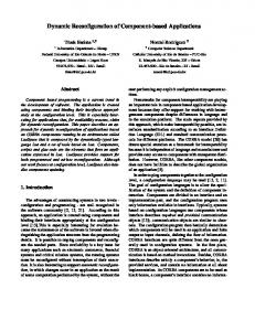
tools that enables efficient study and analysis of selected, nonquiescent scenarios in ATM networks. Accordingly, this study proposes an approach involving the use of multiresolution models to accelerate ATM network simulations to scenarios of interest. Figure 1 presents an overview of the proposed solution. As illustrated in the figure, the idea is to use a sufficiently accurate, abstract (or low-resolution), but faster model in quiescent conditions and use higher resolution models for detailed simulation when scenarios of interest appear in the simulation. The transition between the different levels of resolution is achieved using a novel methodology called dynamic component substitution (DCS). DCS enables changes to the resolution of a model by dynamically (i.e., during simulation) substituting a set of components called a “module” with a functionally equivalent component. Depending on the resolution (or details) required for the simulation study, DCS is used to dynamically change the model between the two or more configurations (as shown in Fig. 1), thereby enabling more optimal trade-offs between several modelingand simulation-related parameters. The idea is to reduce the time spent simulating inconsequential scenarios without significantly affecting the overall objectives of the simulation study. Note that, if the simulation time frames are decreased, then a number of other simulation-based analysis techniques (see section 4) will also benefit from the proposed approach. This article explores the issues involved in applying DCS to accelerate ATM network simulations to scenarios of interest. The remainder of this article is organized as follows. Brief background information on ATM networks is presented in section 2. Section 3 presents a detailed discussion of DCS. Section 4 presents an overview of some of the closely related research activities. Section 5 presents a brief overview of WESE (Web-based Environment for Systems Engineering) [9], which is a Web-based modeling and simulation framework that has been used in this article to evaluate DCS. Section 6 presents the ATM components developed using WESE’s Application Program Interface (API). A detailed discussion of the strategy employed to trigger DCS transformations inATM models is presented in section 7. Section 8 presents the statistics collated from the experiments conducted to evaluate the effectiveness of the proposed approach. The ATM network models used in this study are also presented in this section. Finally, section 9 concludes the article, summarizing the work presented. 2. Background on ATM Networks ATM is a multiplexing technology designed to be a generalpurpose, connection-oriented communication network for a wide range of services [2]. ATM networks are connection oriented because nodes on the network must establish a connection or virtual path between them to transmit data. The transmitted data are split into a number of fixed-size blocks called cells. Each cell has a fixed size of 53 octets (or bytes), which is subdivided into a 5-octet header and a

236 SIMULATION Volume 82, Number 4


ATM Cloud

ATM Cloud Client

Less details More details but Faster but Slower

S C D

S C

S

D

(scenarios of) ( interest )

C

Switches

D

S C D

High Low Resolution Resolution


Figure 1. Overview of proposed approach for asynchronous transfer mode (ATM) network simulations

48-octet payload. The cell header identifies the destination, cell type, and priority. The virtual path identifier (VPI) and virtual channel identifier (VCI) fields in the header provide necessary connection information. An ATM network is built by suitably interconnecting a set of ATM switches. An ATM switch forms the core hardware unit in an ATM network through which clients or nodes are interconnected. The ATM switch performs the following tasks: it acts as a gateway to the network; performs route discovery and management; performs creation, management, and closing of connections between clients; and performs multiplexing cells in the network. An ATM switch essentially implements the various layers of the B-ISDN/ATM protocol stack based on the International Telecommunication Union (ITU-T) and ATM forum recommendations [2, 10]. The various layers in the ATM protocol stack and their functions are shown in Figure 2. The lower-most layer in the protocol stack is the physical layer. The physical layer interfaces with the physical medium and extracts ATM cells into time division multiplexed frames that are further processed by the ATM layer. The ATM layer forms the core layer in the protocol stack. Its primary task is to perform multiplexing, switching, and control actions. The ATM layer uses the VPI and VCI fields in a cell to perform the multiplexing. In addition, the ATM layer also performs the task of interfacing with the user and other switches through the suitable user-network interface (UNI) and network-network interface (NNI). In conjunction with the management layers, the ATM layer uses the private network-to-network interface (PNNI) protocol for route discovery and management. The ATM adaptation layer (AAL) forms the top-most layer in the protocol stack. As shown in Figure 2, the AAL has two sublayers: segmentation and reassembly (SAR) and the convergence sublayer (CS). The CS is further broken down into common part (CP) and service-specific (SS) components. The AAL provides different classes of services to accommodate constant and variable bit rate traffic flowing through

the ATM network. Further details on ATM networks are available in the literature [2]. 3. Dynamic Component Substitution (DCS) DCS is a generic methodology for changing the resolution (or level of abstraction) of any hierarchical, componentbased model [9, 11]. In a component-based model, a system is represented as a set of interconnected components [9, 11]. A component is a well-defined entity that is viewed as a “black box” (i.e., only its interface and functionality is of interest and not its implementation). However, during simulation, each atomic component is associated with a logical process (LP) or a simulation object (a specific, well-defined software unit) that implements its behavior and functionality. A component could, in turn, be specified using a set of subcomponents. A set of interconnected components with a well-defined interface is called a module. A module can be viewed as a logical component. Modules are conceptual, convenient abstractions that enable development of hierarchical models and ease modeling of large systems [9]. In DCS, changes to the resolution of a model are achieved by substituting a module (i.e., a set of components) with a functionally equivalent module or vice versa. The equivalent module is chosen such that the overall characteristics of the model are not altered and deviations in the simulation results due to DCS are within acceptable limits. The equivalent module may contain one or more components. In practice, the equivalent module typically contains a single component. In such cases, the module is simply called an equivalent component. An equivalent module or component must satisfy the following criteria: 1. Interface equivalence: Equivalent modules must have an interface that is identical. The interface specification also includes the type of events that can be processed or generated by the LP associated with the Volume 82, Number 4


SIMULATION 237

Rao and Wilsey

Management Plane

Control Plane

User Plane

Convergence Sublayer (CS)

Service Specific (SS)

Segmentation & Reassembly (SAR) Sublayer [Generic Flow Control] [Call Header Generation/Extraction] [Cell VCI/VPI Translation] [Cell Multiplexing/Demultiplexing]

ATM Layer

Physical Layer

Common Part (CP)

Layer Management

ATM Adaptation Layer

Higer Layers

Plane Management

Higer Layers

Transmission Convergence (TC) Sublayer [Cell Rate Decoupling, Cell Delineation] [Transmission Frame Generation, Adaptation, & Recovery] Physical Medium (PM) Sublayer [Bit timing, physical medium]

Figure 2. Overview of B-ISDN/ATM protocol stack (ITU-T & ATM Forum standard)

component. The interface equivalence property ensures that DCS transformation occurring to a module is completely transparent to any other interconnected component. 2. Functional equivalence: The equivalent modules must have similar functionality, as defined by the modeler. In other words, the behavior and functionality of a given pair of equivalent modules need not be identical but within acceptable limits. This flexibility enables the application of different forms of abstractions to the model. This criterion is a weaker requirement than the interface invariance property. Substitution of components may be done statically or dynamically. Static abstraction occurs during model development or prior to commencement of simulation. Static component substitution is widely used in different flavors to address capacity and performance issues of large-scale simulations [12, 13]. The primary drawback of the static methods is that the trade-off between fidelity, resolution, and simulation overheads cannot be altered during simulation. On the other hand, substituting components during simulation provides a dynamic trade-off between the modeling- and simulation-related parameters. Dynamic flavor of DCS can be further classified into the following categories: Proactive DCS: Approaches in which DCS transforma-

tions are scheduled to occur in the future (with respect to simulation time) are classified as in the proactive strategies. Proactive strategies are used when the scenarios for triggering DCS are known a priori. Typically, such strategies are used to drive the model to configurations that are known to improve performance. However, detecting suitably scenarios and triggering proactive transformations can be a complex task. Reactive DCS: In reactive strategies, DCS transformations are scheduled at the current simulation time or in the past. A number of approaches can be adopted for achieving changes in the past. For example, a check-pointing and rollback mechanism can be used to restore an earlier state of the simulation and perform the DCS transformations. Reactive strategies are used to detect and recover from possibly incorrect or inefficient proactive transformations. Typically, detecting scenarios requiring reactive transformations is easy. However, providing the simulation infrastructure for reactive transformations can be a complex task. DCS can be used to enable more optimal trade-offs between several modeling, simulation, andV&V (verification and validation)–related parameters. This study uses a combination of proactive DCS abstraction and reactive DCS refinement of the model to accelerate ATM simulations. Furthermore, DCS enables effective “what-if” analysis and exploration of design alternatives to be carried out during the lifetime of a simulation by striking a dynamic trade-




off between resolution, fidelity, and performance [14]. It is also an attractive solution to accelerate rare event simulations [6]. In addition, DCS is an effective technique for enabling large-scale simulations [15]. It can also be used to ease debugging by rapidly accelerating simulations to scenarios of interest [6]. It enables more thorough validation of simulations by analyzing the model at different levels of abstraction [6]. However, analogous to any multiresolution approach, care must be taken when applying DCS to avoid several modeling and simulation pitfalls, such as temporal inconsistencies, ghosting of attributes, high transition latency, thrashing, and degradation in fidelity [6, 16]. One of the most attractive and important aspects of DCS is that an algebra has been developed about a mathematical framework for reasoning about the changes induced in the model by DCS transformations [17]. The algebra has its foundations in discrete mathematics and set theory. The algebra clearly defines and delineates the various transformations that can be induced in the model. Based on the axioms underlying the algebra, it has been proven that a sequence of DCS transformations satisfies properties of closure, associativity, inverse, and identity, thereby making DCS transformations a “group” (in discrete mathematics) [18]. In other words, DCS is not an ad hoc approach. Moreover, a number of discrete mathematics tools and laws can be applied to further extend and ease mathematical analysis. For example, if all the transformations are unique (i.e., the set of components of modified various DCS operations does not overlap), then it can be shown that the set of transformations forms an Abelian group [18]. In addition, statistical extensions to DCS algebra have been employed to develop a DCS performance prediction methodology (DCSPPM). DCSPPM provides quantitative estimates of the performance changes induced by DCS [17, 19]. The quantitative estimates enable a modeler to identify optimal, dynamic model configurations prior to simulation [19]. These aspects make DCS a rigorous and efficient approach for performing multiresolution simulations. Further details on DCS are available in the literature [6, 15, 17, 20]. 4. Related Research This work addresses two broad areas—namely, multiresolution modeling and simulation of ATM networks. DCS is an alternative approach for multiresolution modeling and simulation. The context (or application domain) of this work is accelerating the simulations of ATM networks to nonquiescent conditions. A brief overview of only the most closely related research activities is presented in the following subsections because a detailed literature survey of these broad areas is beyond the scope of this article. Readers are referred to the literature for further references. Section 4.1 presents some related research in the domain of dynamic resolution simulations, in which the level of abstraction of the model varies during the course of simulation. Some of the related research in the field of ATM network simulations is presented in section 4.2.

4.1 Dynamic Resolution Simulations A number of studies have been reported on selectively abstracting parts of a model to enable efficient trade-offs between several model- and simulation-related parameters. However, many of the studies involve static abstractions that are preformed prior to commencement of simulation, which is not the context of this work. This study deals with dynamically (i.e., during simulation) changing the resolution of the model, and only those investigations relevant to this work are briefly described in this section. Ahn and Danzig [21] have demonstrated that abstraction can be employed to adjust the simulation granularity of packet network models to efficiently study flow and congestion control algorithms. Their work deals with dynamically combining a cluster of closely spaced packets into a train and operating on the train rather than individual packets. In this research, we dynamically abstract or refine ATM subnets to accelerate the simulation. Hybrid simulation models, wherein the network model is a combination of discrete event and analytical components, have been used to yield efficient yet accurate simulations [22]. Davis and Hillestad [23] present a discussion on applying variable resolution modeling (VRM) techniques to the domain of military models. Their work deals with applying VRM to military models, while this work deals with ATM network simulations. Lee and Fishwick [24] discuss a taxonomy for abstraction of dynamic systems through structural simplifications, behavioral approximations, and data abstraction. This research deals with dynamically selecting appropriate equations to represent characteristics of a system as simulation progresses and the system’s state changes. On the other hand, this research deals with dynamically changing the components constituting the model, specifically in the domain of ATM networks. One of the closest research activities related to DCS is by Natrajan, Reynolds, and Srinivasan [25] and Reynolds, Natrajan, and Srinivasan [16]. They propose the use of multiple resolution entities (MRE) to enable dynamic changes to the abstraction or resolution of a model. They provide a framework for maintaining consistency across multiple levels of resolution, using an MRE that can be developed. They present some of the issues such as ghosting, chain disaggregation, and network flooding to motivate their approach. In MRE, all desired levels of resolution are conceptually active throughout the simulation. Contrarily, in DCS, only one level of abstraction is active at any given point in simulation time. We believe that maintaining only a single level of abstraction is critical for achieving high performance. MRE does not deal with changing or triggering changes in resolution because the various levels are concurrently maintained. On the other hand, DCS has an explicit concept of triggering transformations in a proactive or reactive manner. An MRE component typically has multiple interfaces at different levels of resolution. Conversely, in DCS, a component has only a single interface exposed for model development. Leveraging the premise Volume 82, Number 4


SIMULATION 239

Rao and Wilsey

of a single interface, we have developed a DCS algebra based on set theory and discrete mathematics. The DCS algebra provides a more robust framework for mathematical analysis of DCS [6]. Furthermore, component-based modeling using single interfaces yields itself to V&V using the formal software engineering and automated theorem, proving Rao [6]. Last but not the least, we have developed a sophisticated DCSPPM for predicting changes in simulation performance due to DCS [19]. DCSPPM enables effective use of DCS by identifying performance-improving transformations prior to simulation and selectively applying those transformations [6, 19]. We believe these aspects are crucial for the successful use of dynamic resolution models and simulations. These aspects significantly differentiate DCS from all of the earlier investigations in the area of dynamic resolution modeling. 4.2 ATM Network Simulations The steady advancement in technology coupled with growing needs and demands has resulted in significant concerns about QoS of broadband and telecom networks [7]. The primary challenges in evaluating today’s networks are stringent limits on QoS requirements, network performance, increasing size and complexity, tight logical coupling between subsystems, and cost versus time trade-offs. In an endeavor to meet the growing need for cost-effective yet accurate analysis of ATM networks, several approaches have evolved in the recent past. The approaches used for analysis of broadband and telecom networks can be broadly classified into three categories—namely, (1) analytical methods, (2) emulation or direction measurement approaches, and (3) simulation-based methods. The analytical methods are typically used to analyze quiescent condition of networks. Analytical methods represent the desired aspect of the network under study using mathematical equations. A variety of mathematical tools are employed to solve the set of equations to yield various system properties. This approach can be very efficient. However, the primary drawbacks are that it requires a high level of abstraction, considerable effort and skill, and considerable knowledge of the system. The complexity of today’s networks makes this a formidable and, in many cases, an impossible task without unrealistic assumptions [7]. In the emulation or direct measurement approaches, an existing system or a prototype is used to perform experiments, and the results obtained are extrapolated to predict the performance of the target system. One of the primary drawback of this techniques is that considerable investment is required for the analysis to be effective. Furthermore, it does not scale for analysis of large systems. However, it is effective for testing and analysis of small systems under development [7]. This research does not deal with analytical techniques or emulation-based methods. Consequently, these topics are not explored in this article. To circumvent the shortcomings of analytical techniques and emulation-based approaches, experimental

methodologies such as computer-based simulations are widely used. The primary advantage of simulations is that they can be used to analyze new systems. In addition, simulations enable exploration of scenarios that would otherwise be impossible to analyze. Furthermore, simulation is nondestructive and a cost-effective approach. To enable rapid analysis, simulation-based approaches usually strike a trade-off between a number of factors such as nature and type of model used, the nature and type of input vectors used, and space versus time trade-offs when distributed computing techniques are employed. One of the common approaches to accelerate analysis using simulation-based techniques is to decompose the model into submodels such that the submodels are analytically tractable. The submodels are analyzed using analytical techniques while the system as a whole is studied using simulations. Ammar and Deng [26] have shown that the application of time scale decomposition in conjunction with Time Warp–based parallel simulations can improve performance of simulations. The drawback of time scale or spatial decomposition is that it is very specific to the system under study and requires system expertise. Furthermore, several restrictive assumptions must be placed on the model to allow decomposition [7]. In contrast, the proposed methodology does not make any restrictive assumptions and is broadly applicable to various configurations of ATM networks. A number of statistical techniques have been proposed to analyze the results obtained from the simulations. Statistical techniques are used to reduce the variance in observations, using fewer simulation runs or data points. The use of antithetic sampling using correlated samples is discussed by Heegaard [7].An alternative technique is to use common random numbers on two similar models and use some comparative performance measures such that the full system will have reduced variance if the two models are synchronized. Alternatively, control variables are used to isolate the influence of variables on the system. However, several representative statistics are required for applying statistical techniques. Schormans et al. [27] present a hybrid technique involving the use of mathematical techniques to represent background traffic and use cell simulations only for foreground traffic, thereby accelerating ATM simulations. A recent dissertation discusses the use of static multiresolution network models that use a combination of fluid and packet flow models to accelerate simulations [28]. Villén-Altamirano [29] proposes the use of the RESTART approach to improve the occurrence of rare events in simulations. The basic idea underlying the RESTART approach is to sample the rare events from a reduced state space where this event is less rare. In this approach, a simulation is initially driven close to the scenario of interest. The probability of the reduced state space occurrences is estimated by direct simulation and by using the Bayes formula to determine the final value. The RESTART approach can be implemented in different ways. Gorg and Schreiber [30] present the use of the limited relative error




(LRE) technique in conjunction with RESTART to control variability and improve convergence. Villén-Altamirano [29] presents further extensions to the RESTART method in which multiple initial states are used to analyze the probability of occurrence of another state. Kuhlmann and Kelling [31] present case studies on applying multidimensional RESTART simulations. L’Ecuyer and Champoux [32] discuss simulation-based techniques for estimating cell loss ratios in an ATM switch using queuing network models. They present the use of importance sampling to improve the efficiency of their simulations. Parallel and distributed simulation techniques are employed to reduce the time for simulation. One approach is to run multiple, concurrent simulations using a sharedmemory multiprocessor or a distributed network of workstations. An earlier research activity by Lamers and Gorg [33] employs this approach. Alternatively, parallel simulation techniques are used to run a given simulation using multiple processors to reduce simulation time frames. Bhatt et al. [34] present parallel simulation techniques based on Time Warp simulations to accelerate simulation of ATM network models developed using the Telecommunications Description Language (TeD). Pham and Fdida [35] present the issues involved in cell-level simulation of large ATM networks using a conservatively synchronized parallel simulation kernel.

(SSL). The specification of a model or an SSL design file consists of a set of interconnected modules. Each module consists of three main sections—namely, (1) the component definition section that contains the details of the components to be used to specify a module (such as the Universal Resource Locator [URL] of a factory and name of the source object along with initial parameters), (2) the component instantiation section that defines the various components constituting the module, and (3) the netlist section that defines the interconnectivity between the various instantiated components. SSL permits an equivalent component to be associated with each module. DCS is performed by replacing the module with its equivalent component or vice versa. SSL also allows an optional label to be associated with each module. The label can be used as a component definition in subsequent module specifications to nest one module within another. This technique can be employed to reuse module descriptions and develop hierarchical specifications. The input SSL source is parsed into an objectoriented (OO) in-memory intermediate form (SSL-IF). Hierarchical SSL models are elaborated or “flattened” prior to simulation by the elaborator [9]. Elaboration is a recursive process that flattens a hierarchical model by substituting each module reference (made through the use of labels) with an unique instance of the module.

5. Web-Based Environment for Systems Engineering (WESE)

5.2 Simulation Subsystem

This section presents a brief overview of WESE [9, 15, 17], which is used later in this article for the performance studies. An overview of WESE is shown in Figure 3. As illustrated in this figure, WESE has been developed using a set of well-defined, asynchronous, interacting, and coordinated subsystems and modules. Each subsystem or module provides a well-defined and robust interface for configuration, interaction, coordination, monitoring, and control. Such a modular design philosophy has been motivated by the need to address several abstract but important aspects of WESE, such as ease of design and implementation, maintainability and troubleshooting, adaptability for future enhancements, robustness or fault tolerance, separation of concerns, ability to interface with third-party subsystems, and to ease “plug-and-play” of subcomponents. WESE provides a component-based modeling language, a framework for developing a Web-based repository of components, and the infrastructure for DCS-capable distributed simulation. The following subsections present the modules and subsystems constituting WESE in more detail. 5.1 Modeling Frontend WESE provides both an HTML interface and a text-based frontend that can be used to interact with the WESE server (Fig. 3). The primary input to WESE is the model of the

system described using the System Specification Language

The core module of WESE is the server (Fig. 3). The WESE server performs the task of collaborating with the distributed factories and coordinating the simulations. The factory manager performs the tasks of interacting with the distributed WESE factories using a predefined protocol. A WESE factory can be viewed as a Web-based repository of components with added capability to simulate them. Parallelism occurs at the factory level (i.e., each factory is a parallel, asynchronous simulation infrastructure) [9]. Parallel simulations are performed by using components (or simulation objects) from different factories. A WESE factory is built from subfactories and object stubs. Object stubs contain attributes of the a component such as interface description, cost, and formal specifications. 5.2.1 WARPED The simulation subsystem of a WESE factory has been developed using the WARPED simulation kernel. WARPED is an API for a general-purpose discrete event simulation kernel with different implementations [36]. WESE uses the time warp–based [36] simulation kernel of WARPED. A Time Warp synchronized simulation is organized as a set of asynchronous logical processes (LPs) that represent the different physical processes being modeled. The LPs exchange event information by exchanging virtual timestamped event messages. Virtual time [37] is used to model the passage of time and defines a total order on the events in

Volume 82, Number 4


SIMULATION 241

Rao and Wilsey

Web−Based Environment For Systems Engineering

WESE Simulator

Factory

Factory

Client’s Browser

Model SSL

Simulator

WESE−FVF Server HTML (CGI) Pages

SSL−IF Factory

SSL Parser & Elaborator

Manager

Factory

Reports Text Interface Front End/ Interface

Theorem Prover

Simulation Manager

System Requirements (User)

DCSPPM Module

Information Manager

Simulator

Specification Generator

Legend Communication Sub−System

(PVS) Generated Spec.

Figure 3. Overview of WESE

the system. Each LP processes its events by incrementing a local virtual time (LVT), changing its state, and generating new events. Although each LP processes local events in their correct time stamp order, events are not globally ordered. Causality violations are detected when an event with time stamps lower than the current LVT (a straggler) is received. On receiving a straggler event, a rollback mechanism is invoked to recover from the causality error. The rollback process recovers the LP’s state prior to the causal violation, canceling the erroneous output events generated and reprocessing the events in their correct causal order. Each LP maintains a queue of state transitions along with lists of input and output events corresponding to each state to enable the recovery process. A periodic garbage collection technique based on global virtual time (GVT) is used to prune the queues by discarding history items that are no longer needed. The distributed simulation is deemed to have terminated when all the events in the system have been processed in their correct causal order. A more detailed description of WARPED, Time Warp, and WESE are available in the literature [36, 38]. 5.3 Infrastructure for DCS The modeling and simulation subsystems of WESE provide the infrastructure for enabling both proactive and reactive DCS. SSL includes the necessary language constructs for modeling, the factories provide infrastructure

for component development, and the simulation subsystem performs the core tasks involved in enabling DCS. In WESE, an event-driven mechanism has been employed to sequence the various phases involved in DCS [39]. This approach makes the DCS implementation immune to the idiosyncrasy of the synchronization mechanism. A component can trigger DCS by merely scheduling an appropriate kernel event. The DCS infrastructure of WESE provides support for both proactive and reactive transformations. Proactive DCS transformations occur in the future with respect to simulation time. Such transformations have been enabled by using the standard simulation infrastructure of WARPED. Special kernel events are scheduled to trigger proactive transformations. WESE provides API calls to schedule proactive DCS transformations to occur in the future. On the other hand, enabling reactive DCS transformations is more involved. In WESE, reactive DCS has been enabled by using the built-in state-saving and rollback mechanism provided by the Time Warp kernel of WARPED. Reactive DCS transformations are achieved by artificially rolling back the simulation to an earlier simulation time (i.e., earlier than the time when the transformation needs to occur) and then performing the DCS transformation. The overheads of rollbacks and causal consistency maintenance are transparent to the application. To enable reactive DCS, the state of the simulation at the desired time needs to be available. To ensure that the states are available, WESE provides suitable API calls that can be used to delay fossil collection in the




simulations. Care must be taken to ensure that an optimal value is specified so that the memory usage of the simulation does not significantly increase. The delayed fossil collection can be enabled and disabled by the application during the course of the simulation. In addition, WESE also provides an API and infrastructure for mapping states of components during DCS. 5.3.1 Error Propagation Library (EPL) WESE also includes a lightweight Error Propagation Li-

brary (EPL) that provides a set of statistical functions that can be used to track and propagate errors in simulation results that may arise due to DCS transformations. In conjunction with WESE, it has been developed in C++. The object-oriented features of C++ have been used to seamlessly integrate EPL with the modeling and simulation infrastructure of WESE. For each basic numeric data type in C++ (such as int, float, and double), the EPL defines a corresponding data type (such as INT, FLOAT, and DOUBLE). Each EPL data type maintains the numerical data in the form x ± ∆x, where x is the default value (that would be maintained if EPL is not used), and ±∆x represents the error or uncertainty in the value of x [40, 41]. EPL provides a number of statistical functions that can be used to determine the uncertainty or errors. In addition, operator overloading has been used to define suitable mathematical operators for the EPL values. The operators suitably propagate the uncertainties across mathematical operations. The EPL values can be seamlessly used in simulation events, and they automatically propagate uncertainties through the model. Careful use of EPL can significantly increase confidence in the results obtained from simulations without significantly affecting overall simulation performance. 6. ATM Factory: Set of ATM Components As explained in section 5, models are developed by collating a set of components into a WESE factory and using SSL to develop the models by suitably interconnecting components. This approach is commonly used in other simulation environments as it provides flexibility and increases reusability of components. A set of typical ATM networking components has been developed and bundled into an ATMFactory. The components have been developed to provide sufficient flexibility so that their working can be fine-tuned using suitable parameters (in the SSL description). Care has been taken to ensure that the overall organization of the model and components closely reflects their real-world counterparts. The ATMFactory provides a PMLayer and TCLayer component that are used to model the physical layer of an ATM switch (Fig. 2). The PMLayer component must be used to send and receive data between any two nodes in the simulated ATM network. In addition to transmitting and receiving data, this layer also provides primitives for latency detection and bandwidth negotiations between ATM

switches. The TCLayer component models the transmission convergence sublayer. It generates suitable header error correction (HEC) for the incoming and outgoing ATM cells and performs necessary validation. This component forms the link between an ATM layer component and a PM component within an ATM switch. The ATM layer is the core of an ATM switch and performs a diverse set of functions. Consequently, the ATM layer component has been modeled using a set of C++ classes with suitable APIs. The idea is to provide a flexible and extensible infrastructure for further development. The set of components constituting the ATM layer (AL) performs the following diverse functions: 1. PNNI-Related Functions: The AL component handles all the signals and activities related to the PNNI of ATM networks. Currently, point-to-multipoint call and connection controls are not supported. Call creation includes parameters for specifying the desired bandwidth, latency, and jitter. This component also performs the tasks related to PNNI-based routing such as route discovery and routing table distributions. The AL component supports a weighted shortest path routing mechanism for route discovery, where weights are computed based on the bandwidth of the links. TheAL component indirectly uses the PM component to negotiate and determine bandwidth of the links. Routes are periodically refreshed to check and recover from link failures. 2. VCI/VPI Translation: The AL component maintains a table of active VCI and VPI at each ATM switch. The AL component translates and multiplexes each ATM cell from one VCI to another using an activity indicator for each VCI. The AL chooses a suitable time slot for transmitting a cell based on the traffic contract for a VPI. Remaining cells are rescheduled to be transmitted at a later simulation time. This approach is a trade-off between the amount of memory required for maintaining large ATM memory buffers versus rescheduling overheads. In addition to the above components, the ATMFactory also provides traffic generators that can be configured as servers or clients. The clients also include a suitable abstraction of the ATM adaptation layer (AAL). The traffic generators provide parameters for configuring the type, volume, and rate at which they generate ATM cells along with sources and destinations (specified as 64-bit hierarchical ATM addresses). The generators provide statistical distributions and a Markov-modulated Poisson process (MMPP)–based mechanism for generating ATM traffic. 6.1 ATM Cloud The ATM Cloud (AC) represents a higher level abstraction (or lower resolution) of a set of interconnected ATM Volume 82, Number 4


SIMULATION 243

Rao and Wilsey

ATM Switch

DCS

ATM Cloud ( Single Component or ) (Logical Process [LP] ) Client Component

Client Component

Ports

Simulation Configuration #1

ATM Cloud

(a) Simulation Configuration 1

Simulation Configuration #2 (b) Simulation Configuration 2

Figure 4. Overview of implementation of dynamic component substitution (DCS) in asynchronous transfer mode (ATM) models

switches (see Fig. 4). The ATM Cloud is also an integral part of the ATM Factory. The AC essentially represents an ATM subnetwork. Multiplexing of cells within the AC proceeds at a much faster rate because intermediate cells are not generated. Instead, an incoming cell is directly multiplexed onto an outgoing link. However, it must be noted that theAC does not perform any task (such as PNNI signaling, etc.) other than multiplexing cells. The AC multiplexes cells, using a given set of VC tables. The VC tables are obtained from various AL components encapsulated by an AC. The VC table information stored in the state of each AL component is passed to the corresponding AC when proactive abstraction is triggered. The AC uses the VC table information and updates its internal state during the abstraction process. When a cell arrives at a port, the AC uses the VC table corresponding to that port to determine information about the next hop. If the next hop is to an AL component within the AC, it looks up the appropriate VC table for further multiplexing information. On the other hand, if the next hop lies outside the AC, it generates a new cell event with appropriate delays (computed as discussed in the next paragraph) and schedules the event. The AC component uses a more straightforward approach to determine cell delays when compared to the AL components. The AL components strive to minimize jitter by applying realistic cell multiplexing behaviors. On the other hand, the AC simply uses the maximum acceptable jitter value. The motivation for a more straightforward approach is to minimize state information in the AC. To achieve realistic multiplexing behaviors, the AL components maintain detailed cell transmission schedules for each outgoing link in their state. The state information is typically small because of the few number of links on each AL. However, an AC contains several AL layers, and maintaining detailed cell transmission schedules for each AL significantly increases the state size and state-saving overheads. To minimize state overheads, the AC simply uses the

maximum acceptable jitter values for links encapsulated by the AC and does not perform detailed cell scheduling like the AL layers. Consequently, deviations in cell timings may occur when cells are multiplexed by an AC component rather than by an AL component. Note that the upper bound for these deviations is the maximum jitter value for a given VC. To validate the timings obtained from simulations involving DCS, the AC sets a suitable variation (±n microseconds) in timings along with the cell. The variances are tracked and errors are propagated using WESE’s EPL (section 5.3.1). The objective is to ensure that the jitter and delays provided by the AC are comparable to that of the ATM switches, thereby increasing the confidence in the results obtained from simulations. The AC component assumes that abstraction occurs only when the traffic on various links is below a certain threshold and all the traffic can be accommodated without any cell loss. Currently, the threshold is set to 85% bandwidth of the slowest link associated with an ATM cloud. If the traffic exceeds 85% of the bandwidth, then it is assumed that cell loss may occur and abstraction is inhibited, thereby forcing high-resolution simulations. Accordingly, the AC does not check for cell loss but reactively refines the model when any traffic other than ATM cells are received. Refer to section 7 for details on the DCS strategy used in this study. The AC multiplexes cells at a much faster rate than a set of ATM switches. For example, consider a case shown in Figure 4, in which four ATM switches are encapsulated into an ATM Cloud. On a 2-GHz Athlon XP processor, the wall clock time to multiplex a cell through the AC is about 4 (±0.25) microseconds, while multiplexing the cells through four individual ATM switches (consisting of AAL components, ATM components, TC components, and PM components) takes 60 (±0.63) microseconds. In other words, the AC component is faster than a set of ATM switches by more than 10 times. The primary factor con-




tributing to the performance improvement is the elimination of intermediate simulation events and corresponding simulation overheads (such as event creation, scheduling, and event processing) for multiplexing the cell across each individual ATM switch. In the proposed study, DCS is used to abstract and refine a subnetwork by substituting a set of ATM switches (highresolution entities) with an ATM Cloud (low-resolution entity). During DCS, the states of the various components (such as AAL components, ATM components, and PM components) are mapped to the corresponding ATM Cloud component using suitable API methods. The state mapping provides information about the active channels (VPI, VCI, and traffic contract) along with other information on each ATM switch. Note that the set of components encapsulated by an ATM switch is automatically determined (from the SSL description) and maintained by WESE. In addition, WESE also handles the issues involved in properly routing events between components when DCS occurs. 7. Strategy for DCS A brief overview of the proposed solution to accelerate ATM network simulations using DCS was discussed in section 1. Figure 4 presents an overview of the implementation. The proposed solution has been implemented in the simulations as follows. As shown in Figure 4, the module (set of components) undergoing DCS in an ATM network model is an ATMCloud. The ATMCloud encapsulates a number ATMSwitches. As shown in Figure 4, each ATM Switch further encapsulates other components, depending on the number of physical connections to the switch. DCS is performed by substituting a set of ATMSwitches (Fig. 4(a)) with a corresponding ATMCloud (Fig. 4(b)) in the following fashion: • The simulation starts off at the highest resolution (lowest level of abstraction). DCS is inhibited for first few seconds (simulation time) of network activity. DCS is inhibited because during the first few seconds, the network remains in a nonquiescent condition as traffic negotiations are performed, routes between ATM switches are being established, and the clients create new connections. The duration of the startup phase depends on the size of the network. Currently, the duration of the startup phase is specified by the model developer. • Once the initial startup phase has been completed, the ATMCloud periodically triggers proactive abstraction. Proactive abstraction is speculatively triggered with the assumption that the network has reached a stable condition. Furthermore, abstraction of a subnet is inhibited when the traffic on the subnet is high (more than 85% of a link’s bandwidth) and the probability of cell loss is high. In addition, the abstract ATMCound components assume that abstrac-

tion occurs only when links are not heavily loaded and do not perform checks for cell loss. • Whenever the ATMCloud receives an event other than a ATMCell (say an ATMSignal), it triggers a reactive refinement of the model. The simulation is rolled back to the time when the event was generated. The model is refined, and the simulation proceeds at a higher resolution. The ATMCloud schedules itself an event into the future to check and trigger proactive abstractions. Note that the difference in simulation times when an event is generated and when the same event is received is determined by the delay of the link on which the event logically traverses. Consequently, the maximum rollback distance of an ATM Cloud is the delay of the slowest link connected to it. However, to enable rollbacks, the simulator needs to maintain one state prior to the rollback time [36]. Accordingly, to enable reactive refinement, the GVT value is throttled by two times the slowest link associated with any ATMCloud component in a model. Throttling the GVT in turn delays fossil collection in the simulation, thereby providing the necessary state information needed for reactive refinement. Given an upper bound on the reactive rollback distance and corresponding throttle value for GVT, the simulation will never roll back before GVT. Currently, it is the modeler’s responsibility to determine the slowest link and specify that value in the model description. • Due to the type of multiplexing adopted in the implementation, the ATMLayer may receive ATMSignals while the model is in its abstract state. In such cases, the ATMlayer component triggers a reactive refinement so that the signals can be processed correctly. As required by WESE’s API, the various components override the serialize and deSerialize API methods to map the current state of the various components. When abstraction occurs, each ATMLayer component dispatches its connection table and activity indicators to the enclosing ATMCloud. On the other hand, when refinement occurs, the ATMCloud dispatches the activity indicators to corresponding underlying ATMLayer components. Since the ATMCloud does not process signals, it cannot induce any change in the connection tables. Consequently, the ATMCloud does not redistribute the connection tables and avoids unnecessary state-mapping overheads. SSL’s elaboration module and WESE’s API provide the necessary information for achieving the mapping efficiently. 8. Experiments The experiments conducted to evaluate the effectiveness of applying DCS to ATM network simulations were conducted using a set of ATM network models. The basic ATM Volume 82, Number 4


SIMULATION 245

Rao and Wilsey

(* SSL description of an ATMSwitch module *) ATMSwitch2(2, 2) { ComponentDefinitions { (* This section defines the type of components used in the ATM Switch *) ATMLayer(2, 2) : localhost:2022.ATMFactory.ATMLayer "--ports 2" others; : localhost:2022.ATMFactory.TCLayer; : localhost:2022.ATMFactory.PMLayer "--inport 2" others;

TCLayer(2, 2) PMLayer(2, 2)

} ComponentInstantiations { (* Component Instantiation Section *) atm : ATMLayer; tc1 : TCLayer; tc2 : TCLayer; pm1 : PMLayer "--atm-port-id 1 --bandwidth 155.52"; pm2 : PMLayer "--atm-port-id 2 --bandwidth 155.52"; } Netlists { tc1(OUT, 1) : atm(IN, 1); atm(OUT, 1) : tc1(IN, 1); pm1(OUT, 1) : tc1(IN, 2);tc1(OUT, 2) : pm1(IN, 1); pm1(IN, 2) : ATMSwitch2(IN, 1); pm1(OUT, 2): ATMSwitch2(OUT, 1); tc2(OUT, 1) : atm(IN, 2); atm(OUT, 2) : tc2(IN, 1); pm2(OUT, 1) : tc2(IN, 2); tc2(OUT, 2) : pm2(IN, 1); pm2(IN, 2) : ATMSwitch2(IN, 2); pm2(OUT, 2): ATMSwitch2(OUT, 2); }

(* SSL description of an ATM sub-network *) (* with 3 switches. *) ATMSubNet(2, 2) : localhost:2022.ATMFactory.ATMCloud "--ports 2 --switches 3 --dcs-start-time 220000 " "--gvt-delay 13.75" others { ComponentDefinitions { (* We don’t have any component definitions here. *) } ComponentInstantiations { switch1 : ATMSwitch2 "--address-1 0.0.0.0.0.0" others; switch11: ATMSwitch2 "--address-1 0.0.0.0.0.1" others; switch12: ATMSwitch2 "--address-1 0.0.0.0.0.2" others; } Netlists { switch11(OUT, 1): switch1(IN, 1); switch1(OUT, 1) : switch11(IN, 1); switch11(OUT, 2) : ATMSubNet(OUT, 1); switch11(IN, 2) : ATMSubNet(IN, 1); switch12(OUT, 1) : switch1(IN, 2); switch1(OUT, 2) : switch12(IN, 1); switch12(OUT, 2) : ATMSubNet(OUT, 2); switch12(IN, 2) : ATMSubNet(IN, 2); } }

}

(a) ATM Switch module

(b) ATM Cloud module

Figure 5. Hierarchical System Specification Language (SSL) description for an asynchronous transfer mode (ATM) network model. (a) ATM switch module. (b) ATM cloud module.

components available in the ATMFactory have been used in a hierarchical manner to develop the network models. The basic modules in the network models are ATMSwitch and ATMClient. Figure 5(a) presents the SSL description for an ATMSwitch with two ports. Each input-output port pair is indirectly connected to a single ATMLayer component via a PMLayer component and a TCLayer component. The PMLayer components form the primary input and output components of the ATMSwitch module. Suitable parameters are provided to the various components. In addition, as shown in Figure 5, SSL’s “others” clause has been used to pass in hierarchical parameters (such as ATM addresses, etc.) from higher level module instantiations down to the final component instantiations. In the next hierarchical level, a set of ATMSwitch modules is suitably interconnected to form a subnetwork, as shown in Figure 5(b). The subnetwork is the higher resolution equivalent of an ATMCloud. Accordingly, as shown in Figure 5, suitable equivalent component specifications are provided for the subnetwork modules using an ATMCloud component. The parameters necessary to customize the working of the ATMCloud are also provided. For instance, the delay in GVT to throttle fossil collection to enable reactive rollbacks is specified using the --gvt-delay parameter. The value for GVT delay is determined based on the fact that the slowest link to the cloud is a 64-MBPS link. That implies that an 55-octet ATM cell will have a delay of (55 ∗ 8)/(64 ∗ 106 ) = 6.875 µsec on this link. In other words, an ATMCloud component would have to roll back 6.875 µsec in simulation time when reactive refinements occur. However, as discussed in

section 6.1, the simulator needs to maintain one state prior to the rollback time to enable rollbacks [36]. Based on this information, the GVT delay for this model has been set to 6.875 ∗ 2 = 13.75 µsec. Using a similar procedure, ATM network models have been developed to empirically evaluate the effectiveness of the proposed approach. The salient characteristics of the models are shown in Table 1. The vBNS+ example shown in Table 1 is a model of the very high-performance Backbone Network Service (vBNS+) that has been under development since 1995 [42]. The network topology of vBNS+ is shown in Figure 6. It now provides a nationwide, high-performance ATM backbone for IP over ATM-type applications that require highperformance and high-bandwidth networking. vBNS+ has been developed through a cooperative agreement between MCI and the National Science Foundation (NSF). The primary traffic on the vBNS+ backbone is IP over ATM generated by edge IP routers connected to an ATM switch. The edge routers are modeled using an ATMIPClient from the ATMFactory. Based on some of the statistics available off the Internet, the clients were programmed to choose a random destination, establish connections to it, download a few megabytes of data, and close the connection. Each client typically has four to eight concurrent connections open. This scheme reflects the “typical” behavior of an edge router in the vBNS+ backbone. Care was taken to appropriately seed the random number generators so that the experiments were repeatable. The vBNS+ model also includes an Address Resolution Protocol (ARP) service. It has been developed to resolve IP address to ATM addresses for this application. The ARP tables are manually provided




Table 1. Characteristics of the ATM models Model Name

Normal

Number of Components Abstract

Total

Hierarchies in Model

vBNS+ ATMNet1 ATMNet2

241 1495 1495

4 27 27

245 1522 1522

4 5 5

ATM Clouds

Seattle C

Boston C

Ameritech NAP C C

C

San Francisco

A

C

Denver

J

C

C

A

Chicago Cleveland C A Pittsburgh NCSA C Washington DC

C

New York C

C Sprint NAP

C Perryman C

C MFS NAP

Los Angeles

C J

C C

A

Atlanta

San Diego

A − Ascent GRF 400 C − Cisco 7507 C − Cisco 12008 J

− Juniper M40

− Fore ASX−1000 − NAP

C

Houston

− OC−3C − OC−12C − DS−3

Figure 6. Topology of vBNS+ model

(through a data file), and the ARP service uses these data for resolving addresses. The vBNS+ model has been developed in a hierarchical fashion by describing the network topology in SSL. As indicated in the column titled “Hierarchies in Model” in Table 1, the vBNS+ model contains four hierarchical levels. The top-most hierarchical level consists of a set of edge routers connected to four ATM clouds. Figure 6 illustrates the four clouds. The clouds have been defined based on their geographic locations. The four ATM clouds form the next tier in the hierarchical model. Each cloud has a corresponding ATMCloud component associated with it. The number of such abstract ATMCloud components in

each model is tabulated in Table 1, in the column titled “Abstract.” Each cloud encapsulates a set of ATM switches and links that constitute the third hierarchical level. Each ATM switch in turn consists of one ATMLayer component and several TCLayer and PMLayer components that constitute the lowest level in the hierarchy. The number of these atomic components, along with traffic generators and clients in each model, is shown in the column titled “Normal” in Table 1. Note that, as illustrated in Figure 6, each ATMCloud encapsulates a different number of ATM switches. At any given point in the simulation, zero or more of the ATMCloud components are active, and the components encapsulated by it Volume 82, Number 4


SIMULATION 247

Rao and Wilsey

are inactive (or vice versa) due to DCS transformations. Accordingly, as the number of active ATMCloud components increases, the total number of active components in the simulation decreases. The clients and traffic generators in the model are always active and are not affected due to DCS transformations. Note that ATMCloud components cannot be nested within each other. The ATMNet1 model has been developed by suitably adapting an ATM network model developed by Perumalla and Fujimoto [43] at Georgia Tech. The model has also been used by other researchers for study and analysis of ATM networks [34]. The traffic in this example is pure ATM-type traffic generated by the clients. The clients generate a constant bit rate–type traffic (typical to voiceover ATM/Sonet-type applications) with some acceptable (prespecified) jitter [1]. Each client has only one connection active at a time. A client chooses a random destination, establishes connection with the destination, exchanges a number of cells (1 to 10 MB), and closes the connection. Such connection models are used by other researchers as well [44]. As shown in Table 1, this model had an additional hierarchical level for clients as it eases reuse of client module definitions. The ATMNet2 example is a modified version of the earlier ATMNet1 example. The primary difference between the two models is that the ATMNet1 model has pure ATM-type clients while the ATMNet2 example has a mixture of pure ATM clients and IP over ATM-type clients. In addition, the speed of the communication links between the clients and the immediate switches was changed from OC3-type connections to ADSL-type links. The objective was to simulate an ATM over ADSL-type scenario. The core of the network continued to have OC3-type connections. TheATM network models have been used to empirically evaluate the effectiveness of the proposed approach. The experiments were conducted using a set of workstations networked using 1000-MBPS Ethernet. Each workstation consisted of 2 Athlon MP processors (2.0 GHz comparable) with 1 GB of main memory running Linux. Note that only one of the two processors on each workstation was used. In parallel simulations, the components were organized such that the clients connected to an ATM switch were preferably placed on the same workstation to reduce communication overheads. The change in connections and corresponding DCS transformations that occur in the vBNS+, ATMNet1, and ATMNet2 models is shown in Figures 7, 8, and 9, respectively. The number of active connections changes whenever a client creates or closes a connection in the network. Initially, the number of connections significantly increases as all the clients create connections. Similarly, the number of connections decreases back to zero at the end of the simulation as the clients close connections. Changes in connections introduce nonquiescent conditions in the networks. Correspondingly, DCS transformations (shown in Figure 7(b), Figure 8(b), and Figure 9(b)) occur to track

the nonquiescent conditions in the network. More specifically, when a subnet is in the quiescent condition, proactive DCS-based abstraction is triggered and a given ATM Cloud component becomes active. All components encapsulated by the ATM- Cloud are deactivated, thereby reducing the total number of active components in the model. As the number of active ATMCloud components increases, the total number of active components in the model decreases. Conversely, in nonquiescent conditions, reactive refinement causes the number of active components to increase. These trends are illustrated by the graphs shown in Figure 7(b), Figure 8(b), and Figure 9(b). As illustrated by the DCS trends, the network remains in the quiescent condition only for a short period of time. In the models, a change in connections occurs approximately every 5 to 10 milliseconds of simulation time. As illustrated by the graphs in Figure 7(b), 8(b), and 9(b), the models undergo rapid sequences of abstractions and refinements approximately every 5 milliseconds of simulation time. Such a dynamic model has been chosen to stress test the proposed approach. The proposed approach attempts to exploit the quiescent periods (of say 5 milliseconds) in which several cells are exchanged (average cell transmission time is about 5 microseconds) to accelerate the simulation. In these models, the small quiescent periods are exploited to accelerate the simulation. A comparison between the wall clock time for simulating the models with and without DCS is shown in Figure 10. Note that the EPL was used only in simulations involving DCS; it was compiled out in simulations without DCS. The data plotted in Figure 10 are the averages computed from 10 simulation runs. As shown by the graphs, the simulations with DCS run considerably faster than the non-DCS simulations. The primary source of performance improvement is the elimination of a number of intermediate events between the ATM switches in an ATM cloud. The reduction in the number of intermediate events reduces scheduling overheads, processing time, communication bottlenecks, and synchronization cost. Consequently, simulation involving DCS runs faster. It must be noted that, although the ATMCloud has a theoretical maximum performance improvement of 10×, the need to simulate other components in the model (such as clients and traffic generators) mitigates the overall performance improvements. Furthermore, some of the performance is lost in enabling and triggering DCS transformations. As shown in Figure 10(a) and Figure 10(c), the wall clock time for simulation increases as the number of processors is increased. The increase in time is due to communication overheads in conjunction with the number of rollbacks that occur in parallel simulations. Since the time for simulation steadily increased, the simulations using more than four processors were not performed. However, in the ATMNet1 model, simulations conducted using two CPUs performed better than the one-CPU case. This configuration was favorable for parallel simulation as it provided an ideal compromise between parallelism and communication




70 Connection Count

60

220 200

50

Number of active components

Number of active connections

#Active Components

240

40

30

20

180 160 140 120 100

10 80 0

60 0

20

40 60 Simulation Time (seconds)

80

100

0

1

(a) Active Connections

2

3

4 5 6 Simulation Time (seconds)

7

8

9

10

(b) DCS transformations

Figure 7. Connection trends and dynamic component substitution (DCS) transformations in the vBNS+ model. (a) Active connections. (b) DCS transformations.

70

1600 #Active Components

60

1400

50

1200

Number of active components

Changes in connections

Connection Changes

40

30

20

10

1000

800

600

400

0

200 0

50

100 Simulation Time (seconds)

150

200


0

50


150

200


Figure 8. Connection trends and dynamic component substitution (DCS) transformations in the ATMNet1 model. (a) Active connections. (b) DCS transformations.

overheads. However, as shown in Figure 10(b), the performance decreases as additional CPUs are used because of an increase in communication and synchronization overheads. The primary reason for decreased parallel simulation performance is primarily due to the relatively small size of the models. Note that although the models are realistic, they are still small for parallel simulation due to the high computation to communication ratio. When the model is partitioned across several processors, there is insufficient load to effectively use the CPUs. In other words, the over-

heads of parallel simulation offset the gains, and the performance of the simulations decreases. The graphs in Figure 11 present a comparison between the memory usage of the simulations with and without DCS. As shown by the graphs in the figure, the DCS simulations consume more memory than the simulations without DCS. The increase in memory usage is due to the delayed fossil collection required for enabling reactive DCS transformations (as described in section 7). As illustrated by the experiments, although DCS simulations consume more memory, they run much faster than the non-DCS simulations.

Volume 82, Number 4


SIMULATION 249

Rao and Wilsey

80

450 #Connections

#Active Components

70 400 Number of active components

#Active connections

60

50

40

30

350

300

20

10

250

0 0

5

10


20

25

30

0

5

10


20

25

30



Figure 9. Connection trends and dynamic component substitution (DCS) transformations in ATMNet2 model. (a) Active connections. (b) DCS transformations.

35000

9000 No DCS DCS

No DCS DCS

No DCS DCS 8000

60000

30000

7000 25000 50000

20000

15000

Simulation Time (seconds)



6000

40000

30000

10000

5000

4000

3000

2000 5000 20000 1000 0 0

1

2

3

4

5

Number of processors

(a) vBNS+

0

1

2

3

4

5

0

1

2

3



(b) ATMNet1

(c) ATMNet2

4

5

Figure 10. Comparison of wall clock time for simulation with and without dynamic component substitution (DCS). (a)vBNS+. (b) ATMNet1. (c) ATMNet2.




45 No DCS DCS

No DCS DCS

No DCS DCS

20

300 40 18 35 250

25

20

15

Peak memory used (in Mega Bytes)



16 30

200

150

100

14

12

10

8

10

6

5 50

0

4 0

1

2

3


(a) vBNS+

4

5

0

1

2

3

4

5

0


1

2

3

4

5


(b) ATMNet1

(c) ATMNet2

Figure 11. Comparison of peak memory consumption with and without dynamic component substitution (DCS). (a)vBNS+. (b) ATMNet1. (c) ATMNet2.

8.1 Model Validation In all of the ATM network models, the clients in the model report connection statistics at the end of simulation. The connection statistics include the following information: (1) total number of cells sent, (2) total number of cells received, (3) average transmission delay observed per connection, and (4) average jitter observed. The data from simulations without DCS are used as the reference values. The connection statistics from simulations with and without DCS are compared to ensure that they meet the following conditions: (1) the total number of cells sent and received in both version of each simulation must be exactly equal, (2) the average delays must be within reported limits, and (3) the reported jitter must be within reported limits. The last two comparisons are performed in a statistical manner. As described in section 6.1, slight deviations in the cell multiplexing timing exist between the ATMLayer and the ATMCloud. Therefore, the ATMCloud uses the EPL to propagate the variance in mean delay and jitter from source to sink for each cell. Consequently, in the case of DCS simulations, the mean delay and jitter values are reported as a range (i.e., mean value ± variance). On the other hand, in simulations without DCS, the EPL is not used (it is actually compiled out to avoid any simulation overheads), and the statistics reported are just mean values. It was observed that the reference values lie within the range reported by simulation with DCS and are suffi-

ciently close (±2%) to the mean value. Thus, the data from the two flavors of simulations were verified and validated to be consistent with each other. 9. Conclusions This article presented an alternative approach to accelerating simulation of ATM networks to scenarios of interest in order to reduce the overall wall clock time for simulation. More specifically, the article discussed the issues involved in applying a novel methodology called dynamic component substitution (DCS) to improve the overall efficiency of simulation studies by reducing the time spent in simulating inconsequential states of the system. Proactive and reactive techniques for triggering DCS in the model were discussed, and the trade-offs between the two techniques were illustrated. The statistics collated from the experiments conducted to evaluate the effectiveness of the proposed techniques were discussed. The experiments indicate that although DCS simulations consume more memory, they enable significant improvements in the performance of simulations. Furthermore, the results obtained from the simulations have negligible skew. DCS can be applied to any simulation in which only certain scenarios (such as heavy traffic, congestion, cell loss, etc.) are of interest and detailed simulation of other scenarios is not necessary. In this context, DCS can be effectively Volume 82, Number 4


SIMULATION 251

Rao and Wilsey

applied to accelerate rare event simulations. Scenarios in which rare events occur can be simulated in detail, while remainder of the simulation can be performed using lowresolution models. DCS can also be used in simulations involving a moving target (i.e., the focus of the simulation study dynamically changes from one part of the model to another). DCS presents several new opportunities to further improve the overall efficiency and performance of ATM network simulations, and it can be applied to other domains as well. 10. Acknowledgments Support for this work was provided in part by the Ohio Board of Regents. 11. References [1] Bannister, J., P. Mather, and S. Coope. 2004. Convergence technologies for 3G networks: IP, UMTS, EGPRS, and ATM. New York: John Wiley. [2] Perros, H. G. 2005. Connection-oriented networks: SONET/SDH, ATM, MPLS and optical networks. New York: John Wiley. [3] AT&T Asia Pacific. 2005. Fact sheet. http://www.ap.att.com/ resource/media_fact_eng.jsp [4] Marescaux, J., J. Leroy, F. Rubino, M. Smith, M. Vix, M. Simone, and D. Mutter. 2002. Transcontinental robot-assisted remote telesurgery: Feasibility and potential applications. Annals of Surgery 235 (4): 487-92. [5] Noel, E., and K. W. Tang. 2004. Performance analysis of a voip access architecture. In 2004 International Conference on Parallel Processing Workshops (ICPPW’04), August, pp. 282-90. [6] Rao, D. M. 2003. Study of dynamic component substitution. PhD diss., University of Cincinnati. [7] Heegaard, P. E. 1995. Speed-up techniques for simulation. Telektronikk 2-3:195-207. [8] Heegaard, P. E., B. E. Helvik, and R. Andreassen. 2005. Application of rare event techniques to trace driven simulation. In Proceedings of the 2005 Winter Simulation Conference (WSC’05), December. [9] Rao, D. M., V. Chernyakhovsky, and P. A. Wilsey. 2000. WESE: A Web-based environment for systems engineering. In 2000 International Conference on Web-Based Modelling & Simulation (WebSim’2000), January. [10] ATM forum addressing: Reference guide. 1999. ftp://ftp. atmforum.com/ [11] Rao, D. M., R. Radhakrishnan, and P. A. Wilsey. Forthcoming. Web-based network analysis and design. ACM Transactions on Modeling and Computer Simulation. [12] Huang, P., D. Estrin, and J. Heidemann. 1998. Enabling largescale simulations: Selective abstraction approach to the study of multicast protocols. In Proceedings of International Symposium on Modeling, Analysis and Simulation of Computer and Telecommunication Networks, October. [13] McBrayer, T., and P. A. Wilsey. 1995. Process combination to increase event granularity in parallel logic simulation. In 9th International Parallel Processing Symposium, April, pp. 572-8. [14] Rao, D. M., and P. A. Wilsey. 2005. Accelerating spatially explicit simulations of spread of Lyme disease. In Proceedings of the 38th Annual Simulation Symposium, April, San Diego, pp. 251-58.

[15] Rao, D. M., and P. A. Wilsey. 2000. Dynamic component substitution in Web-based simulation. In Proceedings of the 2000 Winter Simulation Conference (WSC’2000), December. [16] Reynolds, P. F., A. Natrajan, and S. Srinivasan. 1997. Consistency maintenance in multiresolution simulation. ACM Transactions on Modeling and Computer Simulation (TOMACS) 7 (3): 386-92. [17] Rao, D. M., P. A. Wilsey, and H. W. Carter. 2001. Optimizing costs of Web-based modeling and simulation. In Proceedings of the First International Workshop on Internet Computing and E-Commerce (ICEC’01), April. [18] Tremblay, J. P., and R. Manhohar. 1975. Discrete mathematical structures with applications to computer science. New York: McGraw-Hill. [19] Rao, D. M., and P. A. Wilsey. 2006. Predicting performance of resolution changes in parallel simulations. In Proceedings of the 20th Workshop on Parallel and Distributed Simulation (PADS’06), May, Singapore. [20] Rao, D. M., and P. A. Wilsey. 2002. Performance prediction of dynamic component substitutions. In Proceedings of the 2002 Winter Simulation Conference (WSC’02), December. [21] Ahn, J., and P. B. Danzig. 1996. Speedup vs. simulation granularity. IEEE/ACM Transactions on Networking 4 (5): 743-57. [22] Schwetman, H. D. 1979. Hybrid simulation models of computer systems. Communications of the ACM 21 (9): 718-23. [23] Davis, P. K., and R. J. Hillestad. 1993. Families of models that cross levels of resolution: Issues for design, calibration and management. In Proceedings of the 1993 Winter Simulation Conference. [24] Lee, K. S., and P. A. Fishwick. 1996. Dynamic model abstraction. In Proceedings of the 1996 Winter Simulation Conference, December, pp. 764-71. [25] Natrajan, A., P. F. Reynolds, and S. Srinivasan. 1997. MRE: A flexible approach to multi-resolution modeling. In Proceedings of the 11th Workshop on Parallel and Distributed Simulation (PADS’97), June, pp. 156-63. [26] Ammar, H. H., and S. Deng. 1992. Time Warp simulation using time scale decomposition. ACM Transactions on Modeling and Computer Simulation (TOMACS) 2 (2): 158-77. [27] Schormans, J. A., E. Liu, L. G. Cuthbert, and J. M. Pitts. 2001. A hybrid technique for accelerated simulation of ATM networks and network elements. ACM Transactions on Modeling and Computer Simulation (TOMACS) 11 (2): 182-205. [28] Yan, G. 2005. Improving large-scale network traffic simulation with multi-resolution models. PhD diss., Dartmouth College, Hanover, NH. http://www.ists.dartmouth.edu/library/160.pdf [29] Villén-Altamirano, J. 2002. Optimality and robustness of restart simulations. In Fourth Workshop on Rare Event Simulation and Related Combinatorial Optimization Problems (RESIM/COP’02). [30] Gorg, C., and F. Schreiber. 1996. The restart/LRE method for rare event simulation. In Proceedings of the 1996 Winter Simulation Conference, December, Coronado, CA, pp. 390-7. [31] Kuhlmann, T., and C. Kelling. 1998. Case studies on multidimensional restart simulations. International Journal of Electronics and Communications 52:190-6. [32] L’Ecuyer, P., and Y. Champoux. 1996. Importance sampling for large ATM-type queueing networks. In Proceedings of the 28th Winter Simulation Conference (WSC’96), pp. 309-16. New York: ACM Press. [33] Lamers, E., and C. Gorg. 2002. Rare event simulation on a network of workstations. In Fourth Workshop on Rare Event Simulation and Related Combinatorial Optimization Problems (RESIM/COP’02). [34] Bhatt, S., R. Fujimoto, A. Ogielski, and K. Perumalla. 1998.




[35]

[36]

[37] [38] [39]

[40] [41] [42] [43]

Parallel simulation techniques for large-scale networks. IEEE Communications Magazine 36 (8): 42-7. Pham, C. D., and S. Fdida. 1997. Perspectives in performance evaluation of large ATM networks. In Proceedings of the 5th IFIP Workshop on Performance Modelling and Evaluation of ATM Networks, July, pp. 21-3. Radhakrishnan, R., D. E. Martin, M. Chetlur, D. M. Rao, and P. A. Wilsey. 1998. An object-oriented Time Warp simulation kernel. In Proceedings of the International Symposium on Computing in Object- Oriented Parallel Environments (ISCOPE’98), edited by D. Caromel, R. R. Oldehoeft, and M. Tholburn, vol. LNCS 1505, 13-23. New York: SpringerVerlag. Lamport, L. 1978. Time, clocks, and the ordering of events in a distributed system. Communications of ACM 21 (7): 558-65. Jefferson, D. 1985.Virtual time. ACM Transactions on Programming Languages and Systems 7 (3): 405-25. Rao, D. M., N. V. Thondugulam, R. Radhakrishnan, and P. A. Wilsey. 1998. Unsynchronized parallel discrete event simulation. In Proceedings of the 1998 Winter Simulation Conference, December, pp. 1563-70. Bevington, P. R., and D. K. Robinson. 2003. Data reduction and error analysis for the physical sciences. 3rd ed. Boston: McGraw-Hill. Taylor, J. R. 1997. An introduction to error analysis: The study of uncertainties in physical measurements. 2nd ed. New York: University Science Books. Advanced Internet Architecture vBNS+. 2001. White paper,Ashburn, VA. Perumalla, K. S., and R. M. Fujimoto. 1998. Efficient largescale process-oriented parallel simulation. In Proceedings of the 1998 Winter Simulation Conference (WSC’98), pp. 45966.

[44] Rueda, A., and W. Kinsner. 1996. A survey of traffic characterization techniques in telecommunication networks. In Proceedings of the 1996 IEEE Canadian Conference on Electrical and Computer Engineering, May, vol. 2, pp. 830-3.

Dhananjai M. Rao is currently a visiting faculty member in the Computer Science & Systems Analysis (CSA) Department, Miami University, Oxford, Ohio. He received his PhD and master’s degrees in computer science and engineering from the University of Cincinnati in 2003 and 2000, respectively. His research interests include parallel simulation, distributed computing, and Web-based simulation. He research also includes applying simulations to various domains, such as digital logic simulations, conventional and active networks, ATM networks, mobile ad hoc networks, and epidemiology. Philip A. Wilsey is a professor in the Department of Electrical & Computer Engineering and Computer Science at the University of Cincinnati. He received PhD and MS degrees in computer science from the University of Louisiana at Lafayette and a BS degree in mathematics from Illinois State University. His current research interests are parallel and distributed processing, parallel discrete event–driven simulation, computer-aided design, formal methods and design verification, and computer architecture. He is a senior member of the IEEE and is a member of the IEEE Computer Society and the ACM.

Volume 82, Number 4


SIMULATION 253

Accelerating ATM Simulations Using Dynamic Component

Accelerating ATM Simulations Using Dynamic Component

Suggest Documents

Accelerating Missile Threat Simulations Using Personal Computer ...

Two-component jet simulations

Two-component jet simulations

Accelerating cellular automata simulations using AVX and CUDA

dynamic principal component analysis using ... - Semantic Scholar

Dynamic Interactive Educational Diabetes Simulations Using ...www.researchgate.net › publication › fulltext › Dynamic-

Accelerating Astrophysical Particle Simulations with Programmable

Accelerating AZKIND simulations of Light Water ...

Towards accelerating Smoothed Particle Hydrodynamics simulations ...

Accelerating dynamic imaging of the lung using blind compressed ...

Accelerating Dynamic Cardiac MR Imaging Using Structured Sparse

Molecular Dynamic Simulations

Modelling Dynamic Component Dependencies

dynamic component composition - arXiv

A critical evaluation of dynamic fracture simulations using cohesive ...

79 ATM SWITCH PERFORMANCE MODELING WITH DYNAMIC ...

dynamic resource allocation scheme for an atm

Dynamic Visualization of Battle Simulations

METHODS FOR ACCELERATING DYNAMIC DURABILITY TESTS

Accelerating Dynamic Web Content Delivery ... - Computer Science

Accelerating EPM Deployment - Dynamic Customer Experience

Accelerating Dynamic Web Content Delivery ... - Computer Science

Managing Dynamic Reconfiguration in Component

Dynamic Reconfiguration of Component-based