tures from Haskell, we developed a binding to the CUDA C API ... An obvious difference between using Accelerate for general- purpose GPU ..... CUDA SDK.
Accelerating Haskell Array Codes with Multicore GPUs Manuel M. T. Chakravarty† †
Gabriele Keller†
Sean Lee‡† ‡
University of New South Wales, Australia
{chak,keller,seanl,tmcdonell}@cse.unsw.edu.au
Abstract Current GPUs are massively parallel multicore processors optimised for workloads with a large degree of SIMD parallelism. Good performance requires highly idiomatic programs, whose development is work intensive and requires expert knowledge. To raise the level of abstraction, we propose a domain-specific high-level language of array computations that captures appropriate idioms in the form of collective array operations. We embed this purely functional array language in Haskell with an online code generator for NVIDIA’s CUDA GPGPU programming environment. We regard the embedded language’s collective array operations as algorithmic skeletons; our code generator instantiates CUDA implementations of those skeletons to execute embedded array programs. This paper outlines our embedding in Haskell, details the design and implementation of the dynamic code generator, and reports on initial benchmark results. These results suggest that we can compete with moderately optimised native CUDA code, while enabling much simpler source programs. Categories and Subject Descriptors D.3.2 [Programming Languages]: Language Classification—Applicative (functional) languages; Concurrent, distributed, and parallel languages; D.3.4 [Programming Languages]: Processors—Code generation General Terms Languages, Performance Keywords Arrays, Data parallelism, Dynamic compilation, GPGPU, Haskell, Skeletons
1.
Introduction
The current generation of graphical processing units (GPUs) are massively parallel multicore processors. They are optimised for workloads with a large degree of SIMD parallelism and good performance depends on highly idiomatic programs with low SIMD divergence and regular memory-access patterns. Hence, the development of general-purpose GPU (GPGPU) programs is work intensive and requires a substantial degree of expert knowledge. Several researchers proposed to ameliorate the status quo by either using a library to compose GPU code or by compiling a subset of a high-level language to low-level GPU code [1, 6, 19, 22, 24,
Permission to make digital or hard copies of all or part of this work for personal or classroom use is granted without fee provided that copies are not made or distributed for profit or commercial advantage and that copies bear this notice and the full citation on the first page. To copy otherwise, to republish, to post on servers or to redistribute to lists, requires prior specific permission and/or a fee. DAMP’11, January 23, 2011, Austin, Texas, USA. c 2011 ACM 978-1-4503-0486-3/11/01. . . $10.00 Copyright
Trevor L. McDonell†
Vinod Grover‡
NVIDIA Corporation, USA
{selee,vgrover}@nvidia.com
25]. Our work is in that same spirit: we propose a domain-specific high-level language of array computations, called Accelerate, that captures appropriate idioms in the form of parameterised, collective array operations. Our choice of operations was informed by the scan-vector model [11], which is suitable for a wide range of algorithms, and of which Sengupta et al. demonstrated that these operations can be efficiently implemented on modern GPUs [30]. We regard Accelerate’s collective array operations as algorithmic skeletons that capture a range of GPU programming idioms. Our dynamic code generator instantiates CUDA implementations of these skeletons to implement embedded array programs. Dynamic code generation can exploit runtime information to optimise GPU code and enables on-the-fly generation of embedded array programs by the host program. Our code generator minimises the overhead of dynamic code generation by caching binaries of previously compiled skeleton instantiations and by parallelising code generation, host-to-device data transfers, and GPU kernel loading and configuration. In contrast to our earlier prototype of an embedded language for GPU programming [23], Accelerate programs are not wrapped in a monad to represent sharing; instead sharing is recovered automatically (see Section 3.3). Moreover, Accelerate supports rank polymorphism in the manner of the Repa system [21] and uses a refined skeleton-based code generator, which we discuss in detail in the present paper. In summary, our main contributions are the following: • An embedded language, Accelerate, of parameterised, collec-
tive array computations that is more expressive than previous GPGPU proposals for Haskell (Section 2). • A code generator based on CUDA skeletons of collective array
operations that are instantiated at runtime (Section 3 & 4). • An execution engine that caches previously compiled skeleton
instances and host-to-device transfers as well as parallelises code generation, host-to-device data transfers, and GPU kernel loading and configuration (Section 5). • Benchmarks assessing runtime code generation overheads and
kernel performance (Section 6) We discuss related work in Section 7. Our current implementation1 targets CUDA, but the same approach would work for OpenCL.
2.
Accelerated array code
In the following, we illustrate Accelerate at two simple examples after briefly introducing our array types. 1 http://hackage.haskell.org/package/accelerate
data Z = Z — rank-0 data tail :. head = tail :. head — increase rank by 1 type DIM0 type DIM1 type DIM2 type DIM3 hand so oni
= = = =
Z DIM0 :. Int DIM1 :. Int DIM2 :. Int
type Array DIM0 e = Scalar e type Array DIM1 e = Vector e Figure 1. Types of array shapes and indices. 2.1
2.3
Arrays on the host and device
Accelerate is an embedded language (aka internal language) [18] that distinguishes between vanilla Haskell arrays (in CPU host memory) and embedded arrays (in GPU device memory) as well as computations on both flavours of arrays. Embedded array computations need to be explicitly executed before taking effect; they are identified by types formed from the type constructor Acc, which is parameterised by a tuple of one of more arrays that are the result of the embedded computation. The following function embeds a Haskell array into an embedded array computation, implying a host-to-device memory transfer: use :: (Shape sh, Elt e) => Array sh e -> Acc (Array sh e) The type classes Shape and Elt characterise the types that may be used as array indices and elements, respectively. We already discussed the structure of array indices previously. Array elements can be signed & unsigned integers (8, 16, 32, and 64-bit wide) and floating point numbers (single & double precision). Moreover, Char, Bool, and tuples of all those; array indices formed from Z and (:.) may be used as array elements as well. In the context of GPU programming, the distinction between regular arrays of type Array sh e and arrays of the embedded language Acc (Array sh e) has the added benefit that it differentiates between arrays allocated in host memory and arrays allocated
Computing a vector dot product
Consider computing the dot product of two vectors, using standard Haskell lists: dotp_list :: [Float] -> [Float] -> Float dotp_list xs ys = foldl (+) 0 (zipWith (*) xs ys) The two input vectors are multiplied pointwise and the resulting products are summed, yielding a scalar result. Using Accelerate, we implement this computation as follows: dotp :: Vector Float -> Vector Float -> Acc (Scalar Float) dotp xs ys = let xs’ = use xs ys’ = use ys in fold (+) 0 (zipWith (*) xs’ ys’)
Arrays, shapes, and indexing
Parallelism in Accelerate takes the form of collective array operations over types Array sh e, where sh is the shape and e the element type of the array. Following the approach taken by the Repa array library, we represent both the shapes and indices of an array using an inductive notation of tuples as heterogenous snoc lists [21, Section 4.1] to enable rank-polymorphic definitions of array functions. As shown in Figure 1, on both the type-level and the valuelevel, we use the constructor Z to represent the shape of a rank-0 array and the infix operator (:.) to increase the rank by adding a new dimension to the right of the shape. Thus, a rank-3 index with components x, y and z is written (Z:.x:.y:.z) and has type (Z:.Int:.Int:.Int). Overall, an array of type Array (Z:.Int:.Int) Float is a rank-2 array of single-precision floating point numbers. Figure 1 also defines synonyms for common types: a singleton array of shape DIM0 represents a scalar value; an array of shape DIM1 is a vector, and so on. It might appear as if the explicit mentioning of the type Int for each dimension is redundant. However, as explained in [21], we need indices over types other than Int for rank-polymorphic functions that replicate a given array into one or more additional dimensions or slice a lower-dimensional subarray out of a larger array. 2.2
in GPU device memory. Consequently, use implies host-to-device data transfer. Similarly, computations in Acc are executed on the device, whereas regular Haskell code runs on the host.
Here fold and zipWith are from Data.Array.Accelerate, rather than from Data.List. The Accelerate code differs from the list version in three respects: (1) the result is an Accelerate computation, indicated by Acc; (2) we lift the two plain vectors xs and ys into Acc with use; and (3) we use fold instead of foldl. The first two points are artefacts of lifting the computation into the embedded language, effectively delaying it. Concerning point (3), foldl guarantees a left-to-right traversal, whereas fold leaves the order in which the elements are combined unspecified and requires an associative binary operation for deterministic execution.2 This allows for a parallel tree reduction [11, 30]. 2.4
Array computations versus scalar expressions
The signatures of the two operations zipWith and fold, used in dotp, are given in Table 1 (which omits the Shape and Elt context for brevity). They follow the signatures of the corresponding list functions, but with all arrays wrapped in Acc. In addition to Acc, which marks embedded array computations, we also have Exp, which marks embedded scalar computations; a term of type Exp Int represents an embedded expression yielding a result of type Int and Exp Float -> Exp (Float, Float) characterises an embedded function that takes an argument of type Float to a result of type (Float, Float). Computations embedded in Exp are, just like those embedded in Acc, executed on the device. Compared to regular Haskell, Exp computations are rather limited, to meet the restrictions on what can be efficiently executed on GPUs. For example, to avoid excessive SIMD divergence, we do not support any form of recursion or iteration in Exp, as Acc computations issue many parallel instances of an Exp computation. Accelerate distinguishes the types of collective and scalar computations —Acc and Exp— to achieve a stratified language. Collective operations comprise many scalar computations that are executed in parallel, but scalar computations cannot contain collective operations. This stratification excludes nested, irregular dataparallelism statically; instead, Accelerate is limited to flat dataparallelism involving only regular, multi-dimensional arrays. 2.5
Sparse-matrix vector multiplication
As a second example, consider the multiplication of a sparse matrix with a dense vector. Let us represent sparse matrices in the compressed row format (CSR) [11]—i.e., a matrix consists of an array of matrix rows that only stores non-zero elements explicitly, 2 Although,
floating-point arithmetic is not associative, it is common to accept the resulting error in parallel applications.
but pairs them with their column index. For example, the matrix 7 0 0 0 0 0 corresponds to [[(0, 7.0)], [], [(1, 2.0), (2, 3.0)]] 0 2 3
ically track changing array dimensions. For details on the various forms of shape polymorphism, see [21]. Overall, the collective operations of Accelerate are a multi-dimensional variant of those underlying the scan-vector model [11, 30]
in compressed row representation (note that we start indexing with 0). Since we don’t directly support nested parallelism, we cannot represent the sparse matrix as an array of arrays. Instead, we use a second array to store the number of non-zero elements of each row; we call this a segment descriptor. Now, we can represent our example matrix as the pair of two flat vectors:
3.
([1,0,2], [(0,7.0),(1,2.0),(2,3.0)])
-- segment descriptor -- index-value pairs
We use the following type synonyms for sparse matrices: type Segments = Vector Int type SparseVector a = Vector (Int, a) type SparseMatrix a = (Segments, SparseVector a) Segments is the type of segment descriptors. A SparseVector is a vector of pairs of index positions and values. We combine both to represent a sparse matrix. Now we can define a sparse-matrix vector product as follows: smvm :: SparseMatrix Float -> Vector Float -> Acc (Vector Float) smvm (segd’, smat’) vec’ = let segd = use segd’ (inds, vals) = unzip (use smat’) vec = use vec’ -vecVals = backpermute (extent inds) (λi -> index1 $ inds ! i) vec products = zipWith (*) vecVals vals in foldSeg (+) 0 products segd The function index1 has type Exp Int -> Exp Z:.Int, and converts an Int expression into an index expression for a rank-1 Accelerate array. The function backpermute extracts those values from the vec’ that have to be multiplied with the corresponding non-zero matrix values in smat’. Then, zipWith performs the multiplications and foldSeg adds all the products that correspond to the values of one row. See [10] for a more detailed explanation of the algorithm. 2.6
Accelerate in a nutshell
Scalar Accelerate expressions of type Exp e support Haskell’s standard arithmetic operations by overloading the standard type classes Num, Integral, etc, as well as bitwise operations from Data.Bits. Moreover, they support equality and comparison operators as well as logical connectives using the operators ==*, /=*, Acc (Array sh e) embed array :: Exp e -> Acc (Scalar e) create singleton array :: Exp sh -> Acc (Array sh’ e) -> Acc (Array sh e) impose a new shape :: Exp sh -> (Exp sh -> Exp e) -> Acc (Array sh e) array from mapping :: Slice slix replicate. . . => Exp slix -> Acc (Array (SliceShape slix) e) . . . across new. . . -> Acc (Array (FullShape slix) e) . . . dimensions slice :: Slice slix remove existing. . . => Acc (Array (FullShape slix) e) -> Exp slix . . . dimensions -> Acc (Array (SliceShape slix) e) map :: (Exp a -> Exp b) -> Acc (Array sh a)-> Acc (Array sh b) map function over array zipWith :: (Exp a -> Exp b -> Exp c) -> Acc (Array sh a) -> Acc (Array sh b) apply function to. . . -> Acc (Array sh c) . . . pair of arrays fold :: (Exp a -> Exp a -> Exp a) -> Exp a -> Acc (Array (sh:.Int) a) tree reduction along. . . -> Acc (Array dim a) . . . innermost dimension scan{l,r} :: (Exp a -> Exp a -> Exp a) -> Exp a -> Acc (Vector a) left-to-right & right-> (Acc (Vector a), Acc (Scalar a)) . . . to-left pre-scan permute :: (Exp a -> Exp a -> Exp a) -> Acc (Array sh’ a) -> (Exp sh -> Exp sh’) Forward. . . -> Acc (Array sh a) -> Acc (Array sh’ a) . . . permutation backpermute :: Exp sh’ -> (Exp sh’ -> Exp sh) -> Acc (Array sh a) -> Acc (Array sh’ a) Backwards permutation hin addition, we have other flavours of folds and scans as well as segmented versions of array operations, such as foldSegi
use unit reshape generate replicate
– Data –
– Control –
Table 1. Summary of Accelerate’s core array operations, omitting Shape and Elt class contexts for brevity.
Surface language ↓ Reify & recover sharing HOAS de Bruijn ↓ Optimise (fusion)
Code generation ↓ Compilation ↓ Memoisation
FPGA.run
– CPU –
Allocate memory
Link & configure kernel
LLVM.run overlap
Non-parametric array representation → unboxed arrays → array of tuples tuple of arrays
CUDA.run
Frontend
Multiple Backends
– GPU – Copy host → device (asynchronously)
Parallel execution
First pass
Second pass
Figure 2. Overall structure of Data.Array.Accelerate. If we don’t take special care, we will translate this expression inefficiently as zipWith g (map f arr) (map f arr). To recover sharing, we use a variant of Gill’s technique [15]; in contrast to Gill’s original work, we preserve types and produce a nested term with minimal flattening, instead of a graph. Overall, the nameless form of dotp is Fold add (Const 0) (ZipWith mul xs’ ys’) where add = Lam (Lam (Body ( PrimAdd (helided type infoi) ‘PrimApp‘ Tuple (NilTup ‘SnocTup‘ (Var (SuccIdx ZeroIdx)) ‘SnocTup‘ (Var ZeroIdx))))) mul = h. . . as add, but using PrimMul. . . i (The subterms bound to add and mul here are inline in the term, we only use a where-clause to improve readablity.) There is no sharing in this example; so, the only interesting change, with respect to the HOAS term, is the representation of functions. The Lam constructor introduces nameless abstractions and Var wraps a de Bruijn index.
At this point, the program may be further optimised by the frontend (e.g., by applying a fusion transformation), but we leave significant backend-independent optimisations for future work. As Figure 2 indicates, the frontend is also responsible for a representation transformation that is crucial for our support of arrays of n-ary tuples. This representation transformation has no significant impact on the dotp example and we defer its discussion until Section 4. 3.4
The structure of the CUDA backend
The right portion of Figure 2 displays the structure of our CUDA backend. It is based on the idea of parallel programming with algorithmic skeletons [12], where a parallel program is composed from one or more parameterised skeletons, or templates, encapsulating specific parallel behaviour. In our case, the various collective array computations of Accelerate constitute skeletons that are parameterised by types and scalar embedded expressions to be injected at predefined points. The skeletons for collective operations are handtuned to ensure efficient global-memory access and the use of fast on-chip shared memory for intra-block communication—all this is needed to ensure good use of a GPU’s hardware resources [26].
typedef float TyOut; typedef float TyIn1; typedef float TyIn0;
__global__ void zipWith ( TyOut * d_out, const TyIn1 * d_in1, const TyIn0 * d_in0, const int length ){ int ix = blockDim.x * blockIdx.x + threadIdx.x; int grid = blockDim.x * gridDim.x; for (; ix < length; ix += grid) { d_out[ix] = apply(d_in1[ix], d_in0[ix]); } } Listing 1. CUDA skeleton for zipWith in zipWith.inl.
The code for dotp contains two such skeletons, namely fold and zipWith, which are parameterised by their non-array arguments. As Figure 2 suggests, the CUDA backend operates in two passes, implemented as two separate traversals of the nameless AST: the first pass generates GPU device code, while simultaneously transferring the input arrays to the device3 ; and the second pass executes the various GPU kernels and manages intermediate storage on the device. A single Accelerate array computation —of type Acc a and executed with CUDA.run— will usually involve the execution of multiple GPU kernels that need to be coordinated. 3.5
static inline __device__ TyOut apply(const TyIn1 x1, const TyIn0 x0) { return x1 * x0; } #include As apply is defined as an inline function, the CUDA C compiler, nvcc —invoked in the “Compilation” stage of the first pass in Figure 2— will inline it into the zipWith skeleton defined in the include file zipWith.inl; thus completing skeleton instantiation. We use a simple memoisation technique to avoid the repeated compilation of the same skeleton instance. For each use of a collective array operation, we compute a hash value of the nameless AST and associate that hash value with the binary code generated by the CUDA C compiler from the instantiated skeleton code. If we encounter the same computation again, we reuse that binary. In the dotp example, we will compute a hash value for the typed AST representing fold (+) 0 and a second hash value for the typed AST representing zipWith (*). If the Haskell host program executes dotp multiple times, our CUDA backend will instantiate and compile the two skeletons only once. As part of the first pass, only the copying of arrays from the host to the device will be repeated. The second pass of the backend proceeds unaltered.
Skeletons
Our code generator includes CUDA code implementing individual skeletons in such a manner that the code generator can instantiate each skeleton with a set of concrete parameters. As an example of this process, consider the (somewhat simplified) zipWith skeleton in Listing 1. The skeleton code implements a CUDA kernel [26], which encodes the behaviour of each thread for this computational pattern. The skeleton code fixes zipWith’s parallel algorithmic structure and contains placeholders for the element types of the input and output arrays, TyIn0, TyIn1, and TyOut, as well as for the function, apply, that is applied pairwise to the individual array elements. The zipWith() function in Listing 1 is marked as __global__ to indicate that the CUDA C compiler ought to compile it as a GPU kernel function. Each of many data-parallel GPU threads will execute the code in the listing simultaneously once the kernel is invoked. To accommodate arbitrary array sizes on hardware with varying capabilities, each GPU thread may be required to process multiple elements; this requirement is met by striding the total number of threads in each loop iteration of the for loop. The use of zipWith in dotp requires the elements of the input and output arrays to be float. The applied function in nameless AST form is Lam (Lam (Body ( PrimMul (helided type infoi) ‘PrimApp‘ Tuple (NilTup ‘SnocTup‘ (Var (SuccIdx ZeroIdx)) ‘SnocTup‘ (Var ZeroIdx))))) Our code generator translates this into a C function definition and bundles it with typedefs fixing the input and output types as follows:
3.6
Invoking CUDA programs from Haskell
As can be seen in Listing 1, CUDA is an extension of the C programming language. It includes supports for defining GPU kernels, which is code executed in many data-parallel thread instances on multiple GPU cores. These threads are arranged in a multidimensional structure of thread blocks and grids—this is what the blockDim, blockIdx, threadIdx, and gridDim in the listing refer to. The CUDA extension to C also includes support for compiling, loading, and executing these kernels as well as for thread synchronisation, device memory allocation, data transfer between host and device memory, and similar operations. To use these features from Haskell, we developed a binding to the CUDA C API using Haskell’s foreign function interface. This binding is available as a separate Haskell library package.4 During the first pass of the CUDA backend, we use the Haskell CUDA binding to asynchronously transfer all input arrays to the GPU. These arrays are easily identified while traversing the nameless AST: whenever we encounter a Use node, we initiate the transfer of the associated array. In dotp, we have two occurrences of Use, one for each of the two input vectors. We use asynchronous data transfers to overlap code generation with host-device data transfer. Once code generation and array transfer have completed, the CUDA backend traverses the de Bruijn AST once more. This second pass evaluates an entire array computation, invoked by CUDA.run, by executing the generated GPU kernels for each collective array operation of the AST bottom up. It uses functionality from the Haskell CUDA binding to allocate intermediate arrays on the device and to invoke kernels on the device passing the correct arrays, which were either transferred from the host or generated on the device by a previous kernel execution. Finally, the resulting arrays are transferred back from the device to the host.
3 GPUs
typically have their own high-performance memory, which is separate from the host’s main memory. Data transfer is by DMA (direct memory access) and needs to be explicitly managed via the CUDA runtime [26].
4 http://hackage.haskell.org/package/cuda
3.7
Dynamic versus static code generation
An obvious difference between using Accelerate for generalpurpose GPU programming and using CUDA directly is that, with Accelerate, GPU kernels are generated dynamically (i.e., at application runtime), whereas plain CUDA code will usually be precompiled. The main drawback of dynamically generating and compiling GPU kernels is the overhead at execution time — we will quantify that overhead in Section 6. We mitigate the overhead by memoising compiled GPU kernels, so that kernels that are invoked multiple times are only generated and compiled once. In addition, it is only worthwhile to offload computations to a GPU if they are compute-intensive. This implies a significant runtime and usually also the use of significant amounts of input and output data. Hence, the overhead of dynamic kernel compilation is often not problematic in the face of long kernel runtimes and long data-transfer times between host and device memory. Especially, if those kernels are compiled once and executed on multiple data sets. Finally, if all else fails, we are confident that we can use Template Haskell [31] to support precompiling Accelerate kernels. We haven’t implemented this yet, but as Template Haskell executes arbitrary Haskell code at compile time, we can invoke the Accelerate CUDA backend at compile time, too. Dynamic code generation also has significant advantages, especially for embedded languages. In particular, the code generator can query the capabilities of the hardware at the time of code generation and can optimise the generated program accordingly as well as specialise the generated code to the available input data. Finally, the host program can generate embedded programs on-the-fly.
4.
Skeleton-based code generation
We will now expand on the general overview of the CUDA backend from the last section and discuss some of the more sophisticated features of our code generator. In particular, we will discuss support for heterogenous tuples as array elements—a feature that CUDA does not support efficiently. However, before we turn to tuples, we will have a brief look at generating CUDA C from a scalar Accelerate expression. 4.1
Scalar code
While instantiating skeletons, the code generator needs to translate scalar Accelerate expressions to plain C code. For the most part, this is a straightforward syntactic translation from the de Bruijn AST to C, where we use the Haskell language-c package5 to first generate a C AST, which we subsequently pretty print into a file. However, the following features of the scalar fragment of Accelerate deserve particular attention: (1) lambda abstractions, (2) shapes, (3) references to arrays, and (4) tuples. We start by discussing lambda abstraction, and discuss the other three features in the following subsections. Concerning lambda abstractions, we saw previously that from Lam (Lam (Body ( PrimMul (helided type infoi) ‘PrimApp‘ Tuple (NilTup ‘SnocTup‘ (Var (SuccIdx ZeroIdx)) ‘SnocTup‘ (Var ZeroIdx))))) we generate the C function static inline __device__ TyOut apply(const TyIn1 x1, const TyIn0 x0) { return x1 * x0; } 5 http://hackage.haskell.org/package/language-c
This is possible as the two lambda abstractions are outermost; hence, we can translate them into a binary C function. Accelerate’s scalar expression language is first-order in the sense that, although it includes lambda abstractions, it does not include a general application form. In other words, lambda abstractions of scalar expression can only be used as arguments to collective operations, such as zipWith. As a consequence, lambda abstractions are always outermost (in type correct programs) and we always translate them to plain C functions. 4.2
Shapes
As discussed in Section 2.2, Accelerate directly supports collective operations on multi-dimensional arrays. During code generation, we map multi-dimensional indices to structs. typedef int32_t Ix; typedef Ix DIM1; typedef struct { Ix a1,a0; } DIM2; hand so oni As CUDA supports the use of C++ features, such as templates and overloading, we simplify code generation by overloading functions operating on indices for the various index types—i.e., we have the following families of functions: int int Ix
dim(DIMn sh); size(DIMn sh); toIndex(DIMn sh, DIMn ix);
DIMn fromIndex(DIMn sh, Ix ix);
// index into row// major format // invert ‘toIndex’
The major advantage of this approach is that the CUDA skeletons are ad-hoc polymorphic; i.e., we have a single skeleton that during instantiation is specialised to a particular array element type and dimensionality. 4.3
Array references in scalar code
Accelerate includes two scalar operations that receive an arrayvalued argument, namely indexing (!) and determining the shape of an array. They are, for example, used in smvm from Section 2.5. Specifically, this code includes the following use of backpermute: backpermute (shape inds) (λi -> index1 $ inds!i) vec Here the array computation inds :: Acc (Array DIM1 Float) is used in the first and second argument of backpermute. In the code for smvm, inds is a previously let-bound variable. If instead, collective array operations would have been used in place of inds in the scalar function λi -> index1 $ inds!i, we would lift it out of the scalar function and let bind it. After all, we obviously don’t want to execute an arbitrarily complex array computation once for every invocation of the scalar function. In fact, CUDA would not permit us to do that as the scalar function will turn into GPU kernel code, which cannot include further nested parallelism. Nevertheless, even when inds is a let-bound variable, skeletonbased code generation is not straight forward. The prototype of the CUDA C code for the backpermute skeleton is as follows: __global__ void backpermute ( const const const
ArrOut ArrIn0 DimOut DimIn0
d_out, d_in0, shOut, shIn0);
It has a fixed set of arguments: the output and input array as well as their shapes. To access inds inside the skeleton code after it has been instantiated with λi -> index1 $ inds!i, we would need to add inds as a new array-valued argument to the prototype
of backpermute. This is difficult to realise in our approach as the generated code simply includes the skeleton definitions using a C pre-processor include directive. We never rewrite skeleton code dynamically. Fortunately, texture references —a CUDA feature that comes from its graphics heritage— enable an alternative solution. We can define textures (which are effectively read-only arrays) as global tables on a per skeleton instantiation basis and access them with the CUDA operation tex1Dfetch(). For backpermute in smvm, our code generator produces the following instantiation: texture tex0; ... typedef DIM1 DimOut; typedef DIM1 DimIn0; static inline __device__ DimIn0 project(const DimOut x0) { DimIn0 r = tex1Dfetch(tex0, x0); return r; } #include Here tex0 represents the texture storing the contents of inds and λi -> index1 $ inds!i is implemented by the function project, which is used at the appropriate place in the CUDA skeleton code for backpermute defined in backpermute.inl. (We omit the CUDA code for the backpermute skeleton due to space constraints.) Another important reason for using texture references is that skeletons, such as backpermute, allow unconstrained indexing patterns, which will usually not follow CUDA’s requirements for coalesced and aligned access to global memory. Global memory access can then incur severe performance penalties, whereas texture access is cached, and hence, may be more efficient in these circumstances [26]. 4.4
These getter and setter functions are appropriately defined by the code generator when it generates a skeleton instance. As an example, consider this slightly contrived function: samxpy :: Acc (Vector (Float, Float)) -> Acc (Vector Float) -> Acc (Vector Float) samxpy = zipWith (λx y -> 1.5 * uncurry min x + y) The Haskell idiom uncurry min implements a minimum function on pairs. Overall, given a vector of pairs and a simple vector, samxpy elementwise multiplies the minimum of the pair by a constant and adds it to the corresponding element from the second array. In this example, the first argument to samxpy will be represented by a pair of two float arrays and we need an appropriate getter function to read array elements from that array. During skeleton instantiation, our code generator generates the following getter function: typedef struct { float a1; float a0; } TyIn1; typedef struct { float* a1; float* a0; } ArrIn1; static inline __device__ TyIn1 get1(const ArrIn1 d_in1, const Ix idx) { TyIn1 x = { d_in1.a1[idx], d_in1.a0[idx] }; return x; } In order to make use of this getter, we need to generalise the zipWith skeleton from Listing 1. More precisely, the body of the for loops needs to change from d_out[ix] = apply(d_in1[ix], d_in0[ix]); to
Arrays of tuples
Accelerate arrays of primitive types, such as Float and Int, are easily represented in CUDA, using the corresponding floating point and integral types. More interesting are arrays of tuples. A na¨ıve implementation of tuples in CUDA might use arrays of struct types—i.e., we might consider representing values of type Array DIM1 (Int, Float) in CUDA by values of type typedef struct {int a; float b;} arrayIntFloat[]; This representation is in general not efficient as it easily violates the strict memory access rules imposed on CUDA devices, decreasing effective bandwidth by as much as an order of magnitude [26]. Non-parametric. To avoid this inefficiency, Accelerate uses a non-parametric array representation: arrays of tuples are represented as tuples of arrays in CUDA. For example, values of type Array DIM1 (Int, Float) are represented by values of type
set(d_out, ix, apply(get1(d_in1, ix), get0(d_in0, ix))); which uses get1 to access the elements of the first array—the getter get0 and setter set are trivial as the second argument of samxpy and its result are simple arrays of floats. Setter and getter functions are inlined by the CUDA C compiler, eliminating any runtime overhead due to the parameterisation. The code generator generates the following code for the function body 1.5 * uncurry min x + y: static inline __device__ TyOut apply(const TyIn1 x1, const TyIn0 x0) { return (float) 1.5 * fminf(x1.a1, x1.a0) + x0; }
typedef struct {int a[]; float b[];} arrayIntFloat; By virtue of this non-parametric array representation, Accelerate (1) maintains global memory access coalescing rules and (2) in some cases avoids redundant reads of elements that are never used. Getters and setters. While we want to represent arrays of tuples as tuples of arrays, we would still like the convenience of conventional tuples for scalars. Moreover, the CUDA skeleton code needs to abstract over array element types; otherwise, we would need large families of alike skeletons, one for each combination of argument types. To abstract over the array representation in CUDA skeletons, we use getter and setter functions to read and write array elements.
5.
Executing Accelerate computations
To complete the discussion of the CUDA backend, we will now have a closer look at those items of the right-hand side of Figure 2 that surround the actual code generation. In particular, we will cover (1) the management of the CUDA backend execution-state, (2) the extension of the execution state by host-to-device memory transfer and code generation, and finally (3) the actual execution of of an Accelerate computation on the host and device. In Figure 2, these three items correspond to (1) the CUDA.run function, (2) the first pass, and (3) the second pass. We shall discuss each in turn.
5.1 CUDA.run and the execution state The CUDA backend provides a single point of entry, which encapsulates the entire process of compiling and evaluating an embedded array program denoted in the Accelerate language. It is the function CUDA.run :: Arrays a => Acc a -> a Internally, running an Accelerate computation in the CUDA backend utilises the StateT monad6 stacked over IO. This is necessary to use the Haskell foreign function interface (FFI) to communicate with the CUDA runtime, maintain the CUDA environment’s device context, and to keep track of a range of internal resources that we discuss in the following subsections. Nevertheless, that we are under the hood manipulating CUDA through the FFI and that we need to maintain internal state should not distract from the property that CUDA.run is a pure function at the user-level Accelerate API. In fact, Accelerate provides an alternative Interpreter.run implemented as a purely functional interpreter. We consider Interpreter.run as an executable specification of the denotational semantics of any Accelerate backend and use it to validate accelerated backends, such as CUDA.run. 5.2
First pass
In essence, the first pass (c.f. Figure 2) over the de Bruijn AST of a particular array computation is about setting up the execution environment; to this end, we need to ensure that (a) all data needed for evaluation is available on the device and (b) all GPU kernels needed to execute the involved collective operations are available as CUDA binaries. As both tasks can be time consuming, our backend overlaps data transfer and code generation as far as possible. 5.2.1
Data transfer & garbage collection
To determine the arrays whose contents need to be transferred from the host to the device, the CUDA backend extracts all Use subterms during the bottom-up sweep of the first pass. As part of the execution state, the CUDA backend maintains a hash table — we call it the memory table— that associates the host array with a reference to the device memory area that holds the copied data (once the asynchronous data transfer has been completed). The second pass will use the memory table to obtain the appropriate device memory reference to provide as input data to the GPU kernels upon invocation. Moreover, as host-device data transfers are expensive, given the relatively high latency and low bandwidth of the PCI-E bus, we also utilise the memory table to minimise data transfer. Consider the following example: square :: (Elt e, IsNum e, Shape dim) => Array dim e -> Acc (Array dim e) square xs = zipWith (*) (use xs) (use xs) Here we use a single array twice. However, device arrays can be safely shared because our skeletons do not mutate data, so we use the memory table to ensure xs is transferred only once. Furthermore, the memory table uses a reference counting scheme that facilitates an efficient use of device memory. Additional Use occurrences simply increase the reference count of the associated device memory. When the array is consumed as input to a kernel computation, we decrement the reference count and free the device array once the reference count drops to zero. 5.2.2
Compilation & code memoisation
In unison with the AST traversal that extracts all Use subterms to initiate data transfers, the CUDA backend initiates code generation 6 For
details on StateT, see http://hackage.haskell.org/package/ monads-fd
for each collective array operation it encounters. For each collective operation, skeleton instantiation and CUDA code generation proceeds as described in Section 4. After the CUDA code is generated, it is compiled with the external nvcc tool-chain to produce a CUDA binary for the instantiated skeleton. The CUDA-backend execution state includes a second hash table —the kernel table— that associates a CUDA binary with the skeleton instantiation whose computation that binary implements. More precisely, CUDA binaries are keyed on a skeleton and the parameters of its instantiation—they are not keyed on the specific AST node representing that skeleton instantiation. As a result, we can easily reuse a binary when the same skeleton instantiation is required again, whether that is as the same Accelerate computation applied to a different set of input arrays, or within an entirely different computation. For example, instantiations such as fold (+) 0 are very common, and it would be wasteful to dynamically generate the same code multiple times. As with data transfer, compilation of the generated CUDA code proceeds asynchronously. Linking of compiled code is deferred until it is needed during execution in the second pass. 5.3
Second pass
The second pass implements an expression evaluator for array computations. Traversing the de Bruijn AST bottom-up, for each node it distinguishes between three cases: 1. If it is a Use node, the evaluator refers to the memory table to obtain a reference to the device memory holding the array data. 2. If it is a non-skeleton node (i.e., a let-binding, shape conversion, or similar), the evaluator executes it directly, by adjusting the environment or similar as required. 3. If it is a skeleton node, the evaluator refers to the kernel table to obtain the corresponding CUDA binary. It then allocates device memory to hold the result of skeleton evaluation, and finally invokes the one or more GPU kernels that implement the skeleton. In summary, the second pass interleaves host-side evaluation and the invocation of GPU kernels, while keeping track of device memory, allocating intermediates, and releasing device arrays once no longer required (their reference count drops to zero). 5.3.1
Launch configuration & thread occupancy
As briefly mentioned in Section 3.6, GPU kernels are executed by a multi-dimensional hierarchy of threads. In particular, they are grouped into thread blocks, which are distributed over the available streaming multiprocessors. Unlike a CPU core, a GPU multiprocessor has no branch prediction and no speculative execution. In exchange they are capable of executing hundreds of threads concurrently; in particular, they execute small groups of threads —called warps— concurrently and by executing other warps when one warp is paused or stalled they can keep the ALUs busy. The ratio of active warps (i.e., warps that could run) to the maximum possible number of active warps is called occupancy. Higher occupancy does not always equate to higher performance, but low occupancy always interferes with the ability to hide memory and instruction latency, resulting in suboptimal performance. Several factors influence the configuration required for maximum possible occupancy, but once a kernel has been compiled and its resource usage known, we can calculate an ideal launch configuration. Our CUDA backend does this for every kernel and it additionally limits the number of thread blocks per multiprocessor to that which can be physically resident, to make optimal use of physical resources which vary from GPU to GPU. Occupancy calculations for the dotp kernels are shown in Table 2.
3505.89 3120.16
Time (μsec)
3,000
zipWith (!) fold (+) 0
Compute Capability 1.0, 1.1 1.2, 1.3 96 128 128 128
1951.39
2,000
1554.62 1184.19
Operation
780.06
1,000
2.0 192 256
Table 2. Optimum thread block size for the dotp kernels for different compute capabilities, and therefore hardware resources.
392.74
kernel results may depend on the results of previous kernels, so allocation of intermediate storage needs to be dynamic.
Number of Elements (million)
Dot Product 10
1.55
in Section 5.2.2, the first pass initiates both the data transfer of input arrays as well as the compilation of CUDA code asynchronously. Accordingly, the evaluator may need to wait until all inputs and the binary code for the kernel are available. The CUDA binary includes information about all resource requirements, which we use to determine the optimal configuration for the current architecture as discussed in the previous subsection. • Invoke the CUDA runtime system. Using our Haskell binding
mentioned in Section 3.6, we construct the launch configuration and function call stack, as well as bind references to free array variables represented as textures (c.f. Section 4.3). GPU kernels execute asynchronously; hence, the evaluator can immediately begin to set up the next stage of the computation. If the result of an asynchronously executing kernel is needed before the kernel completes, the evaluator will block before invoking the kernel depending on that result.
0.78
1
0.78
0.40
In this section, we discuss the performance of some simple Accelerate programs and identify several areas for future improvement. Benchmarks were conducted on a single Tesla T10 processor (compute capability 1.3, 30 × 1.3GHz) backed by two quad-core Xeon E5405 CPUs (64-bit, 2GHz, 8GB RAM) running GNU/Linux. Runtime overheads
Runtime code generation, kernel loading, data transfer, and so on can lead to a serious overhead for GPU computations. Our CUDA backend attempts to minimise these overheads, through caching and parallelisation, but we start by having a look at the worst case overheads in this subsection. Thereafter, we will focus exclusively on the execution time of the generated kernels. Data transfer. Communication with the GPU is limited by the relatively narrow PCI-E bus. It dominates the runtime of computationally simple operations: for a vector dot product of arrays of 18 million floats, the data transfer takes approximately 20ms per array, whereas the actual computation time is 3.5ms. Although the transfer times dominate, off-loading can still be worthwhile. Using the
2.75
3.12
0.98
1.18
1.38
1.58
3.51
1.78
0.59 0.39
0.20
0.1
2
4
6
8
10
12
14
16
18
Number of elements (million)
Accelerate
CUBLAS
Figure 3. Kernel execution time for a dot product. high-performance vector package,7 a single-core CPU implementation of the same computation takes 71.3ms for 18 million floats. Code generation & compilation. For the three benchmarks discussed in the following, Table 3 displays the time needed by our CUDA backend for code generation as well as the time required by the NVIDIA CUDA compiler to generate a binary, where our backend minimises compilation time by executing several instances of the external CUDA compiler nvcc concurrently. The inflated times for black-scholes are due to the lack of sharing amongst scalar terms, which we will discuss later. It is important to remember that only the first invocation of a skeleton will incur these overheads; subsequent invocations use the cached binary. 6.2
Evaluation
1.95
2.34
1.18
• Link the CUDA binary implementing the kernel. As mentioned
6.1
6
Table 3. Execution time for code generation and compilation. Accelerate CUBLAS Only the first invocation of a skeleton will incur these overheads.
• Allocate device memory for the kernel result. The extent of
6.
590.02
4
1779.62
Code Compilation 1381.47 1181.73 Generation (ms) (ms) 984.48 2 0.807 651 784.61 6 2.75 742 1344 81 10 12 44.3 14 16 18
Kernel execution
The second pass traverses the de Bruijn AST in depth-first order. Our current implementation executes kernels on a single GPU, but the design is amenable to executing these multiple subtrees concurrently on separate GPUs, as is available in some NVIDIA Tesla configurations. Accelerate’s collective operations have a purely functional semantics; as a result, such concurrent expression evaluation is always sound. To prepare a single GPU kernel for execution —of which some collective operations comprise more than one— the array computation evaluator needs to do the following:
1578.05
No. kernels
400.42
dotp smvm 0199.62 black-scholes 2
Time (ms)
5.3.2
2747.68 2340.74
Dot product
Figure 3 compares the computation of a dot product by the Accelerate CUDA backend with the CUBLAS library, a hand-written implementation of the Basic Linear Algebra Subprograms in CUDA by NVIDIA. Accelerate takes almost precisely twice as long as CUBLAS, because CUBLAS implements the dot product as a single kernel. Accelerate uses two kernels: one for zipWith (*) and one for fold (+) 0. Consequently, it also needs to store this intermediate result in global memory on the device. The second kernel then reloads this intermediate array, which accounts for the additional overhead in his computationally simple, bandwidth-bound operation. To eliminate this overhead, Accelerate supposes to support automatic fusion of adjacent kernels; we leave this to future work. 6.3
Black-Scholes option pricing
The Black-Scholes algorithm is a partial differential equation for modelling the evolution of a stock option price under certain assumptions. Figure 4 compares the execution time for Accelerate with that of a reference implementation from NVIDIA’s CUDA 7 http://hackage.haskell.org/package/vector
1790.88 661.472 984.416 1313.41 1636.16 1961.25 335.68 1986.27 2217.18 498.176 799.232 988.096 1232.61 1481.18 1791.07 249.824 0
Accelerate
COO
CSR (scalar)
Black-Scholes Option Pricing 51.79
12.42
14.19
15.96
LP
Webbase
Circuit
FEM/Accelerator
ELL
HYB
11.25
2.217
7
8
9
0
0.498 0.25
1
Accelerate
2
3
4
5
6
Number of options (million)
Accelerate (w/o sharing) Accelerate (sharing cnd’)
COO
CSR (scalar)
LP
1.986
Webbase
1.791
3.75
Circuit
0.988
2.94
FEM/Accelerator
0.799
1.481
2.61
Epidemiology
0.34
1.233
2.32
Economics
1.31
0.66
1
1.96
FEM/Ship
0.98
1.64
QCD
1.79
7.5
FEM/Harbour
3.56
Wind Tunnel
10.65
46.13
FEM/Cantilever
8.87
40.30
FEM/Spheres
7.11
34.54
Protein
5.33
28.81
Dense
10 5.82 Time (ms)
DIA
Sparse-matrix vector multiplication
GFLOPS/s
17.32
23.06
11.56
CSR (vector)
Figure 5. Sparse-matrix vector multiplication (higher is better)
CUDA SDK Accelerate (sharing cnd’ and d)
Figure 4. Kernel execution time of Black-Scholes option pricing, using varying amounts of sharing of sub-expressions. SDK. The three graphs for Accelerate demonstrate the impact of various amounts of sub-expression sharing. From the benchmark, the following computes a cumulative normal distribution: cnd :: Exp Float -> Exp Float cnd d = let poly = horner coeff k = 1.0 / (1.0 + 0.2316419 * abs d) cnd’ = rsqrt2 * exp (-0.5*d*d) * poly k in d >* 0 ? (1 - cnd’, cnd’) The conditional expression d >* 0 ? (1 - cnd’, cnd’) results in a branch that only introduces the predicated execution of a small number of extra instructions if the computation of cnd’ is shared between the two occurrences of that variable. Without sharing, the value of cnd’ is computed twice, and worse, the growing number of predicated instructions leads to a large penalty on the SIMD architecture of a GPU. Figure 4 gives three flavours of the Accelerate implementation: (1) without any sharing, (2) sharing only cnd’, and (3) sharing cnd’ and the argument d, used repeatedly within cnd. Flavour (2) avoids divergent branching in the conditional expression while flavour (3) additionally avoids the re-computation of d. The large discrepancy in runtime demonstrates the impact of differences in instruction count (2573 vs. 501) and of warp divergence, which serialises portions of the execution. The currently released version of Accelerate recovers no sharing. However, we are presently completing the implementation of a variant of Gill [15]’s observable sharing—his paper also discusses the issue of sharing in embedded languages in greater detail. 6.4
CSR (vector)
15
100
0.1
Epidemiology
Accelerate with Sharing on CND CUDA SDK
Economics
90
9
FEM/Ship
Accelerate Accelerate with Sharing on CND and D
8
QCD
7
FEM/Harbour
6
Wind Tunnel
5
FEM/Cantilever
4
Number of Options (million)
FEM/Spheres
3
Protein
2
Dense
1
2936.9 2217.18
Sparse-matrix vector multiplication
Figure 5 compares the sparse-matrix vector multiplication from Section 2.5 with the high-performance CUSP library [5]; a special purpose library for sparse-matrix operations, providing highly optimised algorithms that exploit properties in the layout of the nonzero elements. Using a 14 matrix corpus derived from a variety of application domains [34], we compare against several of the handoptimised CUSP algorithms most similar to our implementation. The COO format stores each non-zero element as a triple of row and column coordinate together with the data, with the kernel exhibiting complete memory access coalescing so is largely insensitive to irregularity in the underlying structure. The CSR (scalar)
and CSR (vector) kernels store data in a compressed-row format similar to our implementation. The CSR (scalar) kernel uses one thread per matrix row, so memory access is rarely coalesced, while the CSR (vector) kernel uses a single warp per matrix row for partial access coalescing. The CSR kernels are sensitive to row length irregularity so may exhibit thread divergence. All CUSP kernels utilise the texture cache. Our implementation uses a segmented reduction method at its core that, similar to the CSR (vector) kernel, uses one warp per segment. It comes as no real surprise that our high-level, general-purpose matrix code is slower than the manually tuned special-purpose library code of CUSP, which uses optimised data layouts and algorithms. Nevertheless, overall performance remains competitive, and is fairly consistent in terms of relative throughput across the range of matrices, generally placing between CUSP’s COO and CSR (scalar). A notable exception are the Protein, FEM/Harbour, and QCD matrices, wherein our segmented reduction foldSeg is significantly slower than in the other test cases due to increased warp divergence. This arises from the skeleton component of the kernel, and we believe it can be further optimised. As in the case of the dot product, support for automatic fusion should further improve the performance of Accelerate for this benchmark.
7.
Related work
Haskell-based approaches. Vertigo, Obsidian, and Nikola are embedded languages for GPGPU programming in Haskell. Vertigo [13] is a statically compiled graphics language targeting the DirectX 8.1 shader model, whereas Obsidian [32] produces CUDA code as we do. Nikola [24] is both in its aim and approach to the embedding closest to Accelerate. Nikola’s CUDA backend is, however, quite different. It explicitly schedules loops, whereas we use algorithmic skeletons. The expressiveness of Nikola’s embedded language is more limited than Accelerate’s as Nikola does not support generative functions, such as replicate, whose memory requirements can’t be statically determined by Nikola’s size inference. Moreover, Accelerate array computations can span multiple CUDA kernels, whereas both Nikola and Obsidian can only express array computations that can be implemented in a single GPU kernel. Algorithms requiring multiple kernels need to be explicitly scheduled by the application programmer and incur additional hostdevice data-transfer overhead—which can be rather significant as our benchmarks showed. C++-based approaches. Accelerator [6, 33] is a library-based approach with less syntactic sugar for the programmer, but support for bindings to functional languages. In contrast to our current system, it already targets multiple architectures, namely GPUs, FPAs, and multicore CPUs. However, the code generated for GPUs uses
the DirectX 9 API, which doesn’t provide access to several modern GPU features, negatively effecting performance and portability. RapidMind [35], which targets OpenCL, and its predecessor Sh, are C++ meta programming libraries for data parallel programming. RapidMind was integrated into Intel’s Array Buildings Blocks (ArBB) together with Intel’s own Ct technology. However, the current release of ArBB seems to only support multicore CPUs, lacking GPU support. GPU++[19] employs a similar technique, but provides a more abstract interface than the other C++-based approaches listed here. Sato and Iwasaki [28] describe a C++ skeleton library including fusion optimisations. Finally, Thrust [17] is a library of algorithms written in CUDA with an interface similar to the C++ Standard Template Library. Others. PyCUDA [22] uses Python as a host language to facilitate GPU programming, while still providing access to the CUDA driver API. A similar approach is followed by CLyther [1], which targets OpenCL. Copperhead [7] uses PyCUDA and Thrust internally to provide a higher level of abstraction to compile, link, cache, and execute CUDA and C++ code. The Jacket [2] extension to Matlab supports offloading of matrix computations to GPUs by introducing new data types for matrices allocated in device memory and overloading existing operations, such that application to GPU data types triggers the execution of suitable GPU kernels.
8.
Conclusion
We introduced Accelerate, an embedded language of parameterised, collective array computations over multi-dimensional arrays. We outlined a skeleton-based, dynamic code generator for Accelerate that produces code that competes with moderately optimised native CUDA code in our benchmarks. We use a variety of techniques to optimise performance, such as memoising generated GPU kernels to avoid recompilation and overlapping code generation with host-to-device data transfer. Our benchmarks indicate that a fusion optimisation combining adjacent kernels, where this is possible, would help to close the current gap between our code generator and hand-optimised CUDA code. Unfortunately, in the context of parallel programming, fusion needs to be applied with care to avoid eliminating too much of the available parallelism [10, 20]. Consequently, many standard fusion techniques cannot be applied directly. Fusion could be implemented by matching on a fixed set of combinations of collective operations, but this quickly leads to a combinatorial explosion of the required optimisation rules. We will investigate a suitable fusion framework for Accelerate in future work. Although our current implementation specifically builds on CUDA, our approach is not limited to that framework. In particular, we are convinced that we could re-target our code generator to OpenCL [16] by rewriting the skeleton code and by replacing our binding to the CUDA runtime by a binding to the OpenCL runtime. Acknowledgements. We are grateful to Ben Lever and Rami Mukhtar for their very helpful and constructive feedback on Accelerate. We thank the anonymous reviewers for their suggestions on improving the paper. This research was funded in part by the Australian Research Council under grant number LP0989507. Trevor L. McDonell was supported by an Australian Postgraduate Award (APA) and a NICTA supplementary award.
[3] Thorsten Altenkirch and Bernhard Reus. Monadic presentations of lambda terms using generalized inductive types. In Computer Science Logic, volume 1683 of LNCS, pages 825–825. Springer-Verlag, 2009. [4] Robert Atkey, Sam Lindley, and Jeremy Yallop. Unembedding domain-specific languages. In Haskell ‘09: Proceedings of the 2nd ACM SIGPLAN Symposium on Haskell, pages 37–48. ACM, 2009. [5] Nathan Bell and Michael Garland. Implementing sparse matrix-vector multiplication on throughput-oriented processors. In Supercomputing ‘09: Proceedings of the 2009 Conference on High Performance Computing Networking, Storage and Analysis, pages 1–11. ACM, 2009. [6] Barry Bond, Kerry Hammil, Lubomir Litchev, and Satnam Singh. FPGA circuit synthesis of Accelerator data-parallel programs. In FCCM ‘10: Proceedings of the 2010 18th IEEE Annual International Symposium on Field-Programmable Custom Computing Machines, pages 167–170. IEEE Computer Society, 2010. [7] Bryan Catanzaro, Michael Garland, and Kurt Keutzer. Copperhead: Compiling an embedded data parallel language. Technical Report UCB/EECS-2010-124, University of California, Berkeley, 2010. [8] Manuel M. T. Chakravarty. Converting a HOAS term GADT into a de Bruijn term GADT, 2009. URL http://www.cse.unsw.edu.au/ ~chak/haskell/term-conv/. [9] Manuel M. T. Chakravarty, Gabriele Keller, and Simon Peyton Jones. Associated type synonyms. In ICFP ‘05: Proceedings of the tenth ACM SIGPLAN international conference on Functional programming, pages 241–253, New York, NY, USA, 2005. ACM. [10] Manuel M. T. Chakravarty, Roman Leshchinskiy, Simon Peyton Jones, Gabriele Keller, and Simon Marlow. Data Parallel Haskell: a status report. In DAMP ‘07: Proceedings of the 2007 Workshop on Declarative Aspects of Multicore Programming, pages 10–18. ACM, 2007. [11] Siddhartha Chatterjee, Guy E. Blelloch, and Marco Zagha. Scan primitives for vector computers. In Supercomputing ‘90: Proceedings of the 1990 Conference on Supercomputing, 1990. [12] Murray I. Cole. Algorithmic Skeletons: Structured Management of Parallel Computation. The MIT Press, 1989. [13] Conal Elliott. Programming graphics processors functionally. In Proceedings of the 2004 Haskell Workshop. ACM Press, 2004. [14] Gill, Bull, Kimmell, Perrins, Komp, and Werling. Introducing Kansas Lava. In IFL ‘09: The Intl. Symp. on Impl. and Application of Functional Languages, volume 6041 of LNCS. Springer-Verlag, 2009. [15] Andy Gill. Type-safe observable sharing in Haskell. In Haskell ’09: Proc. of the 2nd ACM SIGPLAN Symp. on Haskell. ACM, 2009. [16] Khronos OpenCL Working Group. The OpenCL specification, version 1.1. Technical report, Khronos Group, 2010. http://www.khronos. org/opencl/. [17] Jared Hoberock and Nathan Bell. Thrust: A parallel template library, 2010. URL http://www.meganewtons.com/. Version 1.2.1. [18] Paul Hudak. Building domain-specific embedded languages. ACM Comput. Surv., page 196, 1996. [19] Thomas Jansen. GPU++: An Embedded GPU Development System for General-Purpose Computations. PhD thesis, Technische Universit¨at M¨unchen, 2008. [20] Gabriele Keller and Manuel M. T. Chakravarty. On the distributed implementation of aggregate data structures by program transformation. In Parallel and Distributed Processing, Fourth International Workshop on High-Level Parallel Programming Models and Supportive Environments (HIPS’99), number 1586 in LNCS, pages 108–122. Springer-Verlag, 1999. [21] Gabriele Keller, Manuel M.T. Chakravarty, Roman Leshchinskiy, Simon Peyton Jones, and Ben Lippmeier. Regular, shape-polymorphic, parallel arrays in Haskell. In ICFP ’10: Proc. of the 15th ACM SIGPLAN Intl. Conf. on Functional Programming. ACM, 2010.
[1] Clyther, 2010. URL http://clyther.sourceforge.net/.
[22] Andreas Kl¨ockner, Nicolas Pinto, Yunsup Lee, Bryan C. Catanzaro, Paul Ivanov, and Ahmed Fasih. PyCUDA: GPU run-time code generation for high-performance computing. CoRR, 2009.
[2] Accelereyes. The Jacket documentation wiki, 2010. URL http: //wiki.accelereyes.com/.
[23] Sean Lee, Manuel M. T. Chakravarty, Vinod Grover, and Gabriele Keller. GPU kernels as data-parallel array computations in Haskell. In
References
Workshop on Exploiting Parallelism using GPUs and other HardwareAssisted Methods (EPHAM 2009), 2009. [24] Geoffrey Mainland and Greg Morrisett. Nikola: Embedding compiled GPU functions in Haskell. In Haskell ’10: Proceedings of the 2010 ACM SIGPLAN Symposium on Haskell. ACM, September 2010. [25] Michael McCool, Stefanus Du Toit, Tiberiu Popa, Bryan Chan, and Kevin Moule. Shader algebra. ACM Transactions on Graphics, 23(3): 787–795, 2004. [26] NVIDIA. NVIDIA CUDA C Programming Guide 3.1.1, 2010. [27] Simon Peyton Jones, Dimitrios Vytiniotis, Stephanie Weirich, and Geoffrey Washburn. Simple unification-based type inference for GADTs. In ICFP ‘06: Proc. of the Eleventh ACM SIGPLAN Intl. Conf. on Functional Programming, pages 50–61. ACM, 2006. [28] Shigeyuki Sato and Hideya Iwasaki. A skeletal parallel framework with fusion optimizer for GPGPU programming. In Programming Languages and Systems, volume 5904 of LNCS. Springer, 2009. [29] Tom Schrijvers, Simon Peyton Jones, Manuel Chakravarty, and Martin Sulzmann. Type checking with open type functions. In ICFP ’08: Proceeding of the 13th ACM SIGPLAN International Conference on Functional Programming, pages 51–62. ACM, 2008. [30] Shubhabrata Sengupta, Mark Harris, Yao Zhang, and John D. Owens. Scan primitives for GPU computing. In Proceedings of the 22nd ACM SIGGRAPH/EUROGRAPHICS Symposium on Graphics Hardware, pages 97–106. Eurographics Association, 2007. [31] Tim Sheard and Simon Peyton Jones. Template meta-programming for Haskell. In Haskell ’02: Proceedings of the 2002 ACM SIGPLAN Workshop on Haskell, pages 60–75. ACM Press, 2002. [32] Joel Svensson, Koen Claessen, and Mary Sheeran. GPGPU kernel implementation and refinement using Obsidian. Procedia Computer Science, 1(1):2059 – 2068, 2010. ICCS 2010. [33] David Tarditi, Sidd Puri, and Jose Oglesby. Accelerator: using data parallelism to program GPUs for general-purpose uses. In ASPLOSXII: Proc. of the 12th Intl. Conf. on Architectural Support for Programming Lang. and Operating Systems, pages 325–335. ACM, 2006. [34] Samuel Williams, Leonid Oliker, Richard Vuduc, John Shalf, Katherine Yelick, and James Demmel. Optimization of sparse matrix-vector multiplication on emerging multicore platforms. Parallel Computing, 35(3):178–194, 2009. [35] Lin Xu and Justin W L Wan. Real-time intensity-based rigid 2D–3D medical image registration using RapidMind multi-core development platform. Conf Proc IEEE Eng Med Biol Soc, 2008:5382–5, 2008.