Accelerating the Super-Resolution Convolutional Neural Network

arXiv:1608.00367v1 [cs.CV] 1 Aug 2016

1

Accelerating the Super-Resolution Convolutional Neural Network Chao Dong, Chen Change Loy, and Xiaoou Tang Department of Information Engineering, The Chinese University of Hong Kong {dc012,ccloy,xtang}@ie.cuhk.edu.hk

Abstract. As a successful deep model applied in image super-resolution (SR), the Super-Resolution Convolutional Neural Network (SRCNN) [1,2] has demonstrated superior performance to the previous hand-crafted models either in speed and restoration quality. However, the high computational cost still hinders it from practical usage that demands real-time performance (24 fps). In this paper, we aim at accelerating the current SRCNN, and propose a compact hourglass-shape CNN structure for faster and better SR. We re-design the SRCNN structure mainly in three aspects. First, we introduce a deconvolution layer at the end of the network, then the mapping is learned directly from the original low-resolution image (without interpolation) to the high-resolution one. Second, we reformulate the mapping layer by shrinking the input feature dimension before mapping and expanding back afterwards. Third, we adopt smaller filter sizes but more mapping layers. The proposed model achieves a speed up of more than 40 times with even superior restoration quality. Further, we present the parameter settings that can achieve real-time performance on a generic CPU while still maintaining good performance. A corresponding transfer strategy is also proposed for fast training and testing across different upscaling factors.

Introduction

Single image super-resolution (SR) aims at recovering a high-resolution (HR) image from a given low-resolution (LR) one. Recent SR algorithms are mostly learning-based (or patch-based) methods [1,2,3,4,5,6,7,8] that learn a mapping between the LR and HR image spaces. Among them, the Super-Resolution Convolutional Neural Network (SRCNN) [1,2] has drawn considerable attention due to its simple network structure and excellent restoration quality. Though SRCNN is already faster than most previous learning-based methods, the processing speed on large images is still unsatisfactory. For example, to upsample an 240 × 240 image by a factor of 3, the speed of the original SRCNN [1] is about 1.32 fps, which is far from real-time (24 fps). To approach real-time, we should accelerate SRCNN for at least 17 times while keeping the previous performance. This sounds implausible at the first glance, as accelerating by simply reducing the parameters will severely impact the performance. However, when we delve into the network structure, we find two inherent limitations that restrict its running speed. First, as a pre-processing step, the original LR image needs to be upsampled to the desired size using bicubic interpolation to form the input. Thus the computation complexity of SRCNN grows quadratically with the spatial size of the HR image (not the

2

Chao Dong et al. 29.5

PSNR (dB)

29.4

FSRCNN

29.3

SCN

PSNR: > SCN Speed: 16.4 fps

(ICCV15)

SRCNN-Ex (TPAMI15)

29.2 29.1 29 28.9 10-2

FSRCNN-s SRCNN

PSNR: > SRCNN Speed: 43.5 fps

(ECCV14)

10-1

Faster Slower

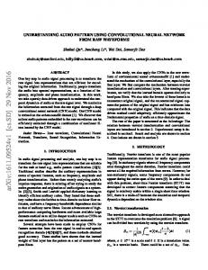
Fig. 1. The proposed FSRCNN networks achieve better super-resolution quality than existing methods, and are tens of times faster. Especially, the FSRCNN-s can run in real-time (> 24 fps) on a generic CPU. The chart is based on the Set14 [9] results summarized in Tables 3 and 4.

original LR image). For the upscaling factor n, the computational cost of convolution with the interpolated LR image will be n2 times of that for the original LR one. This is also the restriction for most learning-based SR methods [10,3,4,5,7,8]. If the network was learned directly from the original LR image, the acceleration would be significant, i.e., about n2 times faster. The second restriction lies on the costly non-linear mapping step. In SRCNN, input image patches are projected on a high-dimensional LR feature space, then followed by a complex mapping to another high-dimensional HR feature space. Dong et al. [2] show that the mapping accuracy can be substantially improved by adopting a wider mapping layer, but at the cost of the running time. For example, the large SRCNN (SRCNNEx) [2] has 57,184 parameters, which are six times larger than that for SRCNN (8,032 parameters). Then the question is how to shrink the network scale while still keeping the previous accuracy. According to the above observations, we investigate a more concise and efficient network structure for fast and accurate image SR. To solve the first problem, we adopt a deconvolution layer to replace the bicubic interpolation. To further ease the computational burden, we place the deconvolution layer1 at the end of the network, then the computational complexity is only proportional to the spatial size of the original LR image. It is worth noting that the deconvolution layer is not equal to a simple substitute of the conventional interpolation kernel like in FCN [13], or ‘unpooling+convolution’ like [14]. Instead, it consists of diverse automatically learned upsampling kernels (see Figure 3) that work jointly to generate the final HR output, and replacing these deconvolution filters with uniform interpolation kernels will result in a drastic PSNR drop (e.g., at least 0.9 dB on the Set5 dataset [15] for ×3). For the second problem, we add a shrinking and an expanding layer at the beginning and the end of the mapping layer separately to restrict mapping in a low-dimensional feature space. Furthermore, we decompose a single wide mapping layer into several layers with a fixed filter size 3 × 3. The overall shape of the new structure looks like an 1

We follow [11] to adopt the terminology ‘deconvolution’. We note that it carries very different meaning in classic image processing, see [12].

Accelerating the Super-Resolution Convolutional Neural Network

3

hourglass, which is symmetrical on the whole, thick at the ends and thin in the middle. Experiments show that the proposed model, named as Fast Super-Resolution Convolutional Neural Networks (FSRCNN) 2 , achieves a speed-up of more than 40× with even superior performance than the SRCNN-Ex. In this work, we also present a small FSRCNN network (FSRCNN-s) that achieves similar restoration quality as SRCNN, but is 17.36 times faster and can run in real time (24 fps) with a generic CPU. As shown in Figure 1, the FSRCNN networks are much faster than contemporary SR models yet achieving superior performance. Apart from the notable improvement in speed, the FSRCNN also has another appealing property that could facilitate fast training and testing across different upscaling factors. Specifically, in FSRCNN, all convolution layers (except the deconvolution layer) can be shared by networks of different upscaling factors. During training, with a well-trained network, we only need to fine-tune the deconvolution layer for another upscaling factor with almost no loss of mapping accuracy. During testing, we only need to do convolution operations once, and upsample an image to different scales using the corresponding deconvolution layer. Our contributions are three-fold: 1) We formulate a compact hourglass-shape CNN structure for fast image super-resolution. With the collaboration of a set of deconvolution filters, the network can learn an end-to-end mapping between the original LR and HR images with no pre-processing. 2) The proposed model achieves a speed up of at least 40× than the SRCNN-Ex [2] while still keeping its exceptional performance. One of its small-size version can run in real-time (>24 fps) on a generic CPU with better restoration quality than SRCNN [1]. 3) We transfer the convolution layers of the proposed networks for fast training and testing across different upscaling factors, with no loss of restoration quality.

2

Related Work

Deep learning for SR: Recently, the deep learning techniques have been successfully applied on SR. The pioneer work is termed as the Super-Resolution Convolutional Neural Network (SRCNN) proposed by Dong et al. [1,2]. Motivated by SRCNN, some problems such as face hallucination [16] and depth map super-resolution [17] have achieved state-of-the-art results. Deeper structures have also been explored in [18] and [19]. Different from the conventional learning-based methods, SRCNN directly learns an end-to-end mapping between LR and HR images, leading to a fast and accurate inference. The inherent relationship between SRCNN and the sparse-codingbased methods ensures its good performance. Based on the same assumption, Wang et al. [8] further replace the mapping layer by a set of sparse coding sub-networks and propose a sparse coding based network (SCN). With the domain expertise of the conventional sparse-coding-based method, it outperforms SRCNN with a smaller model size. However, as it strictly mimics the sparse-coding solver, it is very hard to shrink the sparse coding sub-network with no loss of mapping accuracy. Furthermore, all these 2

The implementation is available on the project page http://mmlab.ie.cuhk.edu.hk/ projects/FSRCNN.html.

4

Chao Dong et al.

networks [8,18,19] need to process the bicubic-upscaled LR images. The proposed FSRCNN does not only perform on the original LR image, but also contains a simpler but more efficient mapping layer. Furthermore, the previous methods have to train a totally different network for a specific upscaling factor, while the FSRCNN only requires a different deconvolution layer. This also provides us a faster way to upscale an image to several different sizes. CNNs acceleration: A number of studies have investigated the acceleration of CNN. Denton et al. [20] first investigate the redundancy within the CNNs designed for object detection. Then Zhang et al. [21] make attempts to accelerate very deep CNNs for image classfication. They also take the non-linear units into account and reduce the accumulated error by asymmetric reconstruction. Our model also aims at accelerating CNNs but in a different manner. First, they focus on approximating the existing well-trained models, while we reformulate the previous model and achieves better performance. Second, the above methods are all designed for high-level vision problems (e.g., image classification and object detection), while ours are for the low-level vision task. As the deep models for SR contain no fully-connected layers, the approximation of convolution filters will severely impact the performance.

3

Fast Super-Resolution by CNN

We first briefly describe the network structure of SRCNN [1,2], and then we detail how we reformulate the network layer by layer. The differences between FSRCNN and SRCNN are presented at the end of this section. 3.1

SRCNN

SRCNN aims at learning an end-to-end mapping function F between the bicubicinterpolated LR image Y and the HR image X. The network contains all convolution layers, thus the size of the output is the same as that of the input image. As depicted in Figure 2, the overall structure consists of three parts that are analogous to the main steps of the sparse-coding-based methods [10]. The patch extraction and representation part refers to the first layer, which extracts patches from the input and represents each patch as a high-dimensional feature vector. The non-linear mapping part refers to the middle layer, which maps the feature vectors non-linearly to another set of feature vectors, or namely HR features. Then the last reconstruction part aggregates these features to form the final output image. The computation complexity of the network can be calculated as follows, O{(f12 n1 + n1 f22 n2 + n2 f32 )SHR },

(1)

where {fi }3i=1 and {ni }3i=1 are the filter size and filter number of the three layers, respectively. SHR is the size of the HR image. We observe that the complexity is proportional to the size of the HR image, and the middle layer contributes most to the network parameters. In the next section, we present the FSRCNN by giving special attention to these two facets.

Accelerating the Super-Resolution Convolutional Neural Network

SRCNN

5

Bicubic interpolation

Original low-resolution image Patch extraction and representation

Non-linear Mapping

Reconstruction

High-resolution image

No pre-processing

FSRCNN Feature extraction

Shrinking

Mapping

Expanding

Deconvolution

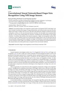
Fig. 2. This figure shows the network structures of the SRCNN and FSRCNN. The proposed FSRCNN is different from SRCNN mainly in three aspects. First, FSRCNN adopts the original low-resolution image as input without bicubic interpolation. A deconvolution layer is introduced at the end of the network to perform upsampling. Second, The non-linear mapping step in SRCNN is replaced by three steps in FSRCNN, namely the shrinking, mapping, and expanding step. Third, FSRCNN adopts smaller filter sizes and a deeper network structure. These improvements provide FSRCNN with better performance but lower computational cost than SRCNN.

3.2

FSRCNN

As shown in Figure 2, FSRCNN can be decomposed into five parts – feature extraction, shrinking, mapping, expanding and deconvolution. The first four parts are convolution layers, while the last one is a deconvolution layer. For better understanding, we denote a convolution layer as Conv(fi , ni , ci ), and a deconvolution layer as DeConv(fi , ni , ci ), where the variables fi , ni , ci represent the filter size, the number of filters and the number of channels, respectively. As the whole network contains tens of variables (i.e., {fi , ni , ci }6i=1 ), it is impossible for us to investigate each of them. Thus we assign a reasonable value to the insensitive variables in advance, and leave the sensitive variables unset. We call a variable sensitive when a slight change of the variable could significantly influence the performance. These sensitive variables always represent some important influential factors in SR, which will be shown in the following descriptions. Feature extraction: This part is similar to the first part of SRCNN, but different on the input image. FSRCNN performs feature extraction on the original LR image without interpolation. To distinguish from SRCNN, we denote the small LR input as Ys . By doing convolution with the first set of filters, each patch of the input (1-pixel overlapping) is represented as a high-dimensional feature vector. We refer to SRCNN on the choice of parameters – f1 , n1 , c1 . In SRCNN, the filter size of the first layer is set to be 9. Note that these filters are performed on the upscaled image Y . As most pixels in Y are interpolated from Ys , a 5 × 5 patch in Ys could cover almost all information of a 9 × 9 patch in Y . Therefore, we can adopt a smaller filter size f1 = 5 with little information loss. For the number of channels, we follow SRCNN to set c1 = 1. Then we only need to determine the filter number n1 . From another

6

Chao Dong et al.

perspective, n1 can be regarded as the number of LR feature dimension, denoted as d – the first sensitive variable. Finally, the first layer can be represented as Conv(5, d, 1). Shrinking: In SRCNN, the mapping step generally follows the feature extraction step, then the high-dimensional LR features are mapped directly to the HR feature space. However, as the LR feature dimension d is usually very large, the computation complexity of the mapping step is pretty high. This phenomenon is also observed in some deep models for high-level vision tasks. Authors in [22] apply 1 × 1 layers to save the computational cost. With the same consideration, we add a shrinking layer after the feature extraction layer to reduce the LR feature dimension d. We fix the filter size to be f2 = 1, then the filters perform like a linear combination within the LR features. By adopting a smaller filter number n2 = s 24 fps) on almost all the test images. Moreover, the FSRCNN still outperforms the previous methods on the PSNR values especially for ×2 and ×3. We also notice that the FSRCNN achieves slightly lower PSNR than SCN on factor 4. This is mainly because that the SCN adopts two models of ×2 to upsample an image by ×4. We have also tried this strategy and achieved comparable results. However, as we pay more attention to speed, we still present the results of a single network. Compare using different training sets (following the literature). To follow the literature, we also compare the best PSNR results that are reported in the corresponding paper, as shown in Table 4. We also add another two competitive methods – KK [28] and A+ [5] for comparison. Note that these results are obtained using different datasets, and our models are trained on the 91-image and General-100 datasets. From Table 4, we can see that the proposed FSRCNN still outperforms other methods on most upscaling factors and datasets. We have also done comprehensive comparisons in terms of SSIM and IFC [29] in Table 5 and 6, where we observe the same trend. The reconstructed images of FSRCNN (shown in Figure 7 and 8), more examples can be found on the project page) are sharper and clearer than other results. In another aspect, the restoration quality of small models (FSRCNN-s and SRCNN) is slightly worse than large models (SRCNN-Ex, SCN and FSRCNN). In Figure 7, we could observe some ”jaggies” or ringing effects in the results of FSRCNN-s and SRCNN.

5

Conclusion

While observing the limitations of current deep learning based SR models, we explore a more efficient network structure to achieve high running speed without the loss of restoration quality. We approach this goal by re-designing the SRCNN structure, and achieves a final acceleration of more than 40 times. Extensive experiments suggest that the proposed method yields satisfactory SR performance, while superior in terms of run time. The proposed model can be adapted for real-time video SR, and motivate fast deep models for other low-level vision tasks. Acknowledgment. This work is partially supported by SenseTime Group Limited.

14

Chao Dong et al.

Table 3. The results of PSNR (dB) and test time (sec) on three test datasets. All models are trained on the 91-image dataset. test upscaling Bicubic dataset factor PSNR Time Set5 2 33.66 Set14 2 30.23 BSD200 2 29.70 Set5 3 30.39 Set14 3 27.54 BSD200 3 27.26 Set5 4 28.42 Set14 4 26.00 BSD200 4 25.97 -

SRF [7] PSNR Time 36.84 2.1 32.46 3.9 31.57 3.1 32.73 1.7 29.21 2.5 28.40 2.0 30.35 1.5 27.41 2.1 26.85 1.7

SRCNN [1] PSNR Time 36.33 0.18 32.15 0.39 31.34 0.23 32.45 0.18 29.01 0.39 28.27 0.23 30.15 0.18 27.21 0.39 26.72 0.23

SRCNN-Ex [2] PSNR Time 36.67 1.3 32.35 2.8 31.53 1.7 32.83 1.3 29.26 2.8 28.47 1.7 30.45 1.3 27.44 2.8 26.88 1.7

SCN [8] PSNR Time 36.76 0.94 32.48 1.7 31.63 1.1 33.04 1.8 29.37 3.6 28.54 2.4 30.82 1.2 27.62 2.3 27.02 1.4

FSRCNN-s PSNR Time 36.53 0.024 32.22 0.061 31.44 0.033 32.55 0.010 29.08 0.023 28.32 0.013 30.04 0.0052 27.12 0.0099 26.73 0.0072

FSRCNN PSNR Time 36.94 0.068 32.54 0.16 31.73 0.098 33.06 0.027 29.37 0.061 28.55 0.035 30.55 0.015 27.50 0.029 26.92 0.019

Table 4. The results of PSNR (dB) on three test datasets. We present the best results reported in the corresponding paper. The proposed FSCNN and FSRCNN-s are trained on both 91-image and General-100 dataset. More comparisons with other methods on PSNR, SSIM and IFC [29] can be found in the supplementary file. test upscaling Bicubic dataset factor PSNR Set5 2 33.66 Set14 2 30.23 BSD200 2 29.70 Set5 3 30.39 Set14 3 27.54 BSD200 3 27.26 Set5 4 28.42 Set14 4 26.00 BSD200 4 25.97

KK [28] PSNR 36.20 32.11 31.30 32.28 28.94 28.19 30.03 27.14 26.68

A+ [5] PSNR 36.55 32.28 31.44 32.59 29.13 28.36 30.28 27.32 26.83

SRF [7] SRCNN [1] SRCNN-Ex [2] PSNR PSNR PSNR 36.89 36.34 36.66 32.52 32.18 32.45 31.66 31.38 31.63 32.72 32.39 32.75 29.23 29.00 29.30 28.45 28.28 28.48 30.35 30.09 30.49 27.41 27.20 27.50 26.89 26.73 26.92

SCN [8] FSRCNN-s FSRCNN PSNR PSNR PSNR 36.93 36.58 37.00 32.56 32.28 32.63 31.63 31.48 31.80 33.10 32.61 33.16 29.41 29.13 29.43 28.54 28.32 28.60 30.86 30.11 30.71 27.64 27.19 27.59 27.02 26.75 26.98

Originalx/xPSNR

Bicubicx/x31.68xdB

SRFx/x33.53xdB

SRCNNx/x33.39xdB

SRCNN-Exx/x33.67xdB

SCNx/x33.61xdB

FSRCNN-sx/x33.43xdB

FSRCNNx/x33.85xdB

Fig. 7. The “lenna” image from the Set14 dataset with an upscaling factor 3.

Accelerating the Super-Resolution Convolutional Neural Network

15

Table 5. The results of PSNR (dB), SSIM and IFC [29] on the Set5 [30], Set14 [9] and BSD200 [25] datasets. test upscaling Bicubic KK [28] ANR [4] A+ [4] SRF [7] dataset factor PSNR/SSIM/IFC PSNR/SSIM/IFC PSNR/SSIM/IFC PSNR/SSIM/IFC PSNR/SSIM/IFC Set5 2 33.66/0.9299/6.10 36.20/0.9511/6.87 35.83/0.9499/8.09 36.55/0.9544/8.48 36.87/0.9556/8.63 Set14 2 30.23/0.8687/6.09 32.11/0.9026/6.83 31.80/0.9004/7.81 32.28/0.9056/8.11 32.51/0.9074/8.22 BSD200 2 29.70/0.8625/5.70 31.30/0.9000/6.26 31.02/0.8968/7.27 31.44/0.9031/7.49 31.65/0.9053/7.60 Set5 3 30.39/0.9299/6.10 32.28/0.9033/4.14 31.92/0.8968/4.52 32.59/0.9088/4.84 32.71/0.9098/4.90 Set14 3 27.54/0.7736/3.41 28.94/0.8132/3.83 28.65/0.8093/4.23 29.13/0.8188/4.45 29.23/0.8206/4.49 BSD200 3 27.26/0.7638/3.19 28.19/0.8016/3.49 28.02/0.7981/3.91 28.36/0.8078/4.07 28.45/0.8095/4.11 Set5 4 28.42/0.8104/2.35 30.03/0.8541/2.81 29.69/0.8419/3.02 30.28/0.8603/3.26 30.35/0.8600/3.26 Set14 4 26.00/0.7019/2.23 27.14/0.7419/2.57 26.85/0.7353/2.78 27.32/0.7471/2.74 27.41/0.7497/2.94 BSD200 4 25.97/0.6949/2.04 26.68/0.7282/2.22 26.56/0.7253/2.51 26.83/0.7359/2.62 26.89/0.7368/2.62

Table 6. The results of PSNR (dB), SSIM and IFC [29] on the Set5 [30], Set14 [9] and BSD200 [25] datasets. test upscaling SRCNN [1] SRCNN-Ex [2] SCN [8] FSRCNN-s FSRCNN dataset factor PSNR/SSIM/IFC PSNR/SSIM/IFC PSNR/SSIM/IFC PSNR/SSIM/IFC PSNR/SSIM/IFC Set5 2 36.34/0.9521/7.54 36.66/0.9542/8.05 36.76/0.9545/7.32 36.58/0.9532/7.75 37.00/0.9558/8.06 Set14 2 32.18/0.9039/7.22 32.45/0.9067/7.76 32.48/0.9067/7.00 32.28/0.9052/7.47 32.63/0.9088/7.71 BSD200 2 31.38/0.9287/6.80 31.63/0.9044/7.26 31.63/0.9048/6.45 31.48/0.9027/7.01 31.80/0.9074/7.25 Set5 3 32.39/0.9033/4.25 32.75/0.9090/4.58 33.04/0.9136/4.37 32.54/0.9055/4.56 33.16/0.9140/4.88 Set14 3 29.00/0.8145/3.96 29.30/0.8215/4.26 29.37/0.8226/3.99 29.08/0.8167/4.24 29.43/0.8242/4.47 BSD200 3 28.28/0.8038/3.67 28.48/0.8102/3.92 28.54/0.8119/3.59 28.32/0.8058/3.96 28.60/0.8137/4.11 Set5 4 30.09/0.8530/2.86 30.49/0.8628/3.01 30.82/0.8728/3.07 30.11/0.8499/2.76 30.71/0.8657/3.01 Set14 4 27.20/0.7413/2.60 27.50/0.7513/2.74 27.62/0.7571/2.71 27.19/0.7423/2.55 27.59/0.7535/2.70 BSD200 4 26.73/0.7291/2.37 26.92/0.7376/2.46 27.02/0.7434/2.38 26.75/0.7312/2.32 26.98/0.7398/2.41

Original3/3PSNR

SRCNN-Ex3/327.953dB

Bicubic3/324.043dB

SRF3/327.963dB

SRCNN3/327.583dB

SCN3/328.573dB

FSRCNN-s3/327.733dB

FSRCNN3/328.683dB

Fig. 8. The “butterfly” image from the Set5 dataset with an upscaling factor 3.

16

Chao Dong et al.

References 1. Dong, C., Loy, C.C., He, K., Tang, X.: Learning a deep convolutional network for image super-resolution. In: ECCV. (2014) 184–199 2. Dong, C., Loy, C.C., He, K., Tang, X.: Image super-resolution using deep convolutional networks. TPAMI 38(2) (2015) 295–307 3. Yang, C.Y., Yang, M.H.: Fast direct super-resolution by simple functions. In: ICCV. (2013) 561–568 4. Timofte, R., De Smet, V., Van Gool, L.: Anchored neighborhood regression for fast examplebased super-resolution. In: ICCV. (2013) 1920–1927 5. Timofte, R., De Smet, V., Van Gool, L.: A+: Adjusted anchored neighborhood regression for fast super-resolution. In: ACCV, Springer (2014) 111–126 6. Cui, Z., Chang, H., Shan, S., Zhong, B., Chen, X.: Deep network cascade for image superresolution. In: ECCV. (2014) 49–64 7. Schulter, S., Leistner, C., Bischof, H.: Fast and accurate image upscaling with superresolution forests. In: CVPR. (2015) 3791–3799 8. Wang, Z., Liu, D., Yang, J., Han, W., Huang, T.: Deeply improved sparse coding for image super-resolution. ICCV (2015) 370–378 9. Zeyde, R., Elad, M., Protter, M.: On single image scale-up using sparse-representations. In: Curves and Surfaces. (2012) 711–730 10. Yang, J., Wright, J., Huang, T.S., Ma, Y.: Image super-resolution via sparse representation. TIP 19(11) (2010) 2861–2873 11. Zeiler, M.D., Fergus, R.: Visualizing and understanding convolutional networks. In: ECCV, Springer (2014) 818–833 12. Xu, L., Ren, J.S., Liu, C., Jia, J.: Deep convolutional neural network for image deconvolution. In: NIPS. (2014) 1790–1798 13. Long, J., Shelhamer, E., Darrell, T.: Fully convolutional networks for semantic segmentation. In: CVPR. (2015) 3431–3440 14. Dosovitskiy, A., Tobias Springenberg, J., Brox, T.: Learning to generate chairs with convolutional neural networks. In: CVPR. (2015) 1538–1546 15. Bevilacqua, M., Roumy, A., Guillemot, C., Morel, M.L.A.: Low-complexity single-image super-resolution based on nonnegative neighbor embedding. In: BMVC. (2012) 16. Zhu, S., Liu, S., Loy, C.C., Tang, X.: Deep cascaded bi-network for face hallucination. In: ECCV. (2016) 17. Hui, T.W., Loy, C.C., Tang, X.: Depth map super resolution by deep multi-scale guidance. In: ECCV. (2016) 18. Kim, J., Lee, J.K., Lee, K.M.: Accurate image super-resolution using very deep convolutional networks. CVPR (2016) 19. Kim, J., Lee, J.K., Lee, K.M.: Deeply-recursive convolutional network for image superresolution. CVPR (2016) 20. Denton, E.L., Zaremba, W., Bruna, J., LeCun, Y., Fergus, R.: Exploiting linear structure within convolutional networks for efficient evaluation. In: NIPS. (2014) 1269–1277 21. Zhang, X., Zou, J., He, K., Sun, J.: Accelerating very deep convolutional networks for classification and detection. TPAMI (2015) 22. Min Lin, Qiang Chen, S.Y.: Network in network. arXiv:1312.4400 (2014) 23. He, K., Zhang, X., Ren, S., Sun, J.: Delving deep into rectifiers: Surpassing human-level performance on imagenet classification. In: ICCV. (2015) 1026–1034 24. Yang, C.Y., Ma, C., Yang, M.H.: Single-image super-resolution: A benchmark. In: ECCV. (2014) 372–386

Accelerating the Super-Resolution Convolutional Neural Network

17

25. Martin, D., Fowlkes, C., Tal, D., Malik, J.: A database of human segmented natural images and its application to evaluating segmentation algorithms and measuring ecological statistics. In: ICCV. Volume 2. (2001) 416–423 26. Huang, J.B., Singh, A., Ahuja, N.: Single image super-resolution from transformed selfexemplars. In: CVPR. (2015) 5197–5206 27. Jia, Y., Shelhamer, E., Donahue, J., Karayev, S., Long, J., Girshick, R., Guadarrama, S., Darrell, T.: Caffe: Convolutional architecture for fast feature embedding. In: ACM MM. (2014) 675–678 28. Kim, K.I., Kwon, Y.: Single-image super-resolution using sparse regression and natural image prior. TPAMI 32(6) (2010) 1127–1133 29. Sheikh, H.R., Bovik, A.C., De Veciana, G.: An information fidelity criterion for image quality assessment using natural scene statistics. TIP 14(12) (2005) 2117–2128 30. Sheikh, H.R., Bovik, A.C., De Veciana, G.: An information fidelity criterion for image quality assessment using natural scene statistics. TIP 14(12) (2005) 2117–2128