search. In the case (i), piece-wise linear functions are constructed and in the ... method and algorithms that dynamically estimate the Lipschitz information for the.
Acceleration of univariate global optimization algorithms working with Lipschitz functions and Lipschitz first derivatives Daniela Lera∗ and Yaroslav D. Sergeyev† ‡
Abstract This paper deals with two kinds of the one-dimensional global optimization problems over a closed finite interval: (i) the objective function f (x) satisfies the Lipschitz condition with a constant L; (ii) the first derivative of f (x) satisfies the Lipschitz condition with a constant M . In the paper, six algorithms are presented for the case (i) and six algorithms for the case (ii). In both cases, auxiliary functions are constructed and adaptively improved during the search. In the case (i), piece-wise linear functions are constructed and in the case (ii) smooth piece-wise quadratic functions are used. The constants L and M either are taken as values known a priori or are dynamically estimated during the search. A recent technique that adaptively estimates the local Lipschitz constants over different zones of the search region is used to accelerate the search. A new technique called the local improvement is introduced in order to accelerate the search in both cases (i) and (ii). The algorithms are described in a unique framework, their properties are studied from a general viewpoint, and convergence conditions of the proposed algorithms are given. Numerical experiments executed on 120 test problems taken from the literature show quite a promising performance of the new accelerating techniques. Key Words. Global optimization, Lipschitz derivatives, balancing local and global information, acceleration.
∗
Dipartimento di Matematica e Informatica, Universit`a degli Studi di Cagliari, Cagliari, Italy. Corresponding author. He works at the following institutions: University of Calabria, Rende, Italy; N.I. Lobatchevsky State University, Nizhni Novgorod, Russia; and Institute of High Performance Computing and Networking of the National Research Council of Italy. ‡ The study was supported by the ministry of education and science of Russian Federation, project 14.B37.21.0878. †
1
1
Introduction
Let us consider the one-dimensional global optimization problem of finding a point x∗ belonging to a finite interval [a, b] and the value f ∗ = f (x∗ ) such that f ∗ = f (x∗ ) = min{f (x) : x ∈ [a, b]},
(1.1)
where either the objective function f (x) or its first derivative f ′ (x) satisfy the Lipschitz condition, i.e., either |f (x) − f (y)| ≤ L|x − y|, or
|f ′ (x) − f ′ (y)| ≤ M |x − y|,
x, y ∈ [a, b], x, y ∈ [a, b],
(1.2) (1.3)
with constants 0 < L < ∞, 0 < M < ∞. Problems of this kind are worthy of a great attention because of at least two reasons. First, there exists a large number of real-life applications where it is necessary to solve univariate global optimization problems stated in various ways (see, e.g., [2, 3, 4, 5, 8, 10, 16, 18, 23, 24, 26, 28, 29, 30, 31, 32, 35, 36]). This kind of problems is often encountered in scientific and engineering applications (see, e.g., [9, 14, 15, 21, 24, 30, 31, 33, 36]), and, in particular, in electrical engineering optimization problems (see, e.g., [5, 6, 17, 20, 27, 33]). On the other hand, it is important to study one-dimensional methods proposed to solve problems (1.1), (1.2) and (1.1), (1.3) because they can be successfully extended to the multi-dimensional case by numerous schemes (see, for example, one-point based, diagonal, simplicial, space-filling curves, and other popular approaches in [7, 12, 13, 19, 21, 30, 33]). In the literature, there exist several methods for solving the problems (1.1), (1.2) and (1.1), (1.3) (see, for example, [12, 13, 30, 33, 21], etc.). For solving the problem (1.1), (1.2) Piyavskii (see [23]) has proposed a popular method that requires an a priori overestimate of the Lipschitz constant L of the function f (x): in the course of its work, the algorithm constructs piece-wise linear support functions for f (x) over every subinterval [xi−1 , xi ], i = 2, ..., k, where the points x1 , ..., xk are points previously produced by the algorithm (see Fig. 1) at which the objective function f (x) has been evaluated, i.e., zi = f (xi ), i = 2, ..., k. In the present paper, to solve the problem (1.1), (1.2) we consider Piyavskii’s method and algorithms that dynamically estimate the Lipschitz information for the entire region [a, b] or for its subregions. This is done since the precise information about the value L Piyavskii’s method requires for its correct work is often hard to get in practice. Thus, we use two different procedures to obtain an information on the constant L: the first one estimates the global constant during the search (the word “global” means that the same estimate is used over the whole region [a, b]), and the second, called “local tuning technique” that adaptively estimates the local Lipschitz constants in different subintervals of the search region during the course of the optimization process. Then, in order to accelerate the search, we propose a new acceleration tool, called “local improvement”, that can be used together with all three ways described above 2
6
4
2
f(x) 0
z i−1 zi
−2
−4
−6
x
i−1
x
i
Figure 1: A piece-wise linear support function constructed by the method of Piyavskii after five evaluations of the objective function f (x) to obtain the Lipschitz information in the framework of the Lipschitz algorithms. The new approach forces the global optimization method to make a local improvement of the best approximation of the global minimum immediately after a new approximation better than the current one is found. The proposed local improvement technique is of a particular interest due to the following reasons. First, usually in the global optimization methods the local search phases are separated from the global ones. This means that it is necessary to introduce a rule that stops the global phase and starts the local one; then it stops the local phase and starts the global one. It can happen (see, e.g., [12, 13, 30, 33, 21], etc.), that the global search and the local one are realized by different algorithms and the global search is not able to use all evaluations of f (x) made during the local search losing so an important information about the objective function that has been already obtained. The local improvement technique introduced in this paper does not have this defect and allows the global search to use all the information obtained during the local phases. In addition, it can work without any usage of the derivatives and this is a valuable asset when one solves the problem (1.1), (1.2) because, clearly, Lipschitz functions can be non-differentiable. Let us consider now the problem (1.1), (1.3). For this case, using the fact that the first derivative f ′ (x) of the objective function satisfies the Lipschitz condition (1.3), Breiman and Cutler (see [1]) have suggested an approach that constructs at each iteration piece-wise quadratic non-differentiable support functions for the function f (x) over [a, b] using an a priori given overestimate of M from (1.3). Gergel (see [8]) 3
6
4
2
f(x)
z i−1
0
zi
−2
−4
−6
x i−1
xi
Figure 2: Breiman-Cutler-Gergel piece-wise quadratic non-differentiable support function constructed after five evaluations of the objective function f (x) has proposed independently a global optimization method that constructs similar auxiliary functions (see Fig. 2) and estimates M dynamically during the search. If we suppose that the the Lipschitz constant M from (1.3) is known, then (see [1, 8]), at an iteration k > 2, the support functions Φi (x) are constructed for every interval [xi−1 , xi ], i = 2, ..., k, (see Fig. 2) as follows: x ∈ [xi−1 , xi ],
Φi (x) = max{ϕi−1 (x), ϕi (x)}, where ′ ϕi−1 (x) = zi−1 + zi−1 (x − xi−1 ) −
ϕi (x) = zi − zi′ (xi − x) −
(1.4)
M (x − xi−1 )2 , 2
M (xi − x)2 , 2
and zi = f (xi ), zi′ = f ′ (xi ). It can be noticed that in spite of the fact that f (x) is smooth, the support functions Φi (x) are not smooth. This defect has been eliminated in [25] where there have been introduced three methods constructing smooth support functions that are closer to the objective function than non-smooth ones. In this paper, for solving the problem (1.1), (1.3) we describe six different algorithms where smooth support functions are used. As it was in the case of the problem (1.1), (1.2), the local tuning and the local improvement techniques are applied to accelerate the search. 4
The paper has the following structure: in Section 2 we describe algorithms for solving the problem (1.1), (1.2); in Section 3 we describe methods that use smooth support functions in order to solve the problem (1.1), (1.3). The convergence conditions to the global minimizers for the introduced methods are established in both Sections. In Section 4, numerical results are presented and discussed. Finally, Section 5 concludes the paper.
2
Six methods constructing piece-wise linear auxiliary functions for solving problems with the Lipschitz objective function
In this Section, we study the problem (1.1) with the objective function f (x) satisfying the Lipschitz condition (1.2). First, we present a general scheme describing in a compact form all the methods considered in this Section and then, by specifying STEP 2 and STEP 4 of the scheme, we introduce six different algorithms. In this Section, by the term trial we denote the evaluation of the function f (x) at a point x that is called the trial point. General Scheme (GS) describing algorithms working with piece-wise linear auxiliary functions. STEP 0. The first two trials are performed at the points x1 = a and x2 = b. The point xk+1 , k ≥ 2, of the current (k+1)-th iteration is chosen as follows. STEP 1. Renumber the trial points x1 , x2 , . . . , xk of the previous iterations by subscripts so that a = x1 < . . . < xk = b. (2.1) STEP 2. Compute in a certain way the values li being estimates of the Lipschitz constants of f (x) over the intervals [xi−1 , xi ], i = 2, ...k. The way to calculate the values li will be specified in each concrete algorithm described below. STEP 3. Calculate for each interval (xi−1 , xi ), i = 2, ...k, its characteristic Ri =
zi + zi−1 (xi − xi−1 ) − li , 2 2
(2.2)
where the values zi = f (xi ), i = 1, ..., k. STEP 4. Find an interval (xt−1 , xt ) where the next trial will be executed. The way to choose such an interval will be specified in each concrete algorithm described below. STEP 5. If |xt − xt−1 | > ε, 5
(2.3)
where ε > 0 is a given search accuracy, then execute the next trial at the point xk+1 =
xt + xt−1 zt−1 − zt + 2 2lt
(2.4)
and go to STEP 1. Otherwise, take as an estimate of the global minimum f ∗ from (1.1) the value fk∗ = min{zi : 1 ≤ i ≤ k}, and a point
x∗k = arg min{zi : 1 ≤ i ≤ k},
as an estimate of the global minimizer x∗ , after executing these operations STOP. Let us make some observations with regard to the scheme GS introduced above. During the course of the (k+1)th iteration a method following this scheme constructs an auxiliary piece-wise linear function C k (x) =
k ∪
ci (x)
i=2
where ci (x) = max{zi−1 − li (x − xi−1 ), zi + li (x − xi )},
x ∈ [xi−1 , xi ],
and the characteristic Ri from (2.2) represents the minimum of the auxiliary function ci (x) over the interval [xi−1 , xi ]. If the constants li are equal or larger than the Lipschitz constant L for all i = 2, ..., k, then it follows from (1.2) that the function C k (x) is a low-bounding function for f (x) over the interval [a, b], i.e., for every interval [xi−1 , xi ], i = 2, ..., k, we have f (x) ≥ ci (x),
x ∈ [xi−1 , xi ],
i = 2, ..., k.
Moreover, if li = L, we obtain the Piyavskii support functions (see Fig. 1). In order to obtain from the general scheme GS a concrete global optimization algorithm, it is necessary to define STEP 2 and STEP 4 of the scheme. This section proposes six specific algorithms executing this operation in different ways. In STEP 2, we can make three different choices of computing the constant li that lead to three different procedures that are called STEP 2.1, STEP 2.2, and STEP 2.3, respectively. The first way to define STEP 2 is the following. STEP 2.1. Set li = L,
i = 2, ..., k.
(2.5)
Here the exact value of the a priori given Lipschitz constant is used. Obviously, this rule gives us the Piyavskii algorithm. 6
If the constant L it is not available (this situation be can very often encountered in practice), it is necessary to look for an approximation of L during the course of the search. Thus, as the second way to define STEP 2 of the GS we use an adaptive estimate of the global Lipschitz constant (see [30, 33]), for each iteration k. More precisely we have: STEP 2.2. Set li = r max{ξ, H k },
i = 2, ..., k,
(2.6)
where ξ > 0 is a small number that takes into account our hypothesis that f (x) is not constant over the interval [a, b] and r > 1 is a reliability parameter. The value H k is calculated as follows H k = max{Hi : i = 2, ..., k, } with Hi =
|zi − zi−1 | , xi − xi−1
i = 2, ..., k.
(2.7)
(2.8)
In both cases, STEP 2.1 and STEP 2.2, at each iteration k all quantities li assume the same value over the whole search region [a, b]. However, both the a priori given exact constant L and its global estimate (2.6) can provide a poor information about the behavior of the objective function f (x) over every small subinterval [xi−1 , xi ] ⊂ [a, b]. In fact, when the local Lipschitz constant related to the interval [xi−1 , xi ] is significantly smaller than the global constant L, then the methods using only this global constant or its estimate (2.6) can work slowly over such an interval (see [24, 30, 33]). In order to overcome this difficulty, we consider a recent approach (see [24, 30, 33]) called the local tuning that adaptively estimates the values of the local Lipschitz constants related to the intervals [xi−1 , xi ], i = 2, ..., k (note that other techniques using different kinds of local information in global optimization can be found also in [21, 33, 34]). The auxiliary function C k (x) is then constructed by using these local estimates for each interval [xi−1 , xi ], i = 2, ..., k. This technique is described below as the rule STEP 2.3. STEP 2.3. Set li = r max{λi , γi , ξ}
(2.9)
λi = max{Hi−1 , Hi , Hi+1 }, i = 3, ..., k − 1,
(2.10)
with where Hi is from (2.8), and when i = 2 and i = k only H2 , H3 , and Hk−1 , Hk , should be considered, respectively. The value γi = H k
(xi − xi−1 ) , X max 7
(2.11)
where H k is from (2.7) and X max = max{xi − xi−1 : i = 2, ..., k}. The parameter ξ > 0 has the same sense as in STEP 2.2. Note that in (2.9) we consider two different components, λi and γi , that take into account respectively the local and the global information obtained during the previous iterations. When the interval [xi−1 , xi ] is large, the local information is not reliable and the global part γi has a decisive influence on li thanks to (2.9) and (2.11). When [xi−1 , xi ] is small, then the local information becomes relevant, γi is small (see (2.11)), and the local component λi assumes the key role. Thus, STEP 2.3 automatically balances the global and the local information available at the current iteration. It has been proved for a number of global optimization algorithms that the usage of the local tuning can accelerate the search significantly (see [24, 25, 26, 30, 31, 32, 33]). Let us introduce now possible ways to fix STEP 4 of the GS. At this step, we select an interval where a new trial will be executed. We consider both the traditional rule used, for example, in [23] and [33] and a new one that we shall call the local improvement technique. The traditional way to choose an interval for the next trial is the following. STEP 4.1. Select the interval (xt−1 , xt ) such that Rt = min{Ri : 2 ≤ i ≤ k}
(2.12)
and t is the minimal number satisfying (2.12). This rule used together with STEP 2.1 gives us Piyavskii’s algorithm. In this case, the new trial point xk+1 ∈ (xt−1 , xt ) is chosen in such a way that Rt = min{Ri : 2 ≤ i ≤ k} = ct (xk+1 ) = min{C k (x) : x ∈ [a, b]}. The new way to fix STEP 4 is introduced below. STEP 4.2 (the local improvement technique). f lag is a parameter initially equal to zero. imin is the index corresponding to the current estimate of the minimal value of the function, that is: zimin = f (ximin ) ≤ f (xi ), i = 1, ..., k. z k is the result of the last trial corresponding to a point xj in the line (2.1), i.e., xk = xj . IF (flag=1) THEN IF z k < zimin THEN imin = j. Local improvement: Alternate the choice of the interval (xt−1 , xt ) among t = imin+1 and t = imin, if imin = 2, ..., k−1, (if imin = 1 or imin = k take t = 2 or t = k, respectively) in such a way that for δ > 0 it follows |xt − xt−1 | > δ. 8
(2.13)
ELSE (flag=0) t = argmin{Ri : 2 ≤ i ≤ k} ENDIF flag=NOTFLAG(flag) The motivation of the introduction of STEP 4.2 presented above is the following. In STEP 4.1, at each iteration, we continue the search at an interval corresponding to the minimal value of the characteristic Ri , i = 2, ..., k (see (2.12)). This choice admits occurrence of such a situation where the search goes on for a certain finite (but possibly high) number of iterations at subregions of the domain that are “distant” from the best found approximation to the global solution and only successively concentrates trials at the interval containing a global minimizer. However, very often it is of a crucial importance to be able to find a good approximation of the global minimum in the lowest number of iterations. Due to this reason, in STEP 4.2 we take into account the rule (2.12) used in STEP 4.1 and related to the minimal characteristic, but we alternate it with a new selection method that forces the algorithm to continue the search in the part of the domain close to the best value of the objective function found up to now. The parameter “flag” assuming values 0 or 1 allows us to alternate the two methods of the selection. More precisely, in STEP 4.2 we start by identifying the index imin corresponding to the current minimum among the found values of the objective function f (x), and then we select the interval (ximin , ximin+1 ) located on the right of the best current point, ximin , or the interval on the left of ximin , i.e., (ximin−1 , ximin ). STEP 4.2 keeps working alternatively on the right and on the left of the current best point ximin until a new trial point with value less than zimin is found. The search moves from the right to the left of the best found approximation trying to improve it. However, since we are not sure that the found best approximation ximin is really located in the neighborhood of a global minimizer x∗ , the local improvement is alternated in STEP 4.2 with the usual rule (2.12) providing so the global search of new subregions possibly containing the global solution x∗ . The parameter δ defines the width of the intervals that can be subdivided during the phase of the local improvement. Note that the trial points produced during the phases of the local improvement (obviously, there can be more than one phase in the course of the search) are used during the further iterations of the global search in the same way as the points produced during the global phases. Let us consider now possible combinations of the different choices of STEP 2 and STEP 4 allowing us to construct the following six algorithms. PKC: GS with STEP 2.1 and STEP 4.1 (Piyavskii’s method with the a priori Known Constant L). GE: GS with STEP 2.2 and STEP 4.1 (the method using the Global Estimate of the Lipschitz constant L).
9
LT: GS with STEP 2.3 and STEP 4.1 (the method executing the Local Tuning on the local Lipschitz constants). PKC LI: GS with STEP 2.1 and STEP 4.2 (Piyavskii’s method with the a priori Known Constant L enriched by the Local Improvement technique). GE LI: GS with STEP 2.2 and STEP 4.2 (the method using the Global Estimate of L enriched by the Local Improvement technique). LT LI: GS with STEP 2.3 and STEP 4.2 (the method executing the Local Tuning on the local Lipschitz constants enriched by the Local Improvement technique). Let us consider convergence properties of the introduced algorithms by studying an infinite trial sequence {xk } generated by an algorithm belonging to the general scheme GS for solving problem (1.1), (1.2). We remind that the algorithm P KC is Piyavskii’s method and its convergence properties have been studied in [23]. In order to start we need the following definition. Definition 2.1 Convergence to a point x′ ∈ (a, b) is said to be bilateral if there exist two infinite subsequences of {xk } converging to x′ one from the left, the other from the right. Theorem 2.1 Assume that the objective function f (x) satisfies the condition (1.2), and let x′ be any limit point of {xk } generated by the GE or by the LT algorithm. Then the following assertions hold: 1. convergence to x′ is bilateral, if x′ ∈ (a, b); 2. f (xk ) ≥ f (x′ ), for all trial points xk , k ≥ 1; 3. if there exists another limit point x′′ ̸= x′ , then f (x′′ ) = f (x′ ); 4. if the function f (x) has a finite number of local minima in [a, b], then the point x′ is locally optimal; 5. (Sufficient conditions for convergence to a global minimizer). Let x∗ be a global minimizer of f (x). If there exists an iteration number k ∗ such that for all k > k ∗ the inequality lj(k) ≥ Lj(k) (2.14) holds, where Lj(k) is the Lipschitz constant for the interval [xj(k)−1 , xj(k) ] containing x∗ , and lj(k) is its estimate (see (2.6) and (2.9)). Then the set of limit points of the sequence {xk } coincides with the set of global minimizers of the function f (x). Proof. The proofs of assertions 1–5 are analogous to the proofs of Theorems 4.1–4.2 and Corollaries 4.1–4.4 from [33]. 2 10
Theorem 2.2 Assertions 1–5 of Theorem 2.1 hold for the algorithms P KC LI, GE LI, and LT LI for a fixed finite tolerance δ > 0 and ε = 0, where δ is from (2.13) and ε is from (2.3). Proof. Since δ > 0 and ε = 0, the algorithms P KC LI, GE LI, and LT LI use the local improvement only at the initial stage of the search until the selected interval (xt−1 , xt ) is greater than δ. When |xt − xt−1 | ≤ δ the interval cannot be divided by the local improvement technique and the selection criterion (2.12) is used. Thus, since the one-dimensional search region has a finite length and δ is a fixed finite number, there exists a finite iteration number j such that at all iterations k > j only selection criterion (2.12) will be used. As a result, at the remaining part of the search, the methods P KC LI, GE LI, and LT LI behave themselves as the algorithms P KC, GE, and LT , respectively. This consideration concludes the proof. 2 The next theorem ensures existence of the values of the parameter r satisfying condition (2.14) providing so that all global minimizers of f (x) will be located by the four proposed methods that do not use the a priori known Lipschitz constant. Theorem 2.3 For any function f (x) satisfying (1.2) with L < ∞ there exists a value r∗ such that for all r > r∗ condition (2.14) holds for the four algorithms GE, LT , GE LI, and LT LI. Proof. It follows from (2.6), (2.9), and the finiteness of ξ > 0 that approximations of the Lipschitz constant li in the four methods are always greater than zero. Since L < ∞ in (1.2) and any positive value of the parameter r can be chosen in the scheme GS, it follows that there exists an r∗ such that condition (2.14) will be satisfied for all global minimizers for r > r∗ . This fact, due to Theorems 2.1 and 2.2, proves the theorem. 2
3
Six methods constructing smooth piece-wise quadratic auxiliary functions for solving problems with the Lipschitz first derivative
In this Section, we study the algorithms for solving problem (1.1) with the Lipschitz condition (1.3) that holds for the first derivative f ′ (x) of the objective function f (x). In this Section, by the term trial we denote the evaluation of both the function f (x) and its first derivative f ′ (x) at a point x that is called the trial point. We consider the smooth support functions described in [25]. This approach is based on the fact observed in [25], namely, that at each interval [xi−1 , xi ] (see Fig. 3) the curvature of the objective function f (x) is determined by the Lipschitz constant M from (1.3). In particular, over the interval (yi′ , yi ) it should be f (x) ≥ πi (x) where πi (x) = 0.5M x2 + bi x + ci . 11
(3.1)
6
4
πi(x) 2
f(x) φi−1
0
φi
−2
−4
−6
x i−1 y’ i
yi
xi
Figure 3: Constructing smooth support functions by using ϕi−1 (x), πi (x), and ϕi (x) This means that over the interval (yi′ , yi ) both the objective function f (x) and the parabola πi (x) are strictly above the Breiman-Cutler-Gergel’s function Φi (x) from (1.4) where the unknowns bi , ci , yi′ , and yi can be determined following the considerations made in [25]. These results from [25] allow us to construct the following smooth support function ψi (x) for f (x) over [xi−1 , xi ]: ′ ϕi−1 (x), x ∈ [xi−1 , yi ],
ψi (x) = πi (x), ϕi (x),
x ∈ [yi′ , yi ], x ∈ [yi , xi ]
(3.2)
where there exists the first derivative ψi′ (x), x ∈ [xi−1 , xi ], and ψi (x) ≤ f (x),
x ∈ [xi−1 , xi ].
This function is shown in Fig. 4. The points yi , yi′ and the vertex x¯i of the parabola πi (x) can be found (see [25] for the details) as follows: yi =
′ ′ xi−1 + 0.5M (x2i − x2i−1 ) zi−1 − zi + zi′ xi − zi−1 xi − xi−1 zi′ − zi−1 + + , (3.3) ′ 4 4M M (xi − xi−1 ) + zi′ − zi−1
yi′ = −
′ ′ xi−1 + 0.5M (x2i − x2i−1 ) zi−1 − zi + zi′ xi − zi−1 xi − xi−1 zi′ − zi−1 − + , (3.4) ′ 4 4M M (xi − xi−1 ) + zi′ − zi−1
12
6
4
2
f(x)
zi−1
0
zi
ψi(x)
−2
−4
−6
x i−1
xi
Figure 4: The resulting smooth support functions ψi (x) x¯i = 2yi −
1 ′ z − xi , M i
(3.5)
where zi = f (xi ) and zi′ = f ′ (xi ). In order to construct global optimization algorithms by applying the same methodology used in the previous Section, for each interval [xi−1 , xi ] we should calculate its characteristic Ri . For the smooth auxiliary functions ψi (x) it can be calculated as Ri = ψi (pi ), where pi = arg min{ψi (x) : x ∈ [xi−1 , xi ]}. Three different cases can take place. i) The first one is shown in Fig. 4. It corresponds to the situation where conditions ψi′ (yi′ ) < 0 and ψi′ (yi ) > 0 hold. In this case pi = arg min{f (xi−1 , ψi (¯ xi ), f (xi )} and Ri = min{f (xi−1 ), ψi (¯ xi ), f (xi )}.
(3.6)
ii) The second case is whenever ψi′ (yi′ ) ≥ 0 and ψi′ (yi ) > 0. In this situation, we have (see [25]) that Ri = min{f (xi−1 ), f (xi )}. (3.7) iii) The third case is when ψi′ (yi′ ) < 0 and ψi′ (yi ) ≤ 0. It can be considered by a complete analogy with the previous one. 13
We are ready now to introduce the general scheme for the methods working with smooth piece-wise quadratic auxiliary functions. As it has been done in the previous Section, six different algorithms will be then constructed by specifying STEP 2 and STEP 4 of the general scheme. General Scheme describing algorithms working with the first Derivatives and constructing smooth piece-wise quadratic auxiliary functions (GS D). STEP 0. The first two trials are performed at the points x1 = a and x2 = b. The point xk+1 , k ≥ 2, of the current (k+1)-th iteration is chosen as follows. STEP 1. Renumber the trial points x1 , x2 , . . . , xk of the previous iterations by subscripts so that a = x1 < . . . < xk = b. (3.8) STEP 2. Compute in a certain way the values mi being estimates of the Lipschitz constants of f ′ (x) over the intervals [xi−1 , xi ], i = 2, ...k. The way to calculate the values mi will be specified in each concrete algorithm described below. STEP 3. Initiate the index sets I = ∅, Y ′ = ∅, and Y = ∅. Set the index of the current interval i = 2 and go to STEP 3.1. STEP 3.1. If for the current interval [xi−1 , xi ] the following inequality πi′ (yi′ ) · πi′ (yi ) ≥ 0
(3.9)
does not hold (where π ′ (x) is the derivative of the parabola (3.1)) then go to STEP 3.2. Otherwise go to STEP 3.3. STEP 3.2. Calculate for the interval [xi−1 , xi ] its characteristic Ri using (3.6). Include i in I and go to STEP 3.4. STEP 3.3. Calculate for the interval [xi−1 , xi ] its characteristic Ri using (3.7). If f (xi−1 ) < f (xi ) then include the index i in the set Y ′ and go to STEP 3.4. Otherwise include i in the set Y and go to STEP 3.4. STEP 3.4. If i < k, set i = i + 1 and go to STEP 3.1. Otherwise go to STEP 4. STEP 4. Find the interval (xt−1 , xt ) for the next possible trial. The way to do it will be specified in each concrete algorithm described below. STEP 5. If |xt − xt−1 | > ε,
14
(3.10)
where ε > 0 is a given search accuracy, then execute the next trial at the point x
k+1
′ yt ,
= x¯t , yt ,
if t ∈ Y ′ , if t ∈ I, if t ∈ Y,
(3.11)
and go to STEP 1. Otherwise, take as an estimate of the global minimum f ∗ from (1.1) the value fk∗ = min{zi : 1 ≤ i ≤ k}, and a point
x∗k = arg min{zi : 1 ≤ i ≤ k},
as an estimate of the global minimizer x∗ , after executing these operations STOP. Let us make just two comments upon the introduced scheme GS D. First, in STEPS 3.1–3.4 the characteristics Ri , i = 2, ..., k, are calculated by taking into account the different cases i – iii of the location of the point pi described above. Second, note that the index sets I, Y , and Y ′ have been introduced in order to calculate the new trial point xk+1 in STEP 5. In fact, the vertex x¯i of the i − th parabola, i = 2, ..., k, can be outside the interior of the interval [xi−1 , xi ]. It can happen that x¯i ∈ / [xi−1 , xi ] whenever ψi′ (yi′ ) ≥ 0 and ψi′ (yi ) > 0 (or ψi′ (yi′ ) < 0 and ′ ψi (yi ) ≤ 0), and so the point yi′ (or yi ) is selected as new trial point xk+1 . Let us show now how it is possible to specify STEP 2 and STEP 4 of the scheme GS D. As it has been done in the previous Section for the scheme GS, we first describe three different choices of the values mi that should be done at STEP 2 and then consider two selection rules that can be used to fix STEP 4 for choosing the point xk+1 . The first possible way to assign values to mi is the following: STEP 2.1 Set mi = M,
i = 2, ..., k,
(3.12)
where M is from (1.3). In this case, the exact value of the a priori given Lipschitz constant for the first derivative f ′ (x) is used. As a result, the auxiliary functions ψi (x) from (3.2) are support functions for f (x) over the intervals [xi−1 , xi ], i = 2, ..., k. Since it is difficult to know the exact value M in practice, the choices made in the following STEPS 2.2 and 2.3 (as it was for the methods working with Lipschitz objective functions) describe how to estimate dynamically the global constant M (STEP 2.2) and the local constants related to each interval [xi−1 , xi ], i = 2, ..., k (STEP 2.3). STEP 2.2 Set mi = r max{ξ, H k }, 15
i = 2, ..., k,
(3.13)
where ξ > 0 reflects the supposition that f ′ (x) is not constant over the interval [a, b] and r > 1 has the same sense as in the STEP 2.2 of the scheme GS. The value H k is computed as H k = max{vi : i = 2, ..., k}, where vi =
′ |2(zi−1 − zi ) + (zi−1 + zi′ )(xi − xi−1 )| + di (xi − xi−1 )2
(3.14)
(3.15)
and √
di =
′ ′ |2(zi−1 − zi ) + (zi−1 + zi′ )(xi − xi−1 )|2 + (zi′ − zi−1 )2 (xi − xi−1 )2 .
(3.16)
If an algorithm uses the exact value M of the Lipschitz constant (see STEP 2.1 above) then it is ensured by construction that the points yi′ , yi from (3.4) and (3.3) belong to the interval [xi−1 , xi ]. In the case, when an estimate mi of M is used, it can happen that, if the value mi is underestimated, the points yi′ and yi can be obtained outside the interval [xi−1 , xi ] that would lead to an error in the work of the algorithm using such an underestimate. It has been proved in [25] that the choice (3.13)–(3.16) makes this unpleasant situation impossible. More precisely, the following theorem holds. Theorem 3.1 If the values mi in GS D are determined by formulae (3.13)-(3.16) then the points yi′ , yi from (3.3), (3.4) belong to the interval [xi−1 , xi ] and the following estimates take place: yi′ − xi−1 ≥
(r − 1)2 (xi − xi−1 ), 4r(r + 1)
(r − 1)2 xi − y i ≥ (xi − xi−1 ). 4r(r + 1) Let us introduce now STEP 2.3 that shows how the local tuning technique works in the situation where the first derivative of the objective function can be calculated. STEP 2.3 Set mi = r max{λi , γi , ξ},
(3.17)
where r > 1 and ξ > 0 have the same sense as before, and λi = max{vi−1 , vi , vi+1 }, i = 3, ..., k − 1,
(3.18)
where the values vi are calculated following (3.15), and when i = 2 and i = k we consider only v2 , v3 , and vk−1 , vk , respectively. The value γi is computed as follows (xi − xi−1 ) , (3.19) γi = H k X max 16
where H k is from (3.14) and X max = max{(xi − xi−1 ), 1 = 2, ..., k}. As it was in STEP 2.3 of the scheme GS from the previous Section, the local tuning technique balances the local and the global information to get the estimates mi on the basis of the local and the global estimates λi and γi . Note also that the fact that yi′ and yi belong to the interval [xi−1 , xi ] can be proved by a complete analogy with Theorem 3.1 above. Let us consider now STEP 4 of the scheme GS D. At this step, we should select an interval [xt−1 , xt ] containing the next trial point xk+1 . As we have already done in Section 2, we consider two strategies: the rule selecting the interval corresponding to the minimal characteristic Rt and the local improvement technique. Thus, STEP 4.1 and STEP 4.2 of the scheme GS D correspond exactly to STEP 4.1 and STEP 4.2 of the scheme GS from Section 2. The obvious difference consists of the fact that characteristics Ri , i = 2, ..., k are calculated with respect to STEPS 3.1–3.4 of the scheme GS D. Thus, by specifying STEP 2 and STEP 4 we obtain from the general scheme GS D the following six algorithms: DKC: GS D with STEP 2.1 and STEP 4.1 (the method using the first Derivatives and the a priori Known Lipschitz Constant M ). DGE: GS D with STEP 2.2 and STEP 4.1 (the method using the first Derivatives and the Global Estimate of the Lipschitz constant M ). DLT: GS D with STEP 2.3 and STEP 4.1 (the method using the first Derivatives and the Local Tuning). DKC LI: GS D with STEP 2.1 and STEP 4.2 (the method using the first Derivatives, the a priori Known Lipschitz Constant M , and the Local Improvement technique). DGE LI: GS D with STEP 2.2 and STEP 4.2 (the method using the first Derivatives, the Global Estimate of the Lipschitz constant M , and the Local Improvement technique). DLT LI: GS D with STEP 2.3 and STEP 4.2 (the method using the first Derivatives, the Local Tuning, and the Local Improvement technique). Let us consider now infinite trial sequences {xk } generated by methods belonging to the general scheme GS D and study convergence properties of the six algorithms introduced above.
17
Theorem 3.2 Assume that the objective function f (x) satisfies condition (1.3), and let x′ (x′ ̸= a, x′ ̸= b) be any limit point of {xk } generated by either by the method DKC or the DGE or the DLT . If the values mi , i = 2, ..., k, are bounded as below vi ≤ mi < ∞,
(3.20)
where vi is from (3.15), then the following assertions hold: 1. convergence to x′ is bilateral, if x′ ∈ (a, b); 2. f (xk ) ≥ f (x′ ), for all trial points xk , k ≥ 1; 3. if there exists another limit point x′′ ̸= x′ , then f (x′′ ) = f (x′ ); 4. if the function f (x) has a finite number of local minima in [a, b], then the point x′ is locally optimal; 5. (Sufficient conditions for convergence to a global minimizer). Let x∗ be a global minimizer of f (x) and [xj(k)−1 , xj(k) ] be an interval containing this point during the course of the k-th iteration of one of the algorithms DKC, DGE, or DLT . If there exists an iteration number k ∗ such that for all k > k ∗ the inequality Mj(k) ≤ mj(k) < ∞
(3.21)
takes places for [xj(k)−1 , xj(k) ] and (3.20) for all the other intervals, then the set of limit points of the sequence {xk } coincides with the set of global minimizers of the function f (x). Proof. The proofs of assertions 1–5 are analogous to the proofs of Theorems 5.1–5.5 and Corollaries 5.1–5.6 from [25]. 2 The fulfillment of the sufficient conditions for convergence to a global minimizer, i.e., (3.21), are evident for the algorithm DKC. For the methods DGE and DLT , its fulfillment depends on the choice of the reliability parameter r. A theorem similar to the theorem 2.3 can be proved for them by a complete analogy. However, there exist particular cases where the objective function f (x) is such that its structure ensures that (3.21) holds. In the following theorem, sufficient conditions providing the fulfillment of (3.21) for the methods DGE and DLT are established for a particular class of objective functions. The theorem states that if f (x) is quadratic in a neighborhood I(x∗ ) of the global minimizer x∗ , then to ensure the global convergence it is sufficient that the methods will place one trial point on the left from x∗ and one trial point on the right from x∗ . Theorem 3.3 If the objective function f (x) is such that there exists a neighborhood I(x∗ ) of a global minimizer x∗ where f (x) = 0.5M x2 + qx + n,
(3.22)
where q and n are finite constants and M is from (1.3) and trials have been executed at points x− , x+ ∈ I(x∗ ), then condition (3.21) holds for algorithms DGE and DLT and x∗ is a limit point of the trial sequences generated by these methods if (3.20) is fulfilled for all the other intervals. 18
Proof. The proof is analogous to the proof of Theorem 5.6 from [25].
2
Theorem 3.4 Assertions 1–5 of Theorem 3.2 hold for the algorithms DKC LI, DGE LI, and DLT LI for a fixed finite tolerance δ > 0 and ε = 0, where δ is from (2.13) and ε is from (2.3). Proof. The proof is analogous to the proof of Theorem 2.2 from Section 2.
4
2
Numerical experiments
In this section, we present numerical results executed on 120 functions taken from the literature to compare the performance of the six algorithms described in Section 2 and the six algorithms from Section 3. Two series of experiments have been done. In both of them the choice of the reliability parameter r has been done with the step 0.1 starting from r = 1.1, i.e., r = 1.1, 1.2, etc. in order to ensure convergence to the global solution for all the functions taken into consideration in each series. It is well known (see detailed discussions on the choice of r and its influence on the speed of Lipschitz global optimization methods in [21, 30, 33]) that in general, for higher values of r methods of this kind are more reliable but slower. It can be seen from the results of experiments (see Tables 1 – 6) that the tested methods were able to find the global solution already for very low values of r. Then, since there is no sense to make a local improvement with the accuracy δ that is higher than the final required accuracy ε, in all the algorithms using the local improvement technique the accuracy δ from (2.13) has been fixed δ = ε. Finally, the technical parameter ξ (used only when at the initial iterations a method executes trials at the points with equal values) has been fixed to ξ = 10−8 for all the methods using it. In the first series of experiments, a set of 20 functions described in [11] has been considered. In Tables 1 and 2, we present numerical results for the six methods proposed to work with the problem (1.1), (1.2). In particular, Table 1 contains the numbers of trials executed by the algorithms with the accuracy ε = 10−4 (b − a), where ε is from (2.3). Table 2 presents the results for ε = 10−6 (b−a). The parameter r = 1.1 was sufficient for the algorithms GE, LT , and GE LI, LT LI while the exact values of the Lipschitz constant of the functions f (x) have been used in the methods P KC and P KC LI. In Tables 3 and 4, we present numerical results for the six methods proposed to work with the problem (1.1), (1.3). We have considered the same two accuracies in Tables 1 and 2: ε = 10−4 (b − a) for the experiments shown in Table 3 and ε = 10−6 (b − a) for the results presented in Table 4. The reliability parameter r has been taken equal to 1.2. All the global minima have been found by all the methods in all the experiments presented in Tables 1–4. In the last rows of Tables 1 – 4, the average values of the numbers of trials points generated by the algorithms are given. The first (quite obvious) observation that can be made with respect to the performed experiments 19
Problem 1 2 3 4 5 6 7 8 9 10 11 12 13 14 15 16 17 18 19 20 Average
PKC 149 155 195 413 151 129 153 185 119 203 373 327 993 145 629 497 549 303 131 493 314.60
GE 158 127 203 322 142 90 140 184 132 180 428 99 536 108 550 588 422 257 117 70 242.40
LT 37 36 145 45 46 84 41 126 44 43 74 71 73 43 62 79 100 44 39 70 65.10
PKC LI 37 33 67 39 151 39 41 55 37 43 47 45 993 39 41 41 43 41 39 41 95.60
GE LI 35 35 25 39 145 41 33 41 37 37 43 33 536 25 37 43 79 39 31 37 68.55
LT LI 35 35 41 37 53 41 35 29 35 39 37 35 75 27 37 41 81 37 33 33 40.80
Table 1: Results of numerical experiments executed on 20 test problems from [11] by the six methods belonging to the scheme GS; the accuracy ε = 10−4 (b − a), r = 1.1 consists of the fact that the methods using derivatives are faster than the methods that do not use this information (compare results in Tables 1 and 2 with the results in Tables 3 and 4, respectively). Then, it can be seen from Tables 1 and 2 that both accelerating techniques, the local tuning and the local improvement, allow us to speed up the search significantly when we work with the methods belonging to the scheme GS. With respect to the local tuning we can see that the method LT is faster than the algorithms P KC and GE. Analogously, the LT LI is faster than the methods P KC LI and GE LI. The introduction of the local improvement also was very successful. In fact, the algorithms P KC LI, GE LI, and LT LI work significantly faster than the methods P KC, GE, and LT , respectively. The effect of the local tuning and local improvement techniques is very well marked in the case of the problem (1.1), (1.2), i.e., when the first derivative of the objective function is not available. In the case of methods proposed to solve the problem (1.1), (1.3), where the derivative of the objective function can be used to construct algorithms, the effect of the introduction of the two acceleration techniques is always present but is not so strong (see Tables 3 and 4). This happens because the smooth auxiliary functions constructed by all the methods belonging to the scheme GS D are much better than the piece-wise linear functions build by the methods belonging to the class GS. The smooth auxiliary functions are very close to the objective function f (x) providing so already in the case of the slowest DKC 20
Problem 1 2 3 4 5 6 7 8 9 10 11 12 13 14 15 16 17 18 19 20 Average
PKC 1681 1285 1515 4711 1065 1129 1599 1641 1315 1625 4105 3351 8057 1023 7115 4003 5877 3389 1417 2483 2919.30
GE 1242 1439 1496 3708 1028 761 1362 1444 1386 1384 3438 1167 6146 1045 4961 6894 4466 2085 1329 654 2371.75
LT 60 58 213 66 67 81 64 194 64 65 122 114 116 66 103 129 143 67 60 66 95.90
PKC LI 55 53 89 63 59 63 65 81 61 59 71 67 8057 57 65 63 69 65 61 61 464.20
GE LI 55 61 51 63 65 65 55 67 59 63 63 57 6146 49 61 65 103 61 57 61 366.35
LT LI 57 57 61 59 74 61 59 49 57 57 61 55 119 49 59 63 103 57 53 53 63.15
Table 2: Results of numerical experiments executed on 20 test problems from [11] by the six methods belonging to the scheme GS; the accuracy ε = 10−6 (b − a), r = 1.1 algorithm a very good speed and, as a result, leaving less space for a possible acceleration that can be obtained thanks to applying the local tuning and/or the local improvement techniques. However, also in this case, the algorithm DLT LI is two times faster than the method DKC (see Tables 3 and 4). Finally, it can be clearly seen from Tables 1 – 4 that the acceleration effects produced by both techniques are more pronounced when the accuracy of the search increases. This effect takes place for the methods belonging to both schemes, GS and GS D. In the second series of experiments, a class of 100 one-dimensional randomized test functions from [22] has been taken. Each function fj (x), j = 1, ..., 100, of this class is defined over the interval [−5, 5] and has the following form fj (x) = 0.025(x − x∗j )2 + sin2 ((x − x∗j ) + (x − x∗j )2 ) + sin2 (x − x∗j ),
(4.1)
where the global minimizer x∗j , j = 1, ..., 100, is chosen randomly from interval [−5, 5] and differently for the 100 functions of the class. Fig. 5 shows the graph of the function no. 38 from the set of test functions (4.1) and the trial points generated by the 12 methods while minimizing this function, with accuracy ε = 10−4 (b − a). The global minimum of the function, f ∗ = 0, is attained at the point x∗ = 3.3611804993. In Fig. 5 the effects of the acceleration techniques, the local tuning and the local improvement, can be clearly seen. Table 5 shows the average numbers of trial points generated by the six methods that do not use the derivative of the objective functions, while Table 6 contains the 21
Problem 1 2 3 4 5 6 7 8 9 10 11 12 13 14 15 16 17 18 19 20 Average
DKC 15 10 48 14 17 22 10 44 10 9 24 19 197 13 55 66 51 5 11 22 33.10
DGE 16 12 58 14 16 24 12 52 13 12 26 21 63 17 43 54 45 9 11 24 27.10
DLT 14 12 56 11 15 22 11 50 12 12 22 21 25 17 17 26 32 9 11 25 21.00
DKC LI 15 10 57 14 17 21 11 45 10 9 26 19 37 14 43 49 33 5 11 19 23.25
DGE LI 16 13 27 14 20 25 13 25 13 12 25 23 45 20 33 45 39 9 11 23 22.55
DLT LI 15 13 25 11 18 21 11 25 13 12 21 21 26 20 18 26 27 9 11 25 18.40
Table 3: Results of numerical experiments executed on 20 test problems from [11] by the six methods belonging to the scheme GS D; the accuracy ε = 10−4 (b − a), r = 1.2 results of the six methods that use the derivative. In columns 2 and 4, the values of the reliability parameter r are given. In Table 5, the asterisk denotes that in the algorithm LT LI (for ε = 10−4 (b − a)) the value r=1.3 has been used for 99 functions, and for the function no. 32 the value r=1.4 has been applied. Tables 5 and 6 confirm for the second series of experiments the same conclusions that have been made with respect to the effects of the introduction of the acceleration techniques for the first series of numerical tests.
5
Conclusions
In this paper, there have been considered two kinds of the one-dimensional global optimization problems over a closed finite interval: (i) problems where the objective function f (x) satisfies the Lipschitz condition with a constant L; (ii) problems where the first derivative of f (x) satisfies the Lipschitz condition with a constant M . Two general schemes describing numerical methods for solving both problems have been described. Six particular algorithms have been presented for the case (i) and six algorithms for the case (ii). In both cases, auxiliary functions constructed and adaptively improved during the search have been used. In the case (i), piecewise linear functions have been described and constructed. In the case (ii), smooth piece-wise quadratic functions have been applied. 22
Problem 1 2 3 4 5 6 7 8 9 10 11 12 13 14 15 16 17 18 19 20 Average
DKC 22 12 57 19 21 26 12 48 12 11 37 27 308 16 87 101 73 5 13 24 46.55
DGE 22 16 69 19 19 27 16 61 16 16 37 31 93 21 66 81 66 14 15 27 36.60
DLT 16 16 66 16 18 26 15 60 15 16 29 28 29 21 21 28 38 14 15 27 25.70
DKC LI 22 12 63 19 21 27 13 49 12 11 37 29 55 17 67 65 51 5 13 25 30.65
DGE LI 22 17 37 20 24 28 18 33 16 17 35 31 61 25 51 63 61 14 15 28 30.80
DLT LI 17 17 35 17 22 28 16 33 16 17 29 27 30 25 22 28 39 14 15 28 23.75
Table 4: Results of numerical experiments executed on 20 test problems from [11] by the six methods belonging to the scheme GS D; the accuracy ε = 10−6 (b − a), r = 1.2 In the introduced methods, the Lipschitz constants L and M for the objective function and its first derivative were either taken as values known a priori or were dynamically estimated during the search. A recent technique that adaptively estimates the local Lipschitz constants over different zones of the search region was used to accelerate the search in both cases (i) and (ii) together with a newly introduced technique called the local improvement. Convergent conditions of the described twelve algorithms have been studied. The proposed local improvement technique is of a particular interest due to the following reasons. First, usually in the global optimization methods the local search phases are separated from the global ones. This means that it is necessary to introduce a rule that stops the global phase and starts the local one; then it stops the local phase and starts the global one. It happens very often that the global search and the local one are realized by different algorithms and the global search is not able to use all evaluations of the objective function made during the local search losing so an important information about the objective function that has been already obtained. The local improvement technique introduced in this paper does not have this drawback and allows the global search to use all the information obtained during the local phases. In addition, it can work both with and without the derivatives and this is a valuable asset when one solves the Lipschitz global optimization problems 23
4
2
0 PKC
421
GE
163
LT
43
PKC−LI
41
GE−LI
37
LT−LI
33
DKC
132
DGE
78
DLT
26
DKC−LI
35
DGE−LI
31
DLT−LI
19
−5
−4
−3
−2
−1
0
1
2
3
4
5
Figure 5: Graph of the function number 38 from (4.1) and trial points generated by the 12 methods while minimizing this function. because, clearly, Lipschitz functions can be non-differentiable. Numerical experiments executed on 120 test problems taken from the literature have shown quite a promising performance of the new accelerating techniques.
References [1] L. Breiman and A. Cutler. A deterministic algorithm for global optimization. Mathematical Programming, 58(1–3):179–199, 1993. [2] J. M. Calvin. An adaptive univariate global optimization algorithm and its convergence rate under the Wiener measure. Informatica, 22(4):471–488, 2011.
24
Method PKC GE LT PKC LI GE LI LT LI
r
1.1 1.1 1.1 1.3*
ε = 10−4 400.54 167.63 47.28 44.82 40.22 38.88
r
1.1 1.1 1.2 1.2
ε = 10−6 2928.48 1562.27 70.21 65.70 62.96 60.04
Table 5: Average number of trial points generated by the six methods belonging to the scheme GS on 100 test functions from [22] with the accuracies ε = 10−4 and ε = 10−6 Method DKC DGE DLT DKC LI DGE LI DLT LI
r
1.1 1.1 1.1 1.1
ε = 10−4 125.85 87.53 49.00 43.72 38.46 28.50
r
1.1 1.1 1.1 1.1
ε = 10−6 170.65 121.01 53.53 62.88 58.61 40.57
Table 6: Average number of trial points generated by the six methods belonging to the scheme GS D on 100 test functions from [22] with the accuracies ε = 10−4 and ε = 10−6 ˘ One-dimensional global optimization for ob[3] J. M. Calvin and A. Zilinskas. servations with noise. Computers and Mathematics with Applications, 50(1– 2):157–169, 2005. [4] L. G. Casado, I. Garcia, and Ya. D. Sergeyev. Interval algorithms for finding the minimal root in a set of multiextremal non-differentiable one-dimensional functions. SIAM J. Scientific Computing, 24(2):359–376, 2002. [5] P. Daponte, D. Grimaldi, A. Molinaro, and Ya. D. Sergeyev. An algorithm for finding the zero-crossing of time signals with Lipschitzean derivatives. Measurement, 16(1):37–49, 1995. [6] P. Daponte, D. Grimaldi, A. Molinaro, and Ya. D. Sergeyev. Fast detection of the first zero-crossing in a measurement signal set. Measurement, 19(1):29–39, 1996. [7] C. A. Floudas and P. M. Pardalos. State of the Art in Global Optimization. Kluwer Academic Publishers, Dordrecht, 1996. [8] V. P. Gergel. A global search algorithm using derivatives. In Yu.I. Neymark, editor, Systems Dynamics and Optimization, pages 161–178. N. Novgorod University Press, 1992.
25
[9] K. Hamacher. On stochastic global optimization of one-dimensional functions. Physica A: Statistical Mechanics and its Applications, 354(15 August 2005):547–557, 2005. [10] E. R. Hansen. Global optimization using interval analysis: The one-dimensional case. J. Optim. Theory Appl., 29(3):251–293, 1979. [11] P. Hansen, B. Jaumard, and H. Lu. Global optimization of univariate lipschitz functions: 1-2. Mathematical Programming, 55:251–293, 1992. [12] R. Horst and P. M. Pardalos, editors. Handbook of Global Optimization, volume 1. Kluwer Academic Publishers, Dordrecht, 1995. [13] R. Horst and H. Tuy. Global Optimization – Deterministic Approaches. Springer–Verlag, Berlin, 1996. [14] D. E. Johnson. Introduction to Filter Theory. Prentice Hall Inc., New Jersey, 1976. [15] D. Kalra and A. H. Barr. Guaranteed ray intersections with implicit surface. Computer Graphics, 23(3):297–306, 1989. [16] D. E. Kvasov and Ya. D. Sergeyev. A univariate global search working with a set of Lipschitz constants for the first derivative. Optimization Letters, 3(2):303– 318, 2009. [17] H. Y.-F. Lam. Analog and Digital Filters-Design and Realization. Prentice Hall Inc., New Jersey, 1979. [18] M. Locatelli. Bayesian algorithms for one-dimensional global optimization. J. Global Optimization, 10(1):57–76, 2001. [19] R. Mladineo. Convergence rates of a global optimization algorithm. Mathematical Programming, 54:223–232, 1992. [20] A. Molinaro and Ya. D. Sergeyev. Finding the minimal root of an equation with the multiextremal and nondifferentiable left-hand part. Numerical Algorithms, 28(1–4):255–272, 2001. [21] J. D. Pint´er. Global Optimization in Action (Continuous and Lipschitz Optimization: Algorithms, Implementations and Applications). Kluwer Academic Publishers, Dordrecht, 1996. [22] J. D. Pint´er. Global optimization: software, test problems, and applications. In P. M. Pardalos and H. E. Romeijn, editors, Handbook of Global Optimization, volume 2, pages 515–569. Kluwer Academic Publishers, Dordrecht, 2002. [23] S. A. Piyavskii. An algorithm for finding the absolute extremum of a function. Com. Maths. Math. Phys., 12:57–67, 1972. 26
[24] Ya. D. Sergeyev. A one-dimensional deterministic global minimization algorithm. Comput. Math. Math. Phys., 35(5):705–717, 1995. [25] Ya. D. Sergeyev. Global one-dimensional optimization using smooth auxiliary functions. Mathematical Programming, 81(1):127–146, 1998. [26] Ya. D. Sergeyev. Univariate global optimization with multiextremal nondifferentiable constraints without penalty functions. Computational Optimization and Applications, 34(2):229–248, 2006. [27] Ya. D. Sergeyev, P. Daponte, D. Grimaldi, and A. Molinaro. Two methods for solving optimization problems arising in electronic measurements and electrical engineering. SIAM J. Optim., 10(1):1–21, 1999. [28] Ya. D. Sergeyev, D. Famularo, and P. Pugliese. Index branch-and-bound algorithm for lipschitz univariate global optimization with multiextremal constraints. J. Global Optimization, 21(3):317–341, 2001. [29] Ya. D. Sergeyev and V.A. Grishagin. A parallel algorithm for finding the global minimum of univariate functions. J. Optimization Theory and Applications, 80(3):513–536, 1994. [30] Ya. D. Sergeyev and D. E. Kvasov. Diagonal Global Optimization Methods. FizMatLit, Moscow, 2008. In Russian. [31] Ya. D. Sergeyev, D. E. Kvasov, and F. M. H. Khalaf. A one-dimensional local tuning algorithm for solving GO problems with partially defined constraints. Optimization Letters, 1(1):85–99, 1995. [32] Ya. D. Sergeyev and D. L. Markin. An algorithm for solving global optimization problems with nonlinear constraints. J. Global Optim., 7(4):407–419, 1995. [33] R. G. Strongin and Ya. D. Sergeyev. Global optimization with non-convex constraints: Sequential and parallel algorithms. Kluwer Academic Publishers, Dordrecht, 2000. ˇ [34] A. T¨orn and A. Zilinskas. Global Optimization, volume 350 of Lecture Notes in Computer Science. Springer–Verlag, Berlin, 1989. ˘ [35] A. Zilinskas. Optimization of one-dimensional multimodal functions: Algorithm AS 133. Applied Statistics, 23:367–375, 1978. [36] M. A. Wolfe. On first zero crossing points. Applied Mathematics and Computation, 150:467–479, 2004.
27