Journal of Applied Psychology 2001, Vol. 86, No. 1, 114^121
Copyright 2001 by the American Psychological Association, Inc. 0021-9010/01/$5.00 DOI: 10.1037//0021-9010.86.1.114
Accounting for Common Method Variance in Cross-Sectional Research Designs Michael K. Lindell
David J. Whitney California State University, Long Beach
Texas A&M University
Cross-sectional studies of attitude-behavior relationships are vulnerable to the inflation of correlations by common method variance (CMV). Here, a model is presented that allows partial correlation analysis to adjust the observed correlations for CMV contamination and determine if conclusions about the statistical and practical significance of a predictor have been influenced by the presence of CMV. This method also suggests procedures for designing questionnaires to increase the precision of this adjustment.
Many theories used in applied psychology are based on the premise that behavior is a function of individuals' attitudes, beliefs, or perceptions of the situations in which they find themselves. For practical reasons, tests of theories such as Vroom's (1964) valence-instrumentality-expectancy theory and Fishbein and Ajzen's (1975) theory of reasoned action often have crosssectional rather than longitudinal designs. This means that individuals' reports of their internal states are collected at the same time as their reports of their past behavior related to those internal states. Consequently, the possibility arises that method variance (MV) has inflated the observed correlations between these two types of variables artifactually. Indeed, Feldman and Lynch (1988) have argued that the behavioral self-reports could be significantly correlated with job dimensions that are completely meaningless to the respondents if they are asked «o report their behavior and then provide ratings of job characteristics related to that behavior. More recent studies suggest that the MV problem is not this severe but does require further study (Crampton & Wagner, 1994; Harrison, McLaughlin, & Coalter, 1996). Many researchers have contended that MV problems can be solved by using multiple methods of measurement, and some have advocated analysis of multitrait-multimethod (MTMM) matrices by means of confirmatory factor analysis (Millsap, 1990; Mitchell, 1985; Podsakoff & Organ, 1986; Williams, Cote, & Buckley, 1989). However, MTMM matrix designs require at least twice as many measures as a conventional design. This forces the researcher either to limit the scope of a study (i.e., the number of constructs to be measured) or to accept a reduced response rate
when some members of a sample refuse to complete a lengthy questionnaire. To avoid these unappealing alternatives, some researchers have sought procedures that allow the effect of a method factor to be partialed out. Podsakoff and Todor (1985) argued that a pervasive method factor would manifest itself in a factor analysis and that partialing out the first factor would remove MV. They recognized that this would be a conservative procedure because some construct variance would be partialed out along with MV, but Kemery and Dunlap (1986) showed that the negative bias in this procedure is so large that partialing out the first factor would produce virtually meaningless results. Podsakoff and Organ (1986) later agreed with Kemery and Dunlap (1986), stating that "under these circumstances, interpretation of the results becomes difficult, if not impossible" (p. 537) and recommending that the variance accounted for by the first factor be reported only as a last resort. A Method Variance Model A clearer understanding of the MV problem can be gained by using the factor analysis model to illustrate the differences among the independent error (IE), common method variance (CMV), and unrestricted method variance (UMV) models. Specifically, the factor analysis model asserts that R = R* + 0, where R is the observed matrix of correlations among the variables, R* (=AA') is the matrix of correlations among the variables reproduced from the factor loadings (A) and the intercorrelation among the factors ($), and ® is a matrix of error variances (Hayduk, 1988). Under the IE model, ® is assumed to be diagonal (i.e., all off-diagonal elements are fixed at zero). By contrast, the UMV model asserts only that ® is not diagonal in form. This model can be considered the most general model because it allows the error terms to be correlated but does not fix or constrain the intercorrelations among those error terms. The CMV model is less restrictive than the IE model but more restrictive than the UMV model because it asserts that the observed variables are contaminated by a single unmeasured factor that has an equal effect on all of them. The CMV model is illustrated graphically in Figure 1, which shows two underlying constructs, Xf and X%, each of which has a single indicator, Xl and
Michael K. Lindell, Hazard Reduction and Recovery Center, Texas A&M University; David J. Whitney, Department of Psychology, California State University, Long Beach. This work was supported by National Science Foundation Grant BCS 9796297. We wish to thank Larry James and Larry Williams for discussions that led to the development of this model; however, none of the conclusions expressed here necessarily reflect anyone's views but ours. Correspondence concerning this article should be addressed to Michael K. Lindell, Hazard Reduction and Recovery Center, Texas A&M University, College Station, Texas 77843-3137. Electronic mail may be sent to
[email protected]. 114
METHOD VARIANCE
Figure 1. Path model of causal variables measured with error confounded with a method variable.
X2, respectively. Both Xf and X* cause Y*, which also has a single indicator, Y. The CMV model assumes that M has a constant correlation, r (which may turn out to be zero but is not assumed a priori to be so), with all of the manifest variables. Thus, all the off-diagonal elements in 0 are constrained to be equal to r (cf. Kemery & Dunlap, 1986). The variable M in the CMV model can be interpreted as an unmeasured relevant cause (L. R. James, Mulaik, & Brett, 1982) that is common to all of the observed variables in the model. If M is removed from Figure 1, the CMV model reduces to the IE model. If each of the observed variables has a distinct method variable, Mt, and all of the Mts are allowed to be intercorrelated with each other, then the CMV model generalizes to the UMV model (cf. Williams & Brown, 1994). If the manifest variables are measured without error and the rules of path analysis (Heise, 1975) are applied to Figure 1, one obtains three equations of the form, r
iMrjM