Dec 20, 2014 - culated numerical values of the fractal dimensions is analyzed as a ..... [6] B. B. Mandelbrot, Fractals: Form, Chance, and Dimension (San Fran-.
Accuracy of the box-counting algorithm
arXiv:1412.6664v1 [physics.data-an] 20 Dec 2014
for noisy fractals A. Z. G´orskia, M. Str´oz˙ a,b, P. O´swi¸ecimkaa, J. Skrzatc a
H. Niewodnicza´ nski Inst. of Nucl. Physics, Polish Acad. of Sci., Radzikowskiego 152, Krak´ow, 31-342
b
AGH University of Science and Technology, Faculty of Physics and Applied Computer Sci., Krak´ow
c
Dept. of Anatomy, Collegium Medicum, Jagellonian Univ., Krak´ow
Abstract The box-counting (BC) algorithm is applied to calculate fractal dimensions of four fractal sets. The sets are contaminated with an additive noise with amplitude γ = 10−5 ÷ 10−1 . The accuracy of calculated numerical values of the fractal dimensions is analyzed as a function of γ for different sizes of the data sample (ntot ). In particular, it has been found that a tiny (10−5 ) addition of noise generates much larger (three orders of magnitude) error of the calculated fractal exponents. Natural saturation of the error for larger noise values prohibits the power-like scaling. Moreover, the noise effect cannot be cured by taking larger data samples. PACS: 05.45.Df
1
1
Introduction
In last decades computations of fractal dimensions (exponents) have become very popular. A search through the Web of Science reveals about 10, 000 journal articles with the term fractal dimension in title, keywords, or abstract [1]. The fractal structures have been found in a wide spectrum of problems, ranging from high energy physics [2] to cosmology [3] and from bio-medical sciences [4] to econophysics [5]. Although the concept of fractal exponents has been popularized long time ago [6, 7], the accuracy of obtained results is usually either not discussed or overestimated. Moreover, it has been found that in quite a few papers misleading numerical results and conclusions have been published (see e.g.: [4, 8, 9, 10]). In many cases, especially for the time series analysis, the fractal exponents are computed indirectly, from the Hurst exponents. However, a simple relation between the two exponents holds only in some special cases [11]. What is more important, the computational algorithms of fractal exponents have systematic errors much larger than the corresponding statistical errors. This is mainly due to the finitness of the data sample (of size denoted by ntot ). This problem is independent on the computational algorithm applied. For the box-counting (BC) algorithm, it has been shown that the error (roughly) scales according to the power law, ∼ 1/nαtot [12], for pure fractals, without noise. The aim of this paper is to perform an analysis of the fractal structures contaminated with an additive external noise and to estimate the accuracy of the BC algorithm in these cases. A similar analysis for the influence
2
of noise on the Hurst exponents, which were computed by the MF-DFA method, has been performed recently [13]. It should be stressed that the type of algorithm is not so important, as the accuracy depends more on the choice of a particular fractal set than on the type of the algorithm applied. Algorithms that work better with some classes of the fractal sets are not so efficient for other classes (see e.g. Ref. [14]). We generate the mathematical fractal sets of different size (ntot ), namely, the standard (1/3) Cantor set (CS), 1/2-Cantor set (in 1-dimensional embedding space), Sierpi´ nski triangle and Sierpi´ nski carpet (in 2-dimensional embedding space). The data set {xi } is contaminated by the external additive noise, ξi (|ξi | ≤ 1), with different amplitudes γ
xi → xi + γ ξi .
(1)
For γ = 0, no external noise is present. The values of γ that will be considered are in the range 10−5 ÷ 10−1 (four orders of magnitude). Also, the size of the data sample, ntot , has been varied in the range 26 ÷ 220 (about four orders of magnitude). The fractal exponent has been calculated using the BC algorithm, according to the standard formula [6] P log i pqi (N) 1 lim , d(q) = 1 − q N →∞ log N
(2)
where N denotes the number of divisions, pi (N) is the measure of the subset in the ith box for a given division N and the box size ǫ = 1/N. In practical calculations the numerical data sets are always finite. Hence, the scaling
3
range (the limit N → ∞) is chosen as the interval within which the log-log plot is closest to the linear function. In fact, the problems with choosing the proper scaling range are the main sources of the systematic error. Furthermore, for monofractal sets one has d(q) = d0 = const. All cases discussed here are monofractals and one can set q = 0. In the following section, the numerical results will be presented and discussed. The final section is devoted to summary and conclusions.
2
Accuracy analysis
For our analysis, the well-known fractals embedded in the one- and twodimensional embedding space are taken, for which the precise theoretical values of thefractal exponents (dth ) are well known. Approximate values of these exponents (d) are calculated with the BC algorithm, according to Eq. (2), and the corresponding error is determined as follows
∆d = |dth − d| .
(3)
These computation is repeated for different values of the noise amplitude γ and for different values of the sample size ntot . In effect, one can find a dependence of the error on the noise strength and the sample size. Because ∆d ≤ E, from Eq. (3), it is clear that the error ∆d has the following upper bound ∆d ≤ E − dth ,
4
(4)
[ error ]
0.1
0.01
(A)
[ error ]
0.1
0.01 (B)
-5
10
-4
10
-3
10 [ noise amplitude ]
-2
10
-1
10
Figure 1: Error ∆d as a function of the noise amplitude (γ) for the standard Cantor set (A) and for the 1/2-Cantor set (B) with the different sizes of the data sample, ntot = 26 , 28 , 210 , 212 , 214 , 216 . The errors are denoted by the triangle-up, triangle-down, diamond, circle, star and cross symbols, respectively. In the last cases, the power-like fits are also added (solid lines). 5
where E is the embedding dimension. Hence, the error can be at most of order of 1. The question remains, how fast the bound (4) is reached. This will be studied below. First, the standard Cantor set and the 1/2-Cantor set were analyzed. The noise dependence of the errors was shown in Figs. 1-A and 1-B, respectively. Here, the different sample sizes are represented by the triangles-up, trianglesdown, diamonds, circles, stars and crosses, respectively. For larger data sets, the power fits were included for a comparison. From Fig. 1, it is clear that there is no power-like scaling of the error ∆d as a function of the noise amplitude (γ), especially for smaller data samples (. 103 ). Also, the value of the error for γ = 0.01 (i.e., the relative noise as small as about 1%) is rather large, of order 0.1 and the relative value of the error is close to 20%. A surprisingly large error induced by a small additive noise was also found for the fractal stochastic point processes (FSPP). For 106 data points the fractal dimension was estimated within ±0.1 accuracy, i.e., with the error higher than 10% [15]. Hence, the noise effect on the computational error is enhanced by at least one order of magnitude. In Fig 2., the error value is shown versus the sample size (ntot ). The different noise amplitudes, γ = 10−1 , 10−2 , 10−3, 10−4 , 10−5 , 0, are denoted by the triangle-up, triangle-down, diamond, circle, star, and cross symbols. The power fits for the smallest-noise amplitudes were also given for comparison. For the both fractals, the error value is almost independent of the sample size — it is dominated by the noise amplitude. Hence, by increasing the sample size one cannot improve numerical results. The triangle and diamond symbols are arranged almost horizontally. For a quite moderate noise (already below 6
[ error ]
0.1
0.01
(A) 0.001
[ error ]
0.1
0.01
(B) 0.001 2
10
3
4
10
10
5
10
[ ntot ]
Figure 2: Error ∆d as a function of the sample size (ntot ) for the standard Cantor set (A) and for the 1/2-Cantor set (B) with the different noise amplitudes, γ = 10−1 , 10−2 , 10−3, 10−4 , 10−5 , 0. The errors are denoted by the triangle-up triangle-down, diamond, circle, star and cross symbols, respectively. In the last cases, the power-like fits are added (solid lines).
7
[ error ]
0.1
0.01 (A)
[ error ]
0.1
0.01 (B)
-5
10
-4
10
-3
10 [ noise amplitude ]
-2
10
-1
10
Figure 3: Error ∆d as a function of the noise amplitude (γ) for the Sierpi´ nski triangle (A) and for the Sierpi´ nski carpet (B) with the different sizes of the data sample, ntot = 210 , 212 , 214 , 216 , 218 , 220 . The errors are denoted by the triangle-up triangle-down, diamond, circle, star and cross symbols, respectively. In the last cases, the power-like fits are added (solid lines).
8
1%, γ = 0.01 ÷ 0.001 — triangles and diamonds), the error approaches the bound (4). Moreover, for a very small noise (γ = 10−5 ), the errors are up to three orders of magnitude bigger than the noise itself. It is interesting to check whether the 2-D fractals are also so sensitive to an external noise. To this end, a similar analysis was performed for the Sierpi´ nski triangle (Figs. 3A, 4A) and for the Sierpi´ nski carpet (Figs. 3B, 4B). The fractal sets embedded in more dimensions are computationally more demanding. It have been estimated that in order to have a comparable accuracy for the fractals embedded in 2-D space, the number of data points should be squared, in comparison to the 1-D fractals [12]. Hence, the 2-D fractal sample sizes were taken in the range ntot = 210 ÷ 220 . In Fig. 3, the error dependence on the noise amplitude (γ) is shown for the Sierpi´ nski triangle (A) and for the Sierpi´ nski carpet (B). The different sample sizes, ntot = 210 , 212 , 214 , 216 , 218 , 220 , are represented by the triangle-up, triangle-down, diamond, circle, star and cross symbols, respectively. Again, an approximate power-like scaling is not observed. The total error (i.e. the sum of statistical and systematic errors, ∆d) was found in the range quite similar as for the 1-D fractals (Cantor sets). One can conclude that higher dimensional fractals are not more sensitive to an additive external noise than the 1-D fractals. However, the error remains considerably large, at least about 10% for a small (1% and less) noise and relatively large data samples (of order 105 ). The error (3) for a small noise (γ ≈ 10−5 ) is about three–four orders of magnitude larger (approaching 10−1 ). It is worth to mention that, in general, the external noise increases the calculated value of the fractal exponents. This is intuitively clear, as the 9
[ error ]
0.1
0.01 (A)
[ error ]
0.1
0.01 (B) 3
10
4
5
10
10
6
10
[ ntot ]
Figure 4: Error ∆d as a function of the sample size (ntot ) for the Sierpi´ nski triangle (A) and for the Sierpi´ nski carpet (B) with the different noise amplitudes, γ = 10−1 , 10−2 , 10−3, 10−4 , 10−5 , 0. The errors are denoted by the triangle-up triangle-down, diamond, circle, star and cross symbols, respectively. In last two cases, the power-like fits are added (solid lines).
10
white noise embedded in the E-dimensional space has the BC dimension equal to E. Hence, the obtained exponents for noisy fractals are usually overestimated and for large enough values of γ one gets results close to E. This effect prohibits the power-like scaling of ∆d as a function of γ. In addition, one reaches natural cut-off for larger noise values, ∆d ≤ E, where E is the embedding dimension of the fractal.
3
Summary and conclusions
In this paper the influence of an external additive noise with the amplitude γ on the BC-algorithm calculations of the fractal exponents, for the fractal sets of size ntot , was analysed. The numerical results are shown in Figs. 1–4. It has been found that the noise effect is surprisingly large — a relativly tiny external noise (γ = 10−5 ) implies the error values (3) up to three– four orders of magnitude larger. A small noise is usually a part of any real data under investigation. Hence, one should be very careful when drawing conclusions from numerically calculated fractal exponents for experimental data. As the error value is trivially limited by Eq. (4), for large noise amplitudes, the noise enhancement effect is saturated and a power-like scaling of this effect does not exist. A strong sensitivity to the noise is in agreement with the results obtained earlier for FSPP [15]. It is intuitively clear that the noise increases the computed fractal exponents, with the upper boumd ∆d ≤ E. Moreover, as can be seen from Figs. 2 and 4, the noise effect cannot be cured by taking much larger data samples. Already for the noise level 11
approaching 0.1%, the sample size becomes irrelevant. In conclusion, one should treat very carefully the numerical results of fractal exponents calculations for the data sets containing noise. This is very important since a small addition of noise is usually present in a majority of practical applications.
References [1] T. Gneiting, M. Schlather, SIAM Review 46, 269 (2003) [2] A. G´orski, Acta Phys. Pol. B15, 465 (1984); A. Bialas, R. Peszanski, Nucl. Phys. B 308, 803 (1988) [3] T. Chmaj, W. Doroba, W. Slomi´ nski, Z. Phys. C50, 333 (1991) [4] A. Z. G´orski, J. Skrzat, J. Anat. 208, 353 (2006) [5] A.Z. G´orski, S. Dro˙zd˙z, J. Speth, Physica A316, 496 (2002) [6] B. B. Mandelbrot, Fractals: Form, Chance, and Dimension (San Francisco: Freeman 1977) [7] J. Theiler, J. Opt. Soc. Am. A7, 1055 (1990) [8] A. Z. G´orski, J. Phys. A34, 7933 (2001) [9] J. L. McCauley, Physica A309, 183 (2002) [10] P. Castiglioni, Comput. Biol. Med. 40, 950 (2010) [11] S. Jaffard, SIAM J. Math. Anal. 28 944; 971, (1997) 12
[12] A. Z. G´orski, S. Dro˙zd˙z, A. Mokrzycka, J. Pawlik, Acta Phys. Pol. A121, B-28 (2012) [13] J. Ludescher, M. I. Bagachev, J. W. Kentelhardt, A. Y. Schumann, A. Bunde Physica A390, 2480 (2011) [14] J. Brewer, L. Di Girolamo, Atmospheric Res. 82, 433 (2006) [15] S. B. Lowen, M. C. Teich, Fractals 3, 183 (1995)
13