and water flows, was selected since it is based on soil properties that can be ..... bBC indicates analytic form proposed by Brooks and Corey [1964], and P ...
WATER RESOURCES RESEARCH, VOL. 44, W03432, doi:10.1029/2006WR005765, 2008
Accuracy of top soil moisture simulation using a mechanistic model with limited soil characterization A. Chanzy,1 M. Mumen,1 and G. Richard2 Received 23 November 2006; revised 10 December 2007; accepted 21 January 2008; published 29 March 2008.
[1] For many applications, soil water flow models require knowledge of soil properties
and conditions that is difficult to obtain. In this study, we analyzed the impact of approximations on model prediction of soil water content when only limited soil property data are available. The TEC model of Chanzy and Bruckler (1993), representing soil heat and water flows, was selected since it is based on soil properties that can be estimated with the pedotransfer function, and it is driven by standard climatic data. The impact of the choices made for soil hydraulic properties, initial soil water conditions, and lower boundary conditions for a wide range of soil were studied. In this study, emphasis was placed on estimating moisture in the surface soil layer (0–30 cm) and was limited to wet and moderately dry soil conditions, which can be critical for applications in agriculture to determine trafficable days and in surface hydrology. The results from this study indicate the importance of soil hydraulic properties and moisture profile initialization, which may lead to errors larger than 0.10 m3 m 3 on soil moisture in the surface layer. The pedotransfer function proposed by Wo¨sten (1997) led to the best simulated soil moisture in the top 30 cm, but initialization has a strong impact. Thus a ‘‘warming up’’ period of 70 days is needed to mitigate the initialization error. This duration can be reduced according to the amount of precipitation. We propose starting simulations 48 hours after the last significant rainfall with an initial water potential of 10 kPa. At the bottom of the soil, a gravitational flux at a depth of at least 80 cm is recommended to compute the boundary conditions. These recommendations for implementing a soil water transfer model were evaluated against independent experimental data, and a moisture accuracy (root mean square error) of 0.04 m3 m 3 was obtained. Citation: Chanzy, A., M. Mumen, and G. Richard (2008), Accuracy of top soil moisture simulation using a mechanistic model with limited soil characterization, Water Resour. Res., 44, W03432, doi:10.1029/2006WR005765.
1. Introduction [2] Soil water flow models require knowledge of soil properties and conditions that are highly variable in space and in time and time consuming and/or expensive to measure. For many applications that depend on soil moisture status, such as decision making for farming operations (e.g., irrigation, tillage) and implementing distributed hydrological models, measuring all the inputs of soil water transfer models remains unrealistic. In a sensitivity analysis, Mumen [2006] showed that in the case of bare soil, the most critical soil characteristics for estimating soil moisture with a soil water flow model are (1) soil hydraulic properties, i.e., water retention and hydraulic conductivity curves; (2) initial soil water status, i.e., change in water content or water potential with depth at the beginning of the simulation period; and (3) boundary conditions, i.e., climatic condi-
1 Unite´ Mixte de Recherche Environnement Me´diterrane´en et Mode´lisation des Agro-Hydrosyste`mes, Institut National de la Recherche Agronomique, Universite´ d’Avignon et des Pays de Vaucluse, Avignon, France. 2 Unite´ de Science du Sol d’Orle´ans, Institut National de la Recherche Agronomique, Ardon, France.
Copyright 2008 by the American Geophysical Union. 0043-1397/08/2006WR005765
tions at the soil surface and change in water content or water potential with depth. [3] Because of the difficulty and expense of measuring soil hydraulic and physical properties, numerous pedotransfer functions (PTFs) have been developed. They allow determining more difficult to measure soil properties than those which are easier to obtain (e.g., soil texture), and assessing their precision is still a topic of research [Kvaerno et al., 2007; Manyame et al., 2007; Stenitzer et al., 2007; Zeleke and Si, 2007]. The evaluation of soil hydraulic properties by using PTFs has been based either on soil property measurements or on a functional assessment that considers their impact on the outputs of soil water transfer models, e.g., the change in water content of a given layer, water flux of drainage at the soil bottom. Several studies aimed at evaluating PTFs using direct measurements of soil water retention and hydraulic conductivity curves have been performed with data from a great number of soils. The PTFs developed by Rawls and Brackensiek [1985], Vereecken et al. [1989], Vereecken et al. [1990], and Wo¨sten [1997] are often cited as yielding the best results when compared with soil properties measurements [Williams et al., 1992; Tietje and Tapkenhinrichs, 1993; Kern, 1995; Tietje and Hennings, 1996; Cornelis et al., 2001; Wagner et al., 2001]. In these studies, PTF evaluation was performed on a single soil
W03432
1 of 16
W03432
CHANZY ET AL.: ACCURACY OF TOP SOIL MOISTURE SIMULATION
hydraulic function (retention curve or hydraulic conductivity) considering four to 10 PTFs. When comparing PTFs, those of Wosten and Vereecken were found to be among the best in every case. In addition, the study carried out by Wagner et al. [2004] considered two hydraulic functions and again highlighted the interest of these PTFs. [4] On the contrary, the functional assessment of PTFs did not lead to any clear indication as to how to select a PTF. It appears that most of the studies were performed on a single soil type and with different evaluation criteria [Vereecken et al., 1992; Espino et al., 1996; Hack-ten Broeke and Hegmans, 1996; Christiaens and Feyen, 2001; Van Alphen et al., 2001; Minasny and McBratney, 2002; Starks et al., 2003; Mumen, 2006; Sonneveld et al., 2003]. More precisely, (1) Espino et al. [1996] concluded that implementing the SWATRE model with Vereecken’s PTFs led to biased soil moisture with an overestimation that sometimes exceeded 0.1 m3 m 3; (2) similar results were obtained by Sonneveld et al. [2003] with Wosten’s PTFs; (3) Christiaens and Feyen [2001] took Rawls’ and Brackensiek’s PTFs to run the MIKE SHE model and found a Coefficient of Variation higher than 20% for the average soil water content in grid cells. Encouraging results with better accuracy were given by Hack-ten Broeke and Hegmans [1996], Van Alphen et al. [2001], and Starks et al. [2003]. The study of Starks et al. [2003] was the only one to cover a wide range of soils using Rawls and Brackensiek’s PTFs. They obtained an accuracy better than 0.02 m3 m 3 for the water content in the top 60 cm layer, whereas errors near the surface were much higher (>0.05 m3 m 3 with certain soils). The sparse results found in the literature stress the need to perform a functional assessment of PTFs with a soilwater model. [5] The impact of initialization and lower boundary conditions have seldom been addressed. They were investigated by Vereecken et al. [1992], who found that the use of a free drainage or a fixed water potential as a lower boundary condition could induce changes in moisture supply capacity by 20%. However, we did not find general rules that set out clear strategies for initialization and/or lower boundary conditions. [6] The goals of this study were (1) to define options for implementing a soil water transfer model in a limited data context and (2) thus determine the accuracy expected for soil moisture. It was assumed that a limited data set includes commonly collected soil characteristics (texture, organic matter content) and standard climatic data. In order to focus only on soil functioning, the study was restricted to bare soil cases. Attention is also given to the plowed layer (0 – 30 cm depth) because of its importance in determining (1) trafficable days for agricultural operations and (2) water fluxes at the soil surface in the form of infiltration or runoff. As a consequence, the impact of the soil characteristics of deeper layers was minimized. Finally, the study is limited to periods having moderate evaporative demand (potential evaporation < 3 mm d 1) with various rainfall regimes (numerous light rainfalls, heavy rainfalls, and long drying periods). This choice, made primarily to address the question of trafficable days for agricultural operations, led us to consider wet and moderately dry soil conditions. The impact of soil properties (soil texture, soil structure) on soil moisture dynamics is the strongest in this range of moisture
W03432
conditions, and it is also that for which the most data are available. [7] In this study, a soil water transfer model was selected according to the following criteria. The model (1) had to be a physically based model to take advantage of the background available in the literature on the determination of soil hydraulic properties, (2) had to represent moisture vertical profiles, and (3) had to be driven by top boundary conditions inferred from standard climatic data. To fulfill the latter criterion, the water transfer model also had to represent the soil temperature profile to solve the energy balance at the soil surface, and then compute the evaporation flux without using empirical equations. The mechanistic model of soil heat and water flows (mode`le de Transferts Eau et Chaleur, or TEC model) from Chanzy and Bruckler [1993] was selected. A wide range of soil conditions were used to strengthen the generalization of the options proposed for running a soil transfer model. Finally, the proposed options were blind-tested on independent data sets.
2. Material and Method [8] All the simulations were done with the TEC model. A reference data set was established to analyze the different options chosen to overcome the lack of soil information. The proposed implementation options were then tested against a validation data set. 2.1. Soil Water Transfer Model [9] The TEC model is based on the heat and mass flow theory in partially saturated media [Philip and de Vries, 1957]. Water transport in liquid and vapor phases is considered and linked to the soil energy balance through vaporization and condensation. Partial differential equations, limited to vertical dimension, are solved by a Galerkin finite element method. Neumann (flux) or Dirichlet (state variable) boundary conditions can be implemented at the surface and at the bottom of the soil system. Water and heat flows at the surface are computed by solving the energy balance and considering the rainfall intensity. However, surface boundary conditions are switched to Dirichlet conditions when a water charge appears. Soil can be divided into three layers defined by homogeneous soil properties. Every layer is divided into several elements separated by nodes where the soil water potential and the temperature are computed. Time steps, varying from 0.5 to 600 s, are automatically computed according to the magnitude of the change of the computed state variables or the occurrence of a rainfall. The TEC model inputs are given in Table 1. 2.2. Reference Data Set [10] A reference data set was needed to evaluate the different options developed in this study in order to implement the TEC model with limited information. The use of experimental measurements would have been adequate. However, to gather experimental data covering a wide range of soils, it would have been necessary to obtain data from different databases acquired in various places, under different climates, and by different teams using different measurement protocols. It would then have been difficult to isolate the impact of model implementation strategies (use of PTFs, initialization, bottom boundary conditions) from other sources of variations such as measurement errors and
2 of 16
W03432
CHANZY ET AL.: ACCURACY OF TOP SOIL MOISTURE SIMULATION
W03432
Table 1. Inputs and Outputs of the TEC Model Parameters and Variables
Remarks Soil Properties
Water retention curve [h(q)] Hydraulic conductivity [K(q)] Gaseous diffusion coefficient [D(q)] Apparent heat conductivity [l(q)] Heat capacity [C(q)] Dry bulk density [rd]
defined for every soil layer
Surface Properties Albedo [a(q)] Surface emissivity (e) Aerodynamical roughness length (z0) Initialization Soil water potential profile [h(z)] Soil temperature profile [T(z)]
defined at each node
Lower Boundary Conditions Soil temperature (Dirichlet) [Tzmax(t)] or heat flux (Neumann) [qhZmax(t)] Water potential (Dirichlet) [hzmax(t)] or water flux (Neumann) [qwZmax(t)] Top Boundary Conditions Surface heat flow (G) and evaporation computed using the surface energy balance equations (E) (Neumann) or water charge (Dirichlet), derived from standard climatic data Main Outputs Temperature profile [Tz(t)] Water potential profile [hz(t)] Net radiation [Rn] Sensible (H) and latent (LE) energy fluxes Soil heat flux at the soil surface [G]
heat and water fluxes in the soil can be derived from the main outputs and soil properties
climatic contexts. To avoid such problems, a numerical database using the TEC model was built to simulate the reference cases. Sets of parameters from several former studies in which the TEC model was calibrated were gathered and validated against field measurements. Consequently, it was possible to simulate soil moisture variations representative of real soils under the same climatic conditions. Six soil cases covering a wide range of soil texture (Table 2) were selected. The soil depth was 80 cm for all the simulations, and one to three soil layers were considered according to vertical heterogeneity (Table 2). To illustrate the variability in soil hydraulic properties, retention curves [h(q)] and the hydraulic conductivity [K(q)] relationships of the surface layer are shown in Figure 1. [11] Reference simulations were computed with two climatic sequences applied to all soils. The first climatic sequence was measured at Estre´e-Mons (northern France, 48.99°N, 2.99°E). It represents an oceanic climate with frequent light rainfalls and moderate evaporative demand, with an average potential evaporation of 1.3 mm d 1 during the period considered. The second climatic sequence was measured at Avignon (southern France, 43.9°N, 4.91°E) in autumn. It represents a Mediterranean climate with heavy rain and long periods of dryness. The average potential evaporation was 2.6 mm d 1 during the period considered. The lower boundary conditions were determined at a depth of 80 cm with a constant water potential ( 33.3 kPa). The depth and temperatures were obtained from measurements carried out in soils from Estre´e-Mons and Avignon (silt loam and silty clay loam, respectively) under the climatic sequences used for the simulations. Constant water potential
was assumed to be realistic, since soil moisture in deep layers often varies slowly with bare soils. [12] An example of the reference results is illustrated in Figure 2. Since TEC model initialization is a source of uncertainty, a warming-up period was defined, intended to compute a realistic soil water potential and a temperature profile at the beginning of the period used to evaluate the options for implementing the TEC model. 2.3. Options for TEC Model Implementation With Limited Observations [13] The impacts of soil hydraulic properties, and initial and lower boundary conditions estimations, were addressed separately. Thus, when a property was considered, the other TEC inputs were those of the reference simulation. The analysis consisted of performing simulations during the evaluation period (Figure 2). The TEC model was then initialized with the profiles computed from the reference simulations. 2.3.1. Hydraulic Properties [14] To estimate soil hydraulic properties using limited soil information, we selected four PTFs to estimate soil hydraulic properties (h(q) and K(q)) to run the TEC model. Those of Vereecken et al. [1989, 1990], Rawls and Brackensiek [1985], and Wo¨sten [1997], hereinafter referred to as VER, BRA, and WOS, respectively, were chosen as being among the best PTFs in the intercomparison studies mentioned in the introduction. These PTFs are all based on soil texture and dry bulk density. Additionally, the WOS and VER PTFs both account for organic matter content while WOS is the only PTF that considers surface and deep
3 of 16
CHANZY ET AL.: ACCURACY OF TOP SOIL MOISTURE SIMULATION
W03432
W03432
Table 2. Soil Characteristics for Reference and Validation Case Study Soil ID CO-SiL MO-SiL MX-SL AL-SiL PO-SiCL AL-SiCL ME-C SL-TILL SL-NOTILL SiCLAL102
Depth, cm 0 – 80 0 – 33 33 – 80 0 – 20 20 – 80 0 – 10 10 – 40 40 – 80 0 – 10 10 – 25 25 – 80 0 – 10 10 – 40 40 – 80 0 – 20 20 – 80 0 – 22 22 – 30 0–5 5 – 30 0 – 20
Texture silt loam silt loam
Clay %
Sand %
silty loam
10.50 14.50 25.20 16.50 20.80 17.00 17.00 17.00 27.20 27.20 27.20 38.90 39.70 48.10 62.60 60.50 19.7
38.80 5.20 3.00 59.50 46.20 34.30 29.20 29.20 11.00 11.00 11.00 5.30 4.60 2.00 11.60 11.50 7.7
silty loam
24
6.2
silty clay loam
37.5
5.5
sandy loam silt loam silt clay loam silt clay loam clay
Bulk Density, g cm 3 1.44 1.28 1.52 1.48 1.23 1.24 1.28 1.46 1.29 1.40 1.60 1.30 1.35 1.60 1.13 1.37 1.176 1.356 1.172 1.456 1.20
20 – 40
Organic Matter, % 1.00 2.10 0.90 1.18 0.87 1.50 1.50 1.00 2.40 2.40 1.00 2.50 2.50 1.00 2.32 2.29 0.94 0.5 1.09 0.5 2.2
h(q)a c
VG VGc VGc VG VG VG VG VG VGc VGc VG VGOd VGd VGd VGc VGc
K(q)b
Reference
P Pc BC BC BC BC BC BC P P P BCe BCe BCe BC BC
Chanzy and Bruckler [1993] Sillon et al. [2003] Findeling et al [2003] Olioso et al. [2002a] Chanzy and Bruckler [1993] Olioso et al. [2002a] Aboudrare [2000] Mumen [2006] Mumen [2006] Olioso et al. [2002a]
1.43
a
VG indicates analytic form proposed by van Genuchten [1980]. BC indicates analytic form proposed by Brooks and Corey [1964], and P indicates polynomial model applied to log(K). c Indicates that several relationships were fitted to match the measurements. d VG function was modified in the dry region according to the Ross et al. [1991] approach. e A log linear function was applied near saturation [Olioso et al., 2002a]. b
layers separately. The PTF formulated by Cosby et al. [1984] was also considered since it requires the least soil information (texture only). All the PTFs selected were designed to estimate coefficients of the analytical functions representing h(q) and K(q). 2.3.2. Initialization [15] The problem of model initialization was addressed by choosing a starting time for the evaluation period considered favorable for making assumptions about soil moisture conditions. After being saturated, soils drain quickly thanks to water flows in macropores. It is generally accepted that soil dries until field capacity (soil moisture at approximately -33 kPa) within 1 or 2 days. Advantage was taken of this property to reduce the range of initialization possibilities. Consequently, it was decided to start simulation 24 hours after a heavy rainfall, which was the case at the beginning of the evaluation period (Figure 2). Several initial water potential profiles were tested: An initial water potential of 10, 98, and 294 kPa was set constant over the whole soil profile or in the 20-cm layer. In the latter case, the water potential derived from the reference simulation was taken below this layer. [16] The initial soil temperature profile had a negligible impact on soil moisture simulation. It was shown that changing the initial temperature by ±10°K led to a soil moisture error in the 0 –30 cm layer lower than 0.002 m3 m 3 [Mumen, 2006]. Therefore the temperature profile provided by the reference simulation at the beginning of the evaluation period was taken. 2.3.3. Lower Boundary Condition [17] Lower boundary conditions were assumed to be constant during the entire simulation. For the soil water flux processes we tested several Dirichlet conditions (soil
water potential of 10, 98, and 294 kPa) and a Neumann condition given by gravitational water flux. As for initialization, the lower boundary conditions related to the energy flux has very little impact on the simulated soil moisture in the 0 – 30 cm layer (error lower than 0.006 m3 m 3 with an error of ±10°K [Mumen, 2006]). Here, we have decided here to apply the temperature of the reference simulation. 2.4. Validation of the Implementation Method With Experimental Data Sets [18] Two existing soil moisture data sets obtained from soils with different textures were selected. The first data set was obtained from a Luvisol Orthic (FAO classification) soil with a silt loam texture. The experiment was carried out at the Institut National de la Recherche Agronomique Research Centre of Estre´es-Mons (48.99°N/2.99°E). Results were obtained from two differently tilled plots of about 400 m2. One plot had been subjected to annual mouldboard plowing (SL-TILL), whereas the second was had been subjected to minimum tillage (SL-NOTILL) [Mumen, 2006]. The granulometric composition of the two plots also differed slightly (Table 2). Soil moisture profiles were measured with four replications from 11 February to 13 April 2004, once or twice a week in the top 40 cm, by using a gravimetric method. Moisture measurements were sampled every 2.5 cm from 0 to 7.5cm and then every 5 cm below this point. Climatic data were measured at about 1 km from the plots. [ 19] The second data set was collected during the Alpilles-ReSeDA experiment [Olioso et al., 2002a, 2002b] on a silty clay loam (43.78°N, 4.73°E; SiCL-AL102) from 6 January to 26 March 1997. The field selected was that referred to as ‘‘102’’ in the paper by Olioso et al. [2002b], tilled with a chisel after previous wheat harvesting done in July. Soil moisture measurements were performed hourly in
4 of 16
W03432
CHANZY ET AL.: ACCURACY OF TOP SOIL MOISTURE SIMULATION
W03432
Figure 1. Representation of hydraulic properties of the soils used in the study: (a) h(q), (b) K(q). SiL, SL, SiCL, and C correspond to silty loam, sandy loam, silty clay loam, and clay soils, respectively. the top 5 cm with capacitance probes (SDEC HMS9000). The probes were calibrated against gravimetric measurements sampled in the field using the protocol defined by Chanzy et al. [1998]. The moisture profile from the surface to 150 cm was measured weekly with a neutron probe. Calibration was done in the following layers: 0 – 10 cm, 10– 20 cm, 20– 30 cm, and 30– 150 cm, and climatic data were collected at about 1.5 km from field 102.
[20] Simulations with the TEC models were implemented in line with the recommendations made in section 3 for the choice of the PTF, the initialization, and the lower boundary conditions. When considering the estimation of soil moisture in the 0 – 30 cm layer under moderate evaporative demand and relatively wet conditions, the TEC model was found to be much less sensitive to the other parameters, temperature initialization, and lower boundary condition
5 of 16
W03432
CHANZY ET AL.: ACCURACY OF TOP SOIL MOISTURE SIMULATION
W03432
Figure 2. Change in soil volumetric water content averaged in the 0–5 cm and 0–30 cm layers for the reference simulation (silty loam soil (MO-SiL)): (a) Mons climatic sequence and (b) Avignon climatic sequence. [Mumen, 2006]. For these parameters, the following assumptions were made: [21] 1. The dry bulk density was estimated according to tillage history. Using our experience of such measurements, for the tilled layer a value of 1200 kg m 3 was used for plowed or freshly tilled conditions and a value of 1400 kg m 3 was used a few months after the last tillage operation. Below the tilled layer, the PTF proposed by Wo¨sten [1997] was used. [22] 2. A de Vries equation [de Vries, 1963] was used to calculate thermal conductivity and heat capacity. It is based on a stronger physical background than other approaches
[Van de Griend and O’Neil, 1986]. The required inputs are texture, organic matter content, dry bulk density, and the quartz fraction established at 5%. [23] 3. The vapor diffusion coefficient was estimated by relation defined by Bruckler et al. [1989], which is based on air filled porosity and built on a wide range of soils. [24] 4. For surface characteristics, aerodynamic roughness length was set at 1/10th of the height of soil asperities, thermal emissivity was set at 0.95, and albedo was set at measured values.
6 of 16
CHANZY ET AL.: ACCURACY OF TOP SOIL MOISTURE SIMULATION
W03432
W03432
Figure 3. Comparison of soil volumetric water content averaged in the 0 – 5 cm and 0 – 30 cm layers simulated with a silty Loam soil (MO-SiL) and soil properties given by the reference (REF), Rawls and Brackensiek [1985] pedotransfer function (PTF) (BRA), and Wo¨sten [1997] PTF (WOS). [25] 5. Regarding temperature, the initial profile and the evolution of the temperature at the bottom were estimated by simple temperature wave propagation [Jury et al., 1991].
3. Results 3.1. Impact of Using PTF Functions [26] The four PTFs selected were tested for the seven soils and the two climatic sequences. Figure 3 shows a plot of two typical cases simulated with MO-SiL soil under the Avignon climate. When the TEC model was used with the BRA PTF, soil moisture was overestimated by 0.10 m3 m 3 throughout the entire simulation period. The shift at the beginning was a consequence of an error on the retention curve because the model was initialized with a water potential profile. Subsequent moisture evolution did not converge toward REF simulation, even after rainfall. Initial moisture conditions obtained with the WOS PTF were very close to those of the REF PTF. This means that the WOS retention curve was close to the reference under the moisture conditions at the beginning of simulation. However, after this period, the differences in the K(q) and h(q) curves between the REF and WOS cases led to increasing divergence in soil moisture across the simulation period. [27] Figures 4 and 5 provide an overview of all the simulations. For every soil and every PTF, the root-meansquare errors (RMSEs) on soil moisture in the top 5 cm (Figure 4) and the top 30 cm (Figure 4) were computed by combining both climatic sequences. The range of errors was similar for both the 0–5 and the 0–30 cm layers. The WOS PTF led to the best results with an error often lower than 0.04 m3 m 3, especially when clay content was low (left side of the x-axis). The worst results were obtained with BRA and COS PTFs, with an RMSE reaching 0.1 m3 m 3. The results
obtained with BRA PTF applied to Mo-SiL soil (Figure 3) were an example of such a high error, corresponding to a strong bias present from the beginning of the simulation period. [ 28 ] The water content in the 0 – 30 cm soil layer depended on the different water balance terms such as initial moisture, evaporation, and water flux at 30-cm depth. Good estimation of soil water content may result from compensation between terms. In such cases, results can be degraded by other climatic conditions. Here, the different terms were evaluated for all the simulation data. The following outputs were considered for every simulation performed with a given PTF, soil, and climate sequence: initial soil water content in the 0 – 30 cm layer, final cumulative evaporation, and drainage flux at 30 cm. Each of these quantities was then subtracted from that computed with the corresponding reference simulation (soil, climate sequence) while the error is defined as the absolute value of the difference obtained. Finally, for a given PTF, the errors obtained with the different combinations of soils and climates were averaged (Table 3). The results with the different water balance terms confirm the good results obtained with the WOS PTF, which offers the best prediction of the initial moisture. This is directly linked to the accuracy of h(q) in the wet region and ranks second for the flux terms, which depend on both K(q) and h(q). These results strengthen the recommendation for using WOS PTF when implementing a soil water flow model such as TEC. It is difficult to explain the success of the WOS PTF, since PTFs are basically derived from empirical approaches and depend on the databases utilized. However, we emphasize that the WOS PTF is the most sophisticated of the PTFs due to the number of inputs and the distinction made between the surface and deep layers. Such sophistication seems to offer added value when estimating soil hydraulic properties.
7 of 16
W03432
CHANZY ET AL.: ACCURACY OF TOP SOIL MOISTURE SIMULATION
W03432
Figure 4. Error (RMSE) on soil volumetric water content averaged in the 0 – 5 cm layer. The RMSE was computed by gathering results obtained with both Avignon and Mons climatic sequences for every soil and every PTF. SiL, SL, SiCL, and C correspond to silty loam, sandy loam, silty clay loam, and clay soils, respectively. 3.2. Impact of Initialization [29] Initialization had a strong impact on soil moisture (Figure 6), sometimes leading to considerable errors that were similar to those made when using PTFs. The best results were obtained with the use of a 10 kPa profile. A 10 kPa water potential was within the range of the average water potential in the 0– 20 cm or 0– 80 cm layer at the beginning of the evaluation period (Figure 2). Depending on the soil, these average soil potentials ranged from 2.2 kPa to 24 kPa in the top 20 cm and from 7.4 kPa and 33 kPa in the 0 – 80 cm layer. In contrast, underestimating the initial profile wetness led to much larger errors. When making an initialization hypothesis for the surface layer only, the reference values being used for the deeper layer, the improvement in soil moisture estimation is very slight. This means that the influence of the initialization in deeper layers on the moisture in surface layers is rather low. 3.3. Impact of Lower Boundary Conditions [30] The results displayed in Figure 7 show that, in general, the magnitude of the RMSE was significantly smaller than that induced by initialization hypothesis or the use of PTF. An error ranging between 0.01 and 0.02 m3m 3 was the most common case. This error not only affected the moisture in the deep layer, but also the moisture near the surface in the top 0 –5 cm. Errors became much larger when a water potential was established at the bottom with two soils (CO-SiL and AL-SiL). In fact, an analysis of the moisture profiles showed that the soil was rewetted from the bottom by capillary rise. This behavior
was previously observed by Mumen [2006], who suggested that a hydraulic conductivity threshold might separate two types of hydraulic behavior depending on the coupling or the lack of coupling between deep soil layers and the surface layer. Therefore, if a water table is not present or identified, we recommend using a gravitational flux at the bottom of the soil system in order to avoid the risk of strong coupling between deep and surface layers that greatly affects the moisture dynamics over the whole soil profile. Such coupling raises the question of the soil depth to be considered in order to represent soil moisture in the surface layer. A set of simulations was performed over all the soils, under the Avignon climate. For the lower boundary conditions, a gravitational flux at 50, 80, and 120 cm depths was considered. The results are given in Table 4 and show that with the most conductive soils, significant differences (>0.01 m3 m 3) can be obtained when the boundary conditions are applied at 50 and 80 cm depths. Below this, the differences are much lower (