tenna types to a combined GPS/GALILEO system thanks to the time series of ...... will involve a lot of interest especially in Safety of life ap- plications. However ...
Accuracy Study of a Single Frequency Receiver Using a Combined GPS/GALILEO Constellation B. Belabbas, A. Hornbostel, M.Z. Sadeque, H. Denks Deutsches Zentrum f¨ur Luft- und Raumfahrt (DLR), Germany
BIOGRAPHY Boubeker Belabbas is a research fellow at the departement of Navigation of the Institute of Communications and Navigation of DLR. His current activities are the analysis of algorithms for accuracy improvement and for integrity determination. He received an MSc. Degree in ´ Aerospace Mechanics from the Ecole Nationale Sup´erieure de l’A´eronautique et de l’Espace at Toulouse, France and ´ another one in Mechanics from the Ecole Nationale ´ Sup´erieure d’Electricit´ e et de Mecanique at Nancy, France. ´ He is now a PhD candidate at the Ecole Nationale des Ponts et Chauss´ees at Paris, France. Achim Hornbostel joined the German Aerospace Center (DLR) in 1989 after he had received his Diploma in Electrical Engineering at the University of Hannover in the same year. In 1995 he received the PhD in Electrical Engineering from the University of Hannover. In 2000 he became member of staff at the Institute of Communications and Navigation at DLR, where he leads the working group Algorithms and User Terminals since the beginning of 2005. He was involved in several projects for remote sensing, satellite communications and satellite navigation. His main activities are currently in signal propagation and receiver development. Mohammed Zafer Sadeque is completing his MSc. in Advanced Techniques in Radio Astronomy and Space Science from the Chalmers University of Technology, Gteborg, Sweden in June 2005. He has also Masters in Physics from the University of Dhaka, Bangladesh in 2000. His research interests include wide area differential GPS, GPS meteorology (atmospheric modelling for GPS applications), navigation algorithm for GPS/Galileo and simulation development, software programming. Holmer Denks received his Engineer Diploma in Electric Engineering and Communications at the University of
Kiel, Germany, in 2002. He was involved in investigation and simulation of communications systems. In 2002 he joined DLR. Currently he works on simulations of Galileo signals.
ABSTRACT As the date of availability of GALILEO approaches, more and more interest appears to pre-evaluate the accuracy of GALILEO and combined GPS+ GALILEO receivers. The majority of simulations made are based on the general use of UERE (often presented as a function of the elevation angle of the satellite) multiplied by the GDOP (Geometric Dilution Of Precision) matrix. This is a too approximate approach to state for the real position error distributions. Therefore, the concept of an Instantaneous Pseudo Range Error (IPRE) is defined and is implemented into NAVSIM the DLR’s end to end GNSS simulator. This new module coupled with the other modules of the simulator permit to lead complete End-to-End simulations. This new functionality has the advantage to augment the field of applications and to couple the generation of errors already implemented in NAVSIM with error distributions coming from real measurements. This study is a good first approach to compare constellations between each other regarding the accuracy issue. The IPRE concept multiplies the functionalities thanks to its ability to generate real distributions of errors. The application to a combined existing constellation (GPS) for which real measurements can be used with a not yet existing constellation (GALILEO) for which only simulated data can be used is an interesting approach. These results can directly be used to test the impact of correction models, of filtering techniques, of antenna types to a combined GPS/GALILEO system thanks to the time series of IPRE and the instantaneous individual errors output from NAVSIM. The best strategy of error mitigation technique can be tested and the result can be used for receiver design before the launch of GALILEO system.
INTRODUCTION In our paper we are going to explore the results of the DLR’s NAVSIM simulator concerning the accuracy study of GPS, Galileo and the combination GPS+ Galileo. For GPS, two scenarios can be used one concerning the simulation of errors (orbit determination and time synchronization error, ionospheric error, tropospheric error and multipath+ noise error) by using references coming from modeled effects IRI model or Bent model for the ionosphere delay, simulated clock errors... an other one concerning the use of real navigation messages and observations from IGS stations and taking post processing data as our reference and that is what has been adopted for our paper. For that, we considered 3 IGS station locations: one in the equatorial region (ntus in Singapore) another one in a mid latitude region (obe2 in Germany) and a third one inside the polar circle (nya1 in Norway). The period of measurements used is the year 2003. The Galileo constellation has been simulated using foreseen UERE budget projected into the directions user to satellites and foreseen almanacs. For both constellations, we used the same multipath scenario. In a first part, we will define the field of our study and the scenario used for both GPS and Galileo constellations. In a second part, we will recall the mathematical background providing the general formula to be applied and in a third part, we will analyze the results obtained for GPS and Galileo separately and for the combined GPS+ Galileo. We will conclude this paper by recalling the important results we obtained.
The year 2003 has been taken as our period of measurement for GPS. As written in the introduction, this concerns 3 IGS stations presented in Tab. 1. A single frequency absolute positioning receiver has been simulated. For GPS we used BPSK(1) in L1 and for Galileo the BOC(1,1) for the same frequency. Country Germany Norway Singapore
Trop MN
Estimation RINEX NAV Klobuchar model MOPS model –
Reference SP3 IONEX
Sampling period 15 min 2 hours
SINEX Synthetic scenario
2 hours 15 min
Table 2 Measurement assumptions for GPS
• ODTS is the orbit determination and time synchronization error • Iono is the ionospheric error • Trop is the tropospheric error • MN is the multipath and receiver noise error • IONEX files are the post processing files obtained from IGS stations of the vertical total electron content all over the world sampled every two hours • SINEX files are the post processing files obtained from IGS stations and providing every two hours for the IGS location concerned the zenith tropospheric delay • RINEX NAV are the navigation files broadcast by satellites for the considered period of measurement • SP3 are the post processing precise clock delay and satellite orbits provided every 15 minutes for each GPS satellite
FIELD OF STUDY
Code obe2 nya1 ntus
Error ODTS Iono
Latitude 48.1o 78.9o 1.35o
Longitude 11.3o 11.9o 104o
Altitude 651m 84m 79m
Error ODTS
Estimation –
Iono
Klobuchar model MOPS model –
Trop MN
Reference Random Generator [1] IONEX
Sampling period 15 min 2 hours
SINEX
2 hours
Synthetic scenario
15 min
Table 3 Simulation assumptions for Galileo Table 1 IGS locations These locations have been used for both GPS and Galileo constellations. Tab. 2 represents the assumptions used to produce the individual errors for GPS. By defining the error as a reference value minus the computed one with help of a correction model or using the parameters broadcast by the satellites. In Tab. 2 the notations are as follow:
Tab. 3 represents the assumptions used to estimate the individual errors for Galileo. The main difference from the previous table is the ODTS random generation of errors using the UERE budget of [1]. The synthetic scenario used for multipath is defined as follow. The reference propagation delay are those used for GPS but applied with the Galileo satellite positions. For better comparison we used the same correction models in both GPS and Galileo. The
synthetic scenario is common for GPS and Galileo and is defined in the next subsection. The multipath synthetic scenario In our paper we chose to simulate the multipath and receiver noise error for both GPS and Galileo constellation in order to compare both constellations using the same base of comparison. As the multipath environment of IGS stations is difficult to model, we used a synthetic environment as follow. The multipath scenario chosen is a single ground reflection echo with an attenuation of -3 dB with respect to the line of sight signal. A choke ring antenna [2] has been used with different right and left hand circular polarization gain, assuming that the reflected signal is 100% left hand polarised. In Fig. 1 is represented schematically the multipath scenario. In this figure LOS is the line of sight signal, El is the elevation angle and h is the height of the receiver antenna with respect to the ground (h=2 m in our scenario). The echo delay is given by 2hsin(El).
Elevation Relative angle power of Echo (dB)
Delay of echo (ns)
GPS BPSK(1) C/N0 (dBHz)
Galileo BOC(1,1) C/N0 (dBHz)
90o
-32.57
13.34
48.20
53.20
o
-32.57
13.29
48.20
53.20
o
-32.28
13.14
47.91
52.91
o
75
-31.31
12.89
47.80
52.80
70o
-31.82
12.54
47.45
52.45
o
-29.42
12.09
47.05
52.05
o
-28.27
11.55
46.48
51.48
o
-29.24
10.93
45.91
50.91
o
-28.27
10.22
44.93
49.93
o
-24.54
9.43
43.73
48.73
o
-24.60
8.58
43.10
48.10
o
-22.82
7.65
41.43
46.43
o
30
-22.99
6.67
40.46
45.46
25o
-22.65
5.64
39.14
44.14
o
-19.04
4.56
37.94
42.94
o
-18.69
3.45
36.27
41.27
o
10
-16.28
2.32
35.07
40.07
o
-13.59
1.16
33.52
38.52
85 80
65 60 55 50 45 40 35
20
L O S
15 E l
5 E c h o
h
Table 4 Parameters for multipath scenario
Fig. 1 Multipath scenario for GPS and Galileo Given the level of C/N0 for both GPS [3] and Galileo [4] [5] it is possible to provide the input for NAVSIM multipath and receiver noise generator assuming the use of a narrow correlator, a bandwidth of 20 MHz and a chip spacing of 0.1. MATHEMATICAL MODEL IPRE concept Let’s recall the fundamental error equation for a single frequency receiver [3]: � � � b − Pb +A·∆R ∆ρ = c· −∆B + ∆I + ∆T + ν +ǫ· R (1) where ∆ρ ≡ IP RE is the vector of instantaneous pseudorange errors corresponding to the observable satellites, c · ∆B � is the vector of satellite clock errors, � ≡ Clk b b ǫ · R − P + A · ∆R ≡ Eph is the vector of ephemeris errors,
ǫ is a matrix containing the errors in unit vectors of user to satellites, b is the vector of estimated position of satellites, R Pb is the vector of estimated position of the user, A is a matrix containing the unit vectors of user to satellites, ∆R is the vector of the satellite position error, c · ∆I ≡ Iono is the vector of ionospheric errors, c · ∆T ≡ T rop is the vector of tropospheric errors, c · ν ≡ M N is the vector of multipath and receiver noise errors, X is the matrix notation, X is the vector notation. For more details see [6]. For our needs, let’s define ODT S ≡ Clk − Eph Then this error equation can be rewritten as follow: IP RE = −ODT S + Iono + T rop + M N
(2)
Position error Two approaches will be analyzed to get the position error. The ”all in view” method and the ”minimized
The ODTS error
GDOP”. T HE ” ALL IN VIEW ” METHOD
IP RE = G · ∆x ⇒ ∆x =
�
�−1 t GG · G · IP RE (3) t
Except for multipath and receiver noise error, the methodology used is the same as in [6]. we chose to present the ODTS error at Oberpfaffenhoffen near Munich (obe2), the results obtained from the other stations are similar; the ODTS error is independent to the geographic location of the user.
where G is the geometry matrix as defined in [6] and ∆x is the 4 × 1 vector of position error (the 4th coordinate corresponding to the error on the receiver clock bias. If � � we set t
GG
−1
t
·G ≡H
We can use all satellites in view to determine the position of the user. By linear distribution we obtain: H ·IP RE = −H ·ODT S +H ·Iono+H ·T rop−H ·M N (4) where each element of the second member represents the contribution of an individual error to the global position error. T HE ” MINIMIZED GDOP” METHOD Rather than using all satellites in view only the four observables which minimize the GDOP are used [3]. let’s call G∗ the inverse of the G matrix with the optimized set of 4 observations. This matrix is a 4 by 4 matrix and is invertible. The previous equation can be rewritten as follow: G∗ ·IP RE = −G∗ ·ODT S+G∗ ·Iono+G∗ ·T rop+G∗ ·M N (5)
Fig. 2 ODTS error vs. time for GPS We can see in Fig. 2 that the error has a white Gaussian noise behavior. In this figure each satellite is represented by a specific color. Taken independently, these satellites experience independent ODTS errors which in the figure can be observed by equal error level for a given satellite. What is a little surprising is the presence of a not negligible bias of more than 1 meter which has been observed also for the 2 other stations. T HE G ALILEO CASE
THE ERRORS AT PSEUDO RANGE LEVEL In this section we present the results obtained for GPS and Galileo for each type of error. The statistical results give also the results for the combined GPS+ Galileo which is obtained by fusion of both sets of data. All these procedures have been implemented in NAVSIM, the End to End navigation simulator of DLR [7]. The possibilities given by this new functionality to proceed to an error calculation by using ”reference- correction” from both measurements or from simulations using models or by using a random generator of noise, offers the possibility to simulate the performances of a given application or a navigation system using the concept of IPRE developed above. Thanks to the generation of time series of individual errors, it is possible for a given constellation to proceed to an error calculation at the pseudo range level and as will be developed in the next section at the position level.
For that case we used the foreseen UERE Budget for Galileo [6] which considered an ODTS error standard deviation of 0.67 m. Because the bias level was not specified, we took a centered Gaussian distribution with 0.67 m of standard deviation as input for our random generator. This means that no regional effect of the user location has been taken into account in the ephemeris error. Practically, for each satellite in view, we took a sample every 15 min; the time series is given in the Fig. 3. The blanks in the figures are intentionally put in order to fit with the lack of data for GPS. This is done in order to combine easily both sets of data for the combined GPS+ Galileo scenario. The use of a centered Gaussian noise model for ODTS is an approximation available for a relatively low sampling frequency. This is done in order to consider the ODTS error decorrelated from two consecutive time steps for a given satellite
we chose to use the GPS measurements to prove the efficiency of this approach. Probability density functions ofODTS error in pseudo range level at "obe2" 0.7
using GPS alone using Galileo alone using GPS+Galileo
0.6
Probability density in 1/m
0.5
0.4
0.3
0.2
0.1
Fig. 3 ODTS error vs. time for Galileo
0 −5
−4
−3
−2
−1
0
1
2
3
ODTS error in m
Bias (m)
σ (m)
RMS (m)
obe2
nya1
ntus
GPS
-1.014
-1.040
-1.033
GAL(*)
0.003
-0.002
-0.001
COM(*)
-0.422
-0.455
-0.454
The ionospheric error
GPS
1.636
1.656
1.610
GAL
0.671
0.671
0.670
COM
1.278
1.310
1.285
GPS
1.924
1.956
1.913
GAL
0.671
0.671
0.670
In this subsection, we represented the ionospheric error for the station near the equator (ntus in Singapore). This choice is motivated by the high level of ionospheric activity in that region. This causes the ionospheric error to be the dominant one. As will be observed later in our paper, the IPRE distribution is driven by the ionospheric error.
COM
1.346
1.387
1.363
Fig. 4 Probability densities of ODTS error
T HE GPS CASE
(*) GAL for Galileo and COM for combined GPS+ Galileo Table 5 Statistical results for ODTS error at pseudo range level
Tab. 5 shows small differences in bias and standard deviation for GPS due to the ephemeris error because of a short regional dependency due to the geometry of the constellation. The ephemeris error is the satellite orbit error projected into the direction of user to satellite. It has not been taken into account for Galileo because we did not want to decompose the ODTS error into more fundamental errors. However, this can be implemented in a future version of NAVSIM. But for that some questions have still to be solved like the level of the deterministic part of the error and the stochastic part. The low level of ODTS error for Galileo is of course one point that should be verified. To be fair in our comparison, one should take into account the foreseen UERE budget for GPS when Galileo will be available that means one should consider a comparison with the modernized GPS performances. The aim of our study is to introduce the concept of IPRE in both measurements and simulation, as Galileo measurements are not available yet,
Fig. 5 Ionospheric error vs. time for GPS Fig. 5 represents the ionospheric error after correction with the Klobuchar model. The magnitude of error is here very large and in both bias and standard deviation.
T HE G ALILEO CASE As the same conditions have been taken for GPS and Galileo satellites, the same type of results should be obtained. The difference comes from the number of samples to be considered: For Galileo 30 operational satellites have been taken into account in comparison with GPS with 24 satellites and from the difference in the geometry (the distribution of satellites in the sky is not the same for GPS and for Galileo)
Bias (m)
σ (m)
RMS (m)
obe2
nya1
ntus
GPS
1.752
0.310
9.241
GAL
1.760
0.233
9.332
COM
1.756
0.267
9.292
GPS
2.403
1.184
7.513
GAL
2.413
1.233
7.477
COM
2.409
1.212
7.493
GPS
2.974
1.224
11.910
GAL
2.987
1.254
11.958
COM
2.981
1.241
11.937
Table 6 Statistical results for ionospheric error at pseudo range level Probability density functions of IONO error in pseudo range level at "ntus" 0.09
using GPS alone using Galileo alone using GPS+Galileo
0.08
Probability density in 1/m
0.07
Fig. 6 Ionospheric error vs. time for Galileo
0.06
0.05
0.04
0.03
0.02
0.01
Fig. 6 represents the ionospheric error the Galileo satellites would have faced in 2003 at ntus (Singapore). We recall that the ionospheric error could have been corrected using another correction model (NeQuick) but this has not been studied and the Klobuchar model has been chosen for simple comparison. The results are quite similar with what has been obtained for GPS. This is as expected because this effect impacts the GPS signal in the same way as it impacts the Galileo signal. The only changing is the geometry of the constellation i.e. the distribution of elevation angles (the model does not take into account the impact of the azimuth angle). An important disparity of results can be observed in Tab. 6. The main remark concerning this error source is that it is not a constellation dependent error. Only a slight difference can be observed in high latitude. For that a possible explanation is the relatively low elevation angle of the observed satellite. The consequence is the higher sensitivity of the error to the elevation angle due to the mapping function used. The consequence is that the slightest difference in the mean elevation angle can produce a higher deviation of the magnitude of the error both at bias and at standard deviation level. Fig. 7 shows a superimposition of probability density functions
0 −5
0
5
10
15
20
25
IONO error in m
Fig. 7 Probability densities of ionospheric error The tropospheric error For both constellations, we used the SINEX files from IGS stations and as correction model the MOPS model associated with the Neill’s mapping function. In this subsection, we use the results of nya1 for the graphical representation. The same remark as for ionospheric can be made. T HE GPS CASE Fig. 8 represents the tropospheric error for the GPS constellation. One can easily see the impact of the elevation angle in the magnitude of the error. The upper bound corresponds to the envelop of tropospheric error for maximal elevation of satellites. This is for nya1 not necessary the zenith because of the inclination of orbits of satellites (56o for Galileo). T HE G ALILEO CASE
Bias (m)
σ (m)
RMS (m)
obe2
nya1
ntus
GPS
-0.314
-0.288
-0.633
GAL
-0.336
-0.291
-0.640
COM
-0.327
-0.289
-0.637
GPS
0.333
0.258
0.512
GAL
0.354
0.264
0.517
COM
0.345
0.261
0.514
GPS
0.458
0.387
0.814
GAL
0.488
0.393
0.822
COM
0.475
0.390
0.819
Table 7 Statistical results for tropospheric error at pseudo range level Fig. 8 Tropospheric error vs. time for GPS Probability density functions of TROP error in pseudo range level at "nya1" 4
using GPS alone using Galileo alone using GPS+Galileo
3.5
Probability density in 1/m
3
2.5
2
1.5
1
0.5
0 −1
−0.8
−0.6
−0.4
−0.2
0
0.2
0.4
TROP error in m
Fig. 9 Tropospheric error vs. time for GPS
Fig. 10 Probability densities of tropospheric error
Fig. 9 represents the tropospheric error for the Galileo constellation. The only constellation geometry and the availability plays a role, the tropospheric environment is taken the same for both constellations, thus the signal will face the same level of tropospheric delay. Tab. 7 gives the statistical results for the tropospheric error for each configuration and each IGS station. The level of this error seems to be quite low in comparison with the ionospheric error. The correction model associated with the Neill’s mapping function is fitting the real tropospheric delay well. Even for ntus (Singapore) where the partial water vapor pressure can reach high levels and thus can generate a wet tropopsheric delay difficult to model, the level of bias and standard deviation of the errors stay in an acceptable range in comparison with the ionospheric error. It is interesting to see from Fig. 10 the perfect superimposition of the probability density functions. The elevation angle distributions for the 3 configurations has even less influence than for the ionospheric error. To resume, the prop-
agation middle impacts the constellations in the same way. Unless using different correction models, the ionospheric and the tropospheric errors have for both constellations and thus for the combined GPS+ Galileo the same magnitude. The multipath and receiver noise error For both constellations, we used the synthetic environment defined above. It was possible using the random multipath generator of NAVSIM to provide the following results for both bias and standard deviation function of the elevation angle for GPS and Galileo. This model respects for both GPS and Galileo the dependency with the elevation angle. We used a third order polynomial regression to fit the bias function of the elevation angle and a fourth order polynomial regression to fit the standard deviation function of the elevation angle see Fig. 12. We proceed then to a random generation of multipath and receiver noise
Multipath and receiver noise error bias generated using NAVSIM 0.16 GPS BPSK(1) GALILEO BOC(1,1) 0.14
Bias [m]
0.12
0.1
0.08
0.06
0.04 0
10
20
30
40
50
60
70
80
90
Elevation angle [°]
Fig. 11 Bias of multipath and receiver noise error function of the elevation angle
Fig. 13 Multipath and receiver noise error vs. time for GPS
Multipath and receiver noise error standard deviation generated using NAVSIM 2.5 GPS BPSK(1) GALILEO BOC(1,1)
Standard deviation [m]
2
1.5
1
0.5
0 0
10
20
30
40
50
60
70
80
90
Elevation angle [°]
Fig. 12 σ of multipath and receiver noise error function of the elevation angle error for each satellite using its elevation angle and the Gaussian distribution corresponding. The results obtained are presented for both constellations in Fig. 13 and Fig. 14. T HE GPS CASE Fig. 13 represents the multipath and receiver noise error for GPS satellites. By using the synthetic model, considering a single ground reflection, no dependency with the azimuth angle has been taken into account. T HE G ALILEO CASE Fig. 14 shows a lower level of error than for GPS. This is mainly due to the characteristics of BOC signal and its ability to mitigate multipath error. In fact, the use of a narrow correlator and the characteristics of the BOC signal itself
Fig. 14 Multipath and receiver noise error vs. time for Galileo provide a multipath error envelop function of the multipath delay lower than the BPSK(1) one. The Receiver noise error plays also an important role assuming that the Galileo system should provide a higher power of signal and thus a higher C/N0 than GPS. Here again, this should be updated with the specifications of the modernized GPS. And a new simulation should take into account the modernized GPS constellation which is more representative for the future. From Tab. 8, we can see that the results correspond to what was expected. These results obtained for GPS have been compared with those obtained from real measurements (using the TEQC program and the observation files of the considered IGS station) and the level of multipath and receiver noise error fit the results obtained with our simulation. Also the errors function of the elevation angle shows a similar profile as for the measurements. This model is of course available only when considering a sampling period not less than 15 minutes. For shorter periods,
Bias (m)
σ (m)
RMS (m)
obe2
nya1
ntus
GPS
0.101
0.106
0.106
GAL
0.089
0.096
0.093
COM
0.095
0.101
0.099
GPS
1.081
1.069
1.078 σ (m)
nya1
ntus
GPS
2.347
1.113
9.533
GAL
1.325
-0.150
8.580
COM
1.755
0.403
9.009
GPS
2.968
2.262
7.500
GAL
0.291
0.290
0.294
GAL
2.497
1.495
7.447
COM
0.782
0.772
0.777
COM
2.752
1.973
7.486
GPS
1.086
1.074
1.083
GPS
3.784
2.521
12.130
GAL
0.305
0.306
0.309
GAL
2.827
1.503
11.361
COM
0.787
0.779
0.784
COM
3.264
2.013
11.713
Table 8 Statistical results for multipath and receiver noise error at pseudo range level
one has to take into account an autocorrelation effect due to the non changing configuration for successive measurements. Probability density functions ofM+N error in pseudo range level at "nya1" 2
using GPS alone using Galileo alone using GPS+Galileo
1.8
1.6
Probability density in 1/m
Bias (m)
obe2
1.4
RMS (m)
Table 9 Statistical results for the IPRE at pseudo range level
the Galileo and the GPS pseudo range errors. Another remark concerns the level of IPRE for the combined GPS and Galileo constellations. It seems to be always a compromise between the errors found for GPS and the errors found for Galileo. The results obtained are coherent with this averaging effect. But because the ionospheric error level is almost the same for both constellations, the IPRE for the combined constellation shows also a similar level of relative magnitude.
1.2
1
Probability density functions ofIPRE error in pseudo range level at "obe2" 0.2
0.8
0.6
0.16
0.2
−2
−1.5
−1
−0.5
0
0.5
1
1.5
2
2.5
M+N error in m
Fig. 15 Probability densities of multipath and receiver noise error As expected from our multipath and receiver noise error generator, the probability density functions of Fig. 15 are Gaussian like distributions. The Galileo constellation has a more sharp distribution and here again as in all other cases, the combined GPS+ Galileo is between the two other curves. The Global IPRE By using Eq. 2 we obtain easily the results for the global Instantaneous Pseudo Range Error. Tab. 9 resumes the results obtained for the global pseudo range error. These results are coherent with respect to the results of [6] and [8]. The high level of IPRE at ntus Singapore is due to the ionospheric error which drive both
Probability density in 1/m
0.4
0 −2.5
using GPS alone using Galileo alone using GPS+Galileo
0.18
0.14
0.12
0.1
0.08
0.06
0.04
0.02
0 −4
−2
0
2
4
6
8
10
IPRE error in m
Fig. 16 Probability densities of IPRE
In Fig. 16 we can see that the curves have the same shape but present different shifts in the right part of the probability density functions. The consequence is the augmentation of both the bias and the standard deviation from the best to the worst case: we find respectively the Galileo constellation, the combined GPS+ Galileo and the GPS constellation.
THE IMPACT OF IPRE AT POSITION LEVEL
IPRE error contribution to 3D position error for Galileo at "obe2"
8 6 4
UP error (m)
In this section, we are going to present the impact of the IPRE at the position level at obe2. The results obtained for the other IGS stations does not give new results and thus we restrain our study to that station. The method used to determine the position error is the ”all in view” algorithm. No significant differences have been observed by using the minimum GDOP method. At least the results does not justify the immense additional processing time to select and to calculated the GDOP for all possible combinations of 4 satellites among n satellites in view where n can reach 18 for the combined GPS+ Galileo constellation. Our study is focused on the impact of IPRE at position level. For the study of the impact of individual errors see [6].
2 0 −2 −4 −6 −8 −10 2 1
1.5 1
0
0.5 0 −0.5
−1
−1 −1.5
−2
S−N error (m)
W−E error (m)
Fig. 18 3D position error at obe2 using the Galileo constellation
The 3D IPRE error at the position level IPRE error contribution to 3D position error for GPS at "obe2"
IPRE error contribution to 3D position error for GPS+ Galileo at "obe2"
15
10
5
5 0
UP error (m)
UP error (m)
10
−5 −10
0
−5
−15
−10 5
6 4 0
2 0 −2
−5
S−N error (m)
3 2
3
1
2
0
−4
1 0
−1
−6
−1
−2
W−E error (m)
−3
S−N error (m)
Fig. 17 3D position error at obe2 using the GPS constellation Fig. 17 to Fig. 19 give a good overview of the performances reached for each configuration by observing the delimitations of the axis. In fact we used a +/- 4σ delimitation along the three axis around the mean values of the results. One should pay attention to the different scales used for horizontal and vertical axis. For all cases, the distribution of points is more scattered in the vertical direction. Probability density functions of position errors along each axis The aim of this section is to study the probability density functions of the position error with respect to each axis. This gives us a better overview of the relative performances of constellations. Similar results have been obtained for the two other IGS stations used. In Fig. 22, the PDF curve of the combined GPS+ Galileo in the vertical direction tends to be closer to the PDF of Galileo than in the horizontal directions see Fig. 20 and
−2 −3
W−E error (m)
Fig. 19 3D position error at obe2 using a combined constellation
Fig. 21. This is an interesting result since the vertical error is often the limiting factor to fulfill the requirements of a given application. Is it enough to say that a combined GPS+ Galileo constellation tends to better correct the vertical error? This point should be investigated further taking into account a decomposition of the position error into individual error contribution to the positioning error and to compare their PDF along each axis. What is also interesting from these results is that the accuracy order is preserved from the pseudo range level to the position level. This indicates that the geometry of the constellation has a similar impact even if the combination GPS+ Galileo gives a better GDOP thanks to a better repartition of visible satellites. In other words, the improvement of the GDOP is not sufficient to correct the loss in the pseudo range accuracy to be better than the Galileo accuracy in the position level.
Probability density functions of position error along Down−Up at :obe2
Probability density functions of position error along West−East at :obe2 1.4
0.2
using GPS alone using Galileo alone using GPS+Galileo
using GPS alone using Galileo alone using GPS+Galileo
0.18
1.2 0.16
Probability density in 1/m
Probability density in 1/m
1
0.8
0.6
0.14
0.12
0.1
0.08
0.06
0.4
0.04
0.2 0.02
0 −5
−4
−3
−2
−1
0
1
2
3
4
0 −15
5
−10
−5
0
5
10
15
Position error along Down−Up in m
Position error along West−East in m
Fig. 20 Probability densities of position error along WestEast
Fig. 22 Probability densities of position error along DownUp
Probability density functions of position error along South−North at :obe2 0.9
using GPS alone using Galileo alone using GPS+Galileo
0.8
Probability density in 1/m
0.7
0.6
0.5
0.4
0.3
0.2
0.1
0 −6
−4
−2
0
2
4
6
Position error along South−North in m
Fig. 21 Probability densities of position error along SouthNorth
only the detection of faulty satellites but also their exclusion giving thus more robustness to the navigation system i.e. more integrity. This argument for the combined Galileo and GPS constellation has many different applications and will involve a lot of interest especially in Safety of life applications. However, if a user is interested more in the accuracy, then the use of Galileo alone will provide certainly the best results because pseudo ranges are less erroneous. Probably in a majority of applications, a compromise has to be found between high accuracy and high integrity/availability. The combined GPS+ Galileo constellation would give the best results in both accuracy and integrity when the GPS satellites are tending to provide the same level of performance at the pseudo range level as the Galileo system is going to do and this is what would be planed using the modernized GPS constellation. REFERENCES
CONCLUSION This paper gives two different applications of the use of the IPRE concept. The traditional method considering measurements of IGS stations and the simulation method using random generation of individual errors using an a priori UERE budget. The results obtained confirms what is expected for Galileo and for a combined GPS+ Galileo constellation. The combination of both constellations even if it gives better results than the GPS alone is still below the accuracy expected for Galileo. The combination accuracy is bounded by both the accuracies of GPS and Galileo. But in fact the availability of both constellations gives more chance to track at least 4 satellites in conditions like positioning in urban canyon for example where only a small zone of sky is visible. Another advantage is the improvement of the availability of RAIM algorithms, providing not
[1] A. Zappavigna, “Uere budget results,” Space Engineering S.p.A., Tech. Rep., 2002. [2] S. Fuhrmann, “Simulation des einflusses der empfangsantenne auf satellitennavigationssignale,” Master’s thesis, Hochschule Zittau/Grlitz (FH), 2001. [3] B. Parkinson and J. J. Spilker Jr., Global Positioning System: Theory and Applications Volume I. American Institute of Aeronautics and Astronautics, 1996. [4] C. Cornacchini and A. Zappavigna, “Link budget file,” Galileo Industries, Tech. Rep., 2002. [5] G. W. Hein, J. Godet, J.-L. Issler, J.-C. Martin, P. Erhard, R. Lucas-Rodriguez, and T. Pratt, “Status of galileo frequency and signal design,” in proceedings of the ION, 2002. [6] B. Belabbas, F. Petitprez, and A. Hornbostel, “UERE
analysis for static single frequency positioning using data of IGS stations,” in proceedings of the ION National Technical Meeting, San Diego USA, January 2005. [7] J. Furthner, E. Engler, A. Steingass, M. Angermann, J. Hahn, A. Hornbostel, R. Kraemer, H. P. Mueller, T. Noack, P. Robertson, S. Schlueter, and J. Selva, “Realisation of an End-to-End Software Simulator for Navigation Systems,” International Journal of Satellite Communications, vol. 18, Number 4 & 5, pp. 371–389, 2000. [8] B. Belabbas, A. Hornbostel, and M. Z. Sadeque, “Error Analysis of Single Frequency GPS Measurements and Impact on Timing and Positioning Accuracy,” in WPNC’05 & UET’05, 2005.